HAL Id: hal-02318621
https://hal.archives-ouvertes.fr/hal-02318621
Submitted on 17 Oct 2019
HAL is a multi-disciplinary open access archive for the deposit and dissemination of sci-entific research documents, whether they are pub-lished or not. The documents may come from teaching and research institutions in France or abroad, or from public or private research centers.
L’archive ouverte pluridisciplinaire HAL, est destinée au dépôt et à la diffusion de documents scientifiques de niveau recherche, publiés ou non, émanant des établissements d’enseignement et de recherche français ou étrangers, des laboratoires publics ou privés.
Comparison of SEM, IRT and RMT-based methods for
response shift detection at item level: a simulation study
Myriam Blanchin, Alice Guilleux, Jean-Benoit Hardouin, Véronique Sébille
To cite this version:
Myriam Blanchin, Alice Guilleux, Jean-Benoit Hardouin, Véronique Sébille. Comparison of SEM, IRT and RMT-based methods for response shift detection at item level: a simulation study. Statistical Methods in Medical Research, SAGE Publications, 2020, 29 (4), pp.1015-1029. �10.1177/0962280219884574�. �hal-02318621�
1
Comparison of SEM, IRT and RMT-based methods for
response shift detection at item level: a simulation study
Myriam Blanchin, Alice Guilleux, Jean-Benoit Hardouin,
Véronique Sébille
SPHERE U1246, Université de Nantes, Université de Tours, INSERM, Nantes, France Correspondence to:
Myriam Blanchin
telephone: +33(0)253009125
e-mail : [email protected]
Abstract
When assessing change in patient-reported outcomes, the meaning in patients’ self-evaluations of the target construct is likely to change over time. Therefore, methods evaluating longitudinal measurement non-invariance or response shift (RS) at item-level were proposed, based on structural equation modelling (SEM) or on item response theory (IRT). Methods coming from Rasch Measurement Theory (RMT) could also be valuable. The lack of evaluation of these approaches prevents determining the best strategy to adopt. A simulation study was performed to compare and evaluate the performance of SEM, IRT and RMT approaches for item-level RS detection.
2 Performances of these three methods in different situations were evaluated with the rate of false detection of RS (when RS was not simulated) and the rate of correct RS detection (when RS was simulated).
The RMT-based method performs better than the SEM and IRT-based methods when recalibration was simulated. Consequently, the RMT-based approach should be preferred for studies investigating only recalibration RS at item-level. For SEM and IRT, the low rates of reprioritization detection raise issues on the potential different meaning and interpretation of reprioritization at item-level.
Keywords: Structural equation modelling, Item response theory, Rasch models, response shift, item level
3
List of abbreviations
GPCM generalized partial credit model IRT item response theory
LRT likelihood ratio test NUR non-uniform recalibration OPIL Oort’s procedure at item-level PCM partial credit model
PRO patient-reported outcome RMT Rasch measurement theory
ROSALI RespOnse Shift ALgorithm for Item Response Theory RS response shift
SEM structural equation modelling UR uniform recalibration
4
Introduction
The growing incorporation of patients’ perspective in clinical trials and cohort studies has largely increased the use of longitudinal Patient-Reported Outcome (PRO) measures in which different items are usually grouped in several dimensions (physical, emotional, social…). The report of patients’ experience is essential to understand the impact of disease burden and treatment over the course of illness and can be crucial for shared clinical decision-making and in daily clinical practice (1,2). When assessing change in PRO data, longitudinal measurement invariance is usually assumed suggesting that patients respond consistently to the PRO instrument and that patients’ item responses are directly comparable over time, which can be questioned. Indeed, the meaning in patients’ self-evaluations of the target construct is likely to change over time and this change may cause longitudinal non-invariance of the measurement model parameters (3–5). On one hand, this change in meaning, known as response shift (RS) (6) in health sciences, is a concern as it can bias the estimation of longitudinal change in PRO data. On the other hand, RS is also viewed as a change (7) that should be identified and quantified because of its possible link with patients' adaptation processes (6,8) triggered by the disease itself, treatments or interventions such as educational programs or support for disease self-management. Three types of response shifts have been defined (6): recalibration (change in the patient’s internal standards of measurements), reprioritization (change in the patient’s values), and reconceptualization (change in the patient’s definition of the measured concept).
5 Until recently, all statistical methods for RS detection in longitudinal PRO data were developed and applied at dimension-level regarding the relationship between dimensions and the construct of interest. Amongst the statistical methods proposed to detect and account for dimension-level RS, the Oort’s procedure (9) based on structural equation modelling (SEM) is now applied in a majority of studies (in 20/47 articles in a recent scoping review of response shift methods (10)). The widespread application of Oort’s procedure is probably related to its advantages to not only detect the different types of RS but also to quantify and account for RS in estimating the longitudinal change in PRO, if appropriate.
Lately, the importance and significance of RS at level (relationship between item-level responses and the construct of interest within a dimension) was raised (11). As item-level RS began to be considered as providing interesting and complementary insight into the understanding of RS, Oort’s procedure was applied at item-level in different ways according to the technical aspects of applying SEM models to dichotomous or ordinal data (12–16). At the same time, statistical methods based on item response theory (IRT) (17–19) were also applied as this approach is naturally suitable for item-level detection of RS. In addition to SEM (Oort’s procedure) and IRT approaches, methods coming from Rasch Measurement Theory (RMT) (20) could also be valuable at item-level. Indeed, RMT models possess the specific objectivity property that allows obtaining consistent estimations of the parameters associated to the latent trait independently from the items used for these estimations (21). Consequently, as previously shown in
6 when some items are missing, in an ignorable way or not. Hence, RMT models could be more appropriate in case of missing data.
Although the performance of the Oort’s procedure based on SEM was evaluated once (12) in a simulation study in the context of dichotomous data, the lack of evaluation of SEM and IRT approaches for RS detection at item-level has been highlighted (10). Since now, these approaches were mostly published and applied on real data. Hence, it seems important to assess their performance in order to know if the results of RS detection of SEM and IRT approaches are trustworthy. It is also of interest to evaluate if these approaches are really able to detect RS when it occurs and to distinguish the different types of RS. In this article, we present in detail three approaches for item-level RS detection: Oort’s procedure (SEM), the ROSALI algorithm (IRT) and propose a version of ROSALI based on RMT. The aim of this study is to compare and evaluate the
performance of SEM, IRT and RMT approaches for item-level RS detection using a simulation study.
Methods
Original Oort’s Procedure
All statistical methods evaluated in this study are based on the algorithm of the 4-step Oort’s procedure initially proposed at dimension level (9) for testing measurement
invariance between two times of measurement using SEM. In SEM, the different types of RS are operationalized as change in patterns of factor loadings (reconceptualization), in
7 values of factor loadings (reprioritization, abbreviated as RP), item intercepts (uniform recalibration, abbreviated as UR) and residual variances (non-uniform recalibration, abbreviated as NUR). Reconceptualization of one target construct is only appraisable in comparison with other constructs and its detection should therefore take place in a multidimensional context. This study pertains to a unidimensional setting and
reconceptualization will not be assessed. Focusing on reprioritization and uniform or non-uniform recalibration, RS parameters are then factor loadings, intercepts and residual variances at both times of measurement.
In step 1 of the Oort’s procedure, an appropriate measurement model (longitudinal SEM, model 1) is established in which no constraints on RS parameters across time are
imposed. Failing to establish a measurement model with satisfactory fit is indicative of reconceptualization. In step 2, all RS parameters are constrained to be equal across time constituting a model assuming no RS i.e. longitudinal measurement invariance (model 2). The fit of model 2 and model 1 are compared using a Likelihood ratio test (LRT). If the LRT is not significant, no RS is assumed and the procedure goes directly to step 4. If the LRT is significant, a global occurrence of RS is assumed and the procedure goes on to step 3 to identify the types of RS on the affected dimensions. Step 3 consists of a step-by-step improvement of model 2 by relaxing one by one RS parameters constraints leading to model 3 accounting for all detected RS. In step 4, the final model or model 4 (last updated model 3 if the LRT was significant, model 2 otherwise) assesses differences in latent trait means across time, adjusted for identified RS if appropriate, to evaluate longitudinal change. Unlike the Oort’s procedure investigating RS at dimension level, methods that focus on item-level RS detection are applied on a single dimension.
8
Oort’s Procedure at Item Level (OPIL)
The Oort’s procedure at item-level (OPIL) method follows the same 4 previously described steps but is based on longitudinal SEM models modeling the relationship between item responses of a single dimension and a latent variable. Let be the vector of observed item responses of patient i (i=1,…,N) to the J items of the dimension
(j=1,…,J) at time t={1,2}, the measurement model (model 1- OPIL) can be written as follows:
where is the vector of intercepts at time t, is the matrix of factor loadings at time t, is the unobserved latent variable and is the vector of unobserved residual errors of patient i at time t ( ). The latent variable and the residual errors are
assumed to be uncorrelated. In steps 2, 3 and 4, RS constraints (equality across time) on a given item can be imposed on: residual variances for NUR, item intercepts for UR ( vector components) and factor loadings ( matrix components) for RP. Parameters of all SEM models in OPIL are estimated by maximum likelihood, assuming continuous and normally distributed item responses . The mean and variance of the latent variable at time 1 are constrained to 0 and 1 for identifiability in all steps. In
addition, the mean and variance of the latent variable at time 2 are constrained to 0 and 1 for identifiability at step 1 only.
9 The fit of models 1 and 4 is assessed by inspecting fit indices. In OPIL, a model is
considered to have an acceptable fit if the root-mean-square error of approximation is <0.08 or the comparative fit index is >0.90. Models with poor fit are improved by relaxing constraints on error covariance of the items measured at the same time. If the fit indices cannot be improved for Model 1 or Model 4, the dataset is not retained for the analysis of performance of OPIL.
In step 3, OPIL method takes into account the hierarchy of measurement invariance for RS (13,25). In longitudinal SEM, factorial invariance is tested to ensure meaningful comparisons of sample estimates as means and variances (3). The invariance testing strategy follows different steps to evaluate different levels of factorial invariance, from the less restricted model to the most restricted one. The hierarchy of the different response shifts detection in OPIL is derived from the levels of factorial invariance in longitudinal SEM. The constraints on RS parameters are relaxed sequentially in the order proposed in Nolte et al. (25):
- Starting from the model 2, constraints on residual variances are relaxed item-by-item (NUR detection) producing different models named models 3. In each model 3, the relevance of relaxing the constraint is evaluated using a LRT (model 3 vs model 2). The retained model 3 is the one with the most significant LRT (NUR has been detected and will be accounted for on the item on which it was
evidenced). Starting from the retained model 3, constraints on residual variances are again relaxed item-by-item on the remaining items until no more LRT are significant.
10 - Starting from the last model 3 accounting for all detected NUR, constraints on
intercepts (UR detection) are relaxed item-by-item iteratively, retaining the most significant LRT and updating model 3 at each iteration of UR detection until no more LRT are significant.
- Starting from the last model 3 accounting for all detected NUR and UR, similarly, RP detection is performed by relaxing constraints on factor loadings one-by-one. As multiple models are compared at each iteration of step 3, a Bonferroni correction (26) is applied to adjust the type I error rate for multiple testing.
ROSALI-IRT
The method called the RespOnse Shift ALgorithm for Item Response Theory (ROSALI-IRT) (17) relies on an IRT model, the longitudinal generalized partial credit model (GPCM) (27). The polytomous items are assumed to have mj+1 response categories from 0 to mj. The measurement model (model 1, ROSALI-IRT) between two times of
measurement (t={1,2}) can be written as follows:
where , the latent trait level of patient i at time t, a realization of the random variable .
follows a multivariate normal distribution with mean
11 and covariance matrix
. is the discrimination power parameter of item j at time t ( , is the item difficulty and the change in item difficulties between time 1 and time 2 for answer category p of item j (1≤p≤mj). In this approach, the different types of RS are operationalized as change in values of discrimination power parameters ( RP) and in item difficulties ( , recalibration). Recalibration is considered to be uniform if all difficulties of a given item change in the same direction and to the same extent ( , UR). Recalibration is considered to be non-uniform otherwise ( , NUR). Parameters of all GPCM models are estimated by marginal maximum likelihood. is constrained to 0 for identifiability.
The ROSALI-IRT method is also based on the 4 previously described steps testing the global occurrence of RS using a LRT and possibly imposing RS constraints on a given item on: change in item difficulties for NUR and UR and discrimination power parameters for RP in steps 2,3 and 4. This method was automated with the NLMIXED procedure of the SAS software. To help reaching model convergence and reduce time for parameter estimation, a preliminary step estimating item difficulties in a partial credit model at first time of measurement was added. For all the next steps of ROSALI-IRT, the item difficulties are fixed to their estimated values at this preliminary step. Step 3 in ROSALI-IRT is performed as described hereinbelow:
12 - Hierarchy of measurement invariance at step 3 is taken into account and an
adjustment for multiple testing in applied. Wald tests of simple and composite hypotheses are used in step 3.
- First, constraints on change in item difficulties are relaxed one-by-one (recalibration detection). The relevance of relaxing the constraints on each item is tested (H0: ) and a Bonferroni correction is applied. At each iteration of recalibration detection, before updating the model of step 3, the type of
recalibration (NUR and UR) is tested at 5% significance level (H0: ). - After detecting recalibration, a global test of reprioritization is performed at 5%
significance level (H0: ). If this test is significant, constraints on discrimination power parameters are relaxed one-by-one and tested (H0:
) for each item also applying a Bonferroni correction for multiple testing.
ROSALI-RMT
Quite naturally, ROSALI-IRT can be adapted using longitudinal partial credit models (PCM) (28,29) in order to detect RS based on Rasch Measurement Theory (RMT). In the ROSALI-RMT method, the measurement model (model 1, ROSALI-RMT) between two times of measurement (t={1,2}) can be written as follows:
13 where , the latent trait level of patient i at time t, a realization of the random variable Θ. is assumed to be normally distributed with mean
and
covariance matrix
. is the item difficulty and the change in item difficulties between time 1 and time 2 for answer category p of item j (1≤p≤mj).
Uniform or non-uniform recalibration is operationalized as change in item difficulties ( ) as for ROSALI-IRT. Discrimination power parameters are assumed to be equal to 1 and not to change over time. So, ROSALI-RMT is not able to detect reprioritization. Parameters of all PCM in ROSALI-RMT are estimated by marginal maximum likelihood.
The ROSALI-RMT method is also based on the 4 previously described steps testing the global occurrence of RS using a LRT and possibly imposing RS constraints on a given item on change in item difficulties for NUR and UR in steps 2,3 and 4. Parameter estimation was faster and model convergence was easier to reach in ROSALI-RMT than in ROSALI-IRT. Thus, item difficulties were freely estimated in ROSALI-RMT and no preliminary step was used.
The main consequence of using PCM is to skip RP detection in step 3. Hierarchy of measurement invariance is therefore meaningless in ROSALI-RMT. In step 3, recalibration detection follows the same process than in ROSALI-IRT: a Bonferroni correction is applied to compare the results of the Wald tests of the different models
14 (recalibration detection) and the Wald test to determine if recalibration is uniform or not is performed at 5% significance level.
Data simulation
Item responses
Data were simulated with a longitudinal generalized partial credit model including RS or not. The latent variable is assumed to be normally distributed with mean
and covariance matrix . The negative average change of the latent
variable over time (simulated at represents a deterioration of the concept of interest over time (of quality of life for example, if a high level on the latent trait represents a high level of quality of life). Datasets are composed of simulated item responses to a dimension of a questionnaire composed of J polytomous items with mj+1 response categories of N individuals at two measurement occasions. The effect of the sample size, the number of items and the number of answer categories were studied by simulating different values for these parameters. The choice of values for these
parameters was guided by what can be encountered in practice in clinical research: small to moderate sample sizes (N=100, 200 or 300 individuals), sizes of dimensions of
widespread questionnaires evaluating health-related quality of life (30,31) or anxiety (32) for example (J=4 or 7 items, M=4 or 7 answer categories).
15
Response shift
Item difficulties were chosen to reflect the situation where the questionnaire is suitable for a population with a normally distributed latent trait (item difficulties regularly spaced on the latent trait continuum, overlaid distributions of item and latent trait). For the first answer category of each item, item difficulties were drawn from the percentiles of the item distribution defined as a standard normal distribution. For other answer categories (p>1), item difficulties were regularly spaced from the first item difficulty with
. All item difficulties are then centered on the mean of item
difficulties so that item difficulties are centered on the same mean as the latent trait distribution. All discrimination power parameters were equal to 1 at first measurement occasion ( .
When no RS was simulated, all discrimination power parameters and item difficulties were the same over time ( ). When RS was simulated, all the individuals of the dataset were affected by only one type of RS (UR or NUR or RP). The number of affected items and the size of the RS also varied to analyze the effect of these parameters. The number of items affected by RS for each dataset could vary from 1 to 3 items. The affected items have been randomly selected among the set of items. For the datasets with 4 (7) items, the maximum number of affected items was set at 2 (3
respectively). Reprioritization was simulated by changing values of discrimination power parameters at time 2 ( =1.5 or 2). Recalibration was simulated by affecting values to change in item difficulties ( ). For uniform recalibration, all item difficulties of
16 the affected item were shifted by -1 at time 2 ( ). For non-uniform
recalibration, item difficulties were shifted with different values regularly spaced between [-0.5 and 0.5] or between [-1.5 and 1.5]. Results are presented for the unique value of uniform recalibration and higher values of reprioritization ( =2) and of non-uniform recalibration (shift between [-1.5 and 1.5]).
Comparison criteria
The combination of the different values of the simulated parameters (sample size, number of items and answer categories in the dimension, dataset affected by RS or not and, in case of simulated RS, type of RS, size of RS and number of affected items) leads to consider 162 different cases. 500 simulated datasets were replicated for each case and then analyzed using OPIL, ROSALI-IRT, and ROSALI-RMT. Performance of the methods were evaluated at step 4 (model 4) with the rate of false detection of RS and the rates of most flexible, flexible and perfect RS detection (presented in figure 1). The rate of false detection (proportion of datasets for which some RS was detected and accounted for, when RS was not simulated), indicates in what proportion the method has concluded to the presence of RS mistakenly. This rate can be based either on the significance of the test of Model 1 (M1) versus Model 2 (M2) at step 2 (LRT) or on the proportion of datasets where RS was detected and accounted for in model 4 (model of step 4 assessing longitudinal change adjusted for identified RS if appropriate). As the LRT was performed at 5% significance level, the rate of false detection based on the LRT is expected to be close to 5%. The rate of false detection based on model 4 can be lower or equal than the
17 rate of false detection based on the LRT. A lower rate of false detection based on model 4 indicates that for some datasets where overall presence of RS was evidenced based on the LRT at step 2, no RS was detected on any item during step 3 correcting the wrong
decision based on the LRT. To quantify the correction at step 3, the ratio between the difference in rates based on the LRT and on model 4 over the rates based on the LRT were computed.
Figure 1: Rates of RS detection from the least strict (most flexible) to the strictest
(perfect). Rates are computed as the proportion of datasets meeting requirements at step 4 among datasets with simulated RS.
To define the different criteria of right RS detection, the term correct item(s) refers to the detection of RS on the item(s) on which RS was simulated in the following sections. The rate of most flexible RS detection (proportion of datasets where RS was detected and
Datasets with simulated RS
MOST FLEXIBLE
• RS detected (any type)
• On the correct items +/- on any item
FLEXIBLE
• RS detected (any type) • On the correct items only
PERFECT
• RS detected (correct type) • On the correct items only
18 accounted for on at least the correct items, when RS was simulated) indicates in what proportion the method was able to identify at least the correct items among others. The rate of flexible RS detection indicates the proportion of datasets where RS was detected and accounted for on the correct items only, when RS was simulated. The difference between the rates of most flexible and flexible RS detection indicates in what proportion the method has identified more items affected by RS than simulated. Finally, the rate of perfect detection (proportion of datasets where only the correct type of RS on the correct items was detected and accounted for, when RS was simulated) indicates in what
proportion the method has detected exactly the simulated RS. The difference between the rates of flexible and perfect RS detection indicates in what proportion the method has concluded for the wrong type of RS on the correct items that were identified.
As the ROSALI-RMT method is not able to detect RP, the analysis of datasets affected by this type of RS was considered as an assessment of the robustness of this method to model deviation. For ROSALI-RMT, the rates of most flexible and flexible detection of RS were computed but the rate of perfect detection of RS when RP was simulated cannot be assessed. However, the proportion of the different possible combinations of the types of RS detected at step 3 (uniform only, non-uniform only, both uniform and non-uniform or no recalibration) among the datasets where RS was accounted for on the correct items only were assessed.
Data simulation and analyses were performed using Stata.
19 Results for lower values of reprioritization ( ) and of non-uniform recalibration (shift between -0.5 and 0.5) are not presented here due to bad performances of all
approaches for these values.
Response shift detection when no RS was simulated
Rates of false detection of RS for each method are presented in Table 1. The rates of false detection of RS based on the LRT range between 5% and 23% for OPIL, between 48% and 95% for ROSALI-IRT and between 4% and 7% for ROSALI-RMT. Therefore, only ROSALI-RMT shows rates of false detection based on the LRT close to the expected value of 5%. OPIL performs well for small values of the simulation parameters whereas ROSALI-IRT always shows dramatically high rates of false detection. For OPIL and ROSALI-IRT, rates of false detection increase with the sample size (N), number of items (J) and number of answer categories (M).
The rates of false detection of RS in model 4 (final model accounting for detected response shifts) range between 4% and 22% for OPIL, between 39% and 81% for ROSALI-IRT and between 1% and 3% for ROSALI-RMT. For all methods, the rates of false detection based on model 4 are lower than the rates based on the LRT. Thus, for some datasets where overall presence of RS was concluded based on the LRT at step 2, no RS was detected on any item during step 3 correcting the wrong decision made by the LRT. To quantify the correction at step 3, the ratio between the difference in rates based on the LRT and on model 4 over the rates based on the LRT were computed. For
20 was not considered in model 4 in 20% of the datasets where overall presence of RS was wrongly detected by the LRT. The wrong decision based on the LRT was very often corrected in ROSALI-RMT (between 40% and 91%), less often in ROSALI-IRT (between 17% and 31%) and quite rarely in OPIL (between 0 and 20%).
21 Table 1: Rates of false Response Shift (RS) detection based on the test M1 versus M2 at step 2 (LRT) or on model 4 according to simulation values of sample size (N), number of items (J) and number of answer categories (M) for datasets with no simulated RS
OPIL ROSALI-IRT ROSALI-RMT
N J M Nb LRT M4 Corr. Nb LRT M4 Corr. Nb LRT M4 Corr. 100 4 4 499 5.0% 4.0% 20.0% 500 51.0% 41.8% 22.0% 500 6.0% 2.6% 56.7% 200 4 4 500 5.2% 4.2% 19.2% 500 47.8% 39.2% 21.9% 500 4.0% 2.4% 40.0% 300 4 4 500 6.0% 5.6% 6.7% 500 47.8% 40.2% 18.9% 500 5.6% 2.8% 50.0% 100 7 4 500 6.0% 5.6% 6.7% 500 68.6% 53.4% 28.5% 500 6.4% 1.4% 78.1% 200 7 4 500 5.8% 5.8% 0.0% 500 66.6% 51.0% 30.6% 500 6.0% 1.4% 76.7% 300 7 4 500 7.8% 7.4% 5.1% 500 68.4% 53.4% 28.1% 500 5.0% 2.6% 48.0% 100 4 7 498 7.6% 7.4% 2.6% 499 74.4% 62.3% 19.3% 500 6.6% 0.6% 90.9% 200 4 7 500 9.2% 9.0% 2.2% 500 71.6% 58.6% 22.2% 500 5.8% 2.2% 62.1% 300 4 7 500 11.8% 11.2% 5.1% 500 73.0% 60.8% 20.1% 500 5.2% 1.6% 69.2% 100 7 7 500 8.6% 7.6% 11.6% 495 94.6% 80.6% 17.3% 500 4.8% 0.8% 83.3% 200 7 7 500 14.8% 14.6% 1.4% 500 95.4% 79.6% 19.9% 500 5.4% 1.6% 70.4% 300 7 7 500 23.0% 22.2% 3.5% 500 94.6% 80.0% 18.3% 500 5.6% 1.4% 75.0%
Nb: number of analyzed datasets. Models excluded from the results: models with poor fit for OPIL or convergence not achieved for ROSALI-IRT
LRT: false detection rate based on test M1 vs M2 (step 2) M4: false detection rate based on model 4
Corr.: correction at step 3 computed as the difference of false detection rates divided by the false detection rate based on the LRT – corr.=(LRT-M4)/LRT
Response shift detection when RS was simulated
Due to high rates of false RS detection, all rates of most flexible, flexible and perfect detection of RS for ROSALI-IRT presented below should be interpreted with caution. However, presenting the different rates of RS detection for ROSALI-IRT allows giving some insight on steps that are problematic in the procedure (determining the items affected by RS, distinguishing between the types of RS).
22 Rates of most flexible, flexible and perfect detection of RS for each method are presented in Table 2.
Most flexible RS detection rates
The rates of most flexible RS detection range between 48% and 100% for OPIL, between 97% and 100% for ROSALI-IRT and between 74% and 100% for ROSALI-RMT. In most of the cases, all methods were able to identify at least the item affected by RS. The lowest rates of most flexible RS detection were observed for small sample sizes (N=100) and small number of answer categories (M=4).
In cases where non-uniform recalibration was simulated, ROSALI-IRT has the highest most flexible rates and OPIL the lowest whereas in cases where uniform recalibration was simulated ROSALI-IRT also has the highest rates whereas OPIL and ROSALI-RMT have nearly the same. Rates of most flexible RS detection in case of uniform recalibration are generally quite close to non-uniform recalibration rates for ROSALI-IRT and
ROSALI-RMT. However, for OPIL non-uniform recalibration rates are remarkably smaller than uniform recalibration (differences range from 34% to 40%) when the sample size and the number of answer categories are small (N=100, M=4). This effect was also observed for ROSALI-RMT but to a lesser extent when N=100 (differences range from 10% to 19%).
Flexible RS detection rates
Contrary to the rate of most flexible RS detection where RS could have been accounted for on several items including the correct one, the rate of flexible RS detection indicates
23 the proportion of datasets where RS was accounted for on the correct item only. The rates of flexible RS detection range between 28% and 83% for OPIL, between 21% and 60% for ROSALI-IRT and between 71% and 97% for ROSALI-RMT. In almost all cases, ROSALI-RMT performs better than OPIL followed by ROSALI-IRT. Therefore, a large difference was observed between the rates of most flexible and flexible RS detection for ROSALI-IRT (between 40% and 76%) indicating that this method very often concluded to the presence of RS on the correct item plus other items when RS was simulated on only one item. This effect was also observed for OPIL but to a lesser extent (difference from 13% to 56%).The differences between most flexible and flexible RS detection rates for ROSALI-IRT increase with J and M.
As for rates of most flexible RS detection, rates of flexible RS detection in case of uniform recalibration are generally close to rates in case of non-uniform recalibration, except for OPIL when N=100 and M=4 and for ROSALI-RMT when N=100.
Perfect RS detection rates
The rates of perfect RS detection range between 0% and 81% for OPIL, between 14% and 59% for ROSALI-IRT and between 71% and 97% for ROSALI-RMT. In all cases, ROSALI-RMT has the best performance to detect exactly what has been simulated, i.e. the correct type of response shift on the correct item only. Furthermore, the rates of perfect RS detection of OPIL and ROSALI-IRT depend on the type of recalibration. In fact, OPIL performs better than ROSALI-IRT in case of simulated uniform recalibration with rates ranging between 42% and 81% and between 14% and 47% respectively. On the opposite, ROSALI-IRT performs better than OPIL in case of simulated non-uniform
24 recalibration with rates ranging between 21% and 59% and between 0% and 21%
respectively. The difference in performance of OPIL according to the type of
recalibration can be related to the observed differences between rates of flexible and perfect detection. Large differences between rates of flexible and perfect detection were observed in case of non-uniform recalibration (between 26% and 72%) but smaller differences for uniform recalibration (between 7% and 13%). Thus, when non-uniform recalibration was simulated, OPIL very often concluded to either another type of RS than non-uniform recalibration or to non-uniform recalibration jointly with another type of RS on the same item. But OPIL was rather able to conclude to uniform recalibration when it was simulated.
25 Table 2: Rates of RS detection according to simulation values of sample size (N), number of items (J) and number of answer categories (M) for datasets with RS (uniform
recalibration and non-uniform recalibration) simulated on 1 item
Uniform recalibration Non-uniform recalibration
N J M OPIL ROSALI-IRT* ROSALI-RMT OPIL ROSALI-IRT* ROSALI-RMT 100 4 4 Most flexible 93.3% 98.4% 94.0% 59.5% 97.4% 83.8% Flexible 78.6% 56.8% 89.6% 46.6% 55.7% 80.6% Perfect 75.8% 45.1% 83.2% 20.8% 54.6% 80.6% 200 4 4 Most flexible 100.0% 100.0% 100.0% 96.0% 100.0% 99.8% Flexible 83.0% 58.9% 96.0% 82.0% 59.8% 96.2% Perfect 81.4% 46.6% 91.0% 21.0% 59.2% 96.2% 300 4 4 Most flexible 100.0% 100.0% 100.0% 100.0% 100.0% 100.0% Flexible 78.0% 56.9% 95.2% 79.6% 58.0% 95.4% Perfect 75.8% 46.7% 92.0% 7.6% 57.8% 95.4% 100 7 4 Most flexible 87.4% 99.6% 92.4% 47.6% 98.8% 73.8% Flexible 62.0% 47.6% 88.6% 28.0% 42.4% 71.4% Perfect 59.8% 37.2% 84.4% 10.0% 42.2% 71.2% 200 7 4 Most flexible 100.0% 100.0% 100.0% 89.8% 100.0% 98.6% Flexible 70.8% 43.6% 96.8% 64.4% 44.6% 95.2% Perfect 70.2% 35.4% 92.0% 11.4% 44.4% 95.2% 300 7 4 Most flexible 100.0% 100.0% 100.0% 99.2% 100.0% 100.0% Flexible 62.8% 43.4% 95.0% 70.8% 49.0% 95.4% Perfect 62.4% 33.9% 91.0% 4.4% 48.8% 95.4% 100 4 7 Most flexible 100.0% 100.0% 99.8% 95.6% 99.6% 92.4% Flexible 76.0% 33.8% 96.6% 75.0% 34.3% 90.6% Perfect 72.8% 23.5% 93.6% 5.7% 33.3% 89.6% 200 4 7 Most flexible 100.0% 100.0% 100.0% 100.0% 100.0% 100.0% Flexible 65.9% 36.6% 96.8% 75.2% 38.2% 94.8% Perfect 61.9% 23.8% 92.6% 0.0% 37.8% 94.8% 300 4 7 Most flexible 100.0% 100.0% 100.0% 100.0% 100.0% 100.0% Flexible 57.6% 37.3% 95.4% 66.2% 39.0% 97.4% Perfect 52.8% 24.0% 90.8% 0.0% 38.0% 97.4% 100 7 7 Most flexible 100.0% 100.0% 99.6% 86.8% 100.0% 89.8% Flexible 65.8% 21.0% 95.4% 56.2% 21.6% 84.2% Perfect 64.6% 14.2% 91.2% 3.2% 21.4% 84.0% 200 7 7 Most flexible 100.0% 100.0% 100.0% 100.0% 100.0% 100.0% Flexible 48.8% 25.0% 97.0% 62.4% 30.0% 96.8% Perfect 48.0% 16.1% 92.6% 0.0% 30.0% 96.8% 300 7 7 Most flexible 100.0% 100.0% 100.0% 100.0% 100.0% 100.0% Flexible 43.6% 24.1% 96.4% 55.6% 24.0% 96.8% Perfect 42.4% 15.2% 93.6% 0.0% 23.4% 96.8%
26 Most flexible RS detection: proportion of datasets where the method was able to identify at least the correct item among others, when RS was simulated
Flexible RS detection: proportion of datasets where any type of RS was detected and accounted for on the correct item only, when RS was simulated
Perfect RS detection: proportion of datasets where the method has detected exactly the simulated RS (correct type of RS on the correct item only), when RS was simulated * Due to high rates of false RS detection, results for ROSALI-IRT should be interpreted with caution
Datasets with one item affected by reprioritization
Rates of most flexible, flexible and perfect detection of reprioritization for OPIL and ROSALI-IRT are presented in Table 3. Only rates of most flexible and flexible RS detection are presented for ROSALI-RMT as this method is unable to detect RP. The rates of most flexible RS detection range between 5% and 62% for OPIL, between 13% and 89% for ROSALI-IRT and 0% and 19% for ROSALI-RMT; the rates increase with the sample size (N) and decreased with the number of items (J). The rates of most flexible RS detection are lower in case of simulated RP than those observed for UR or NUR which is unexpected for OPIL and ROSALI-IRT that are supposed to be able to detect RP. OPIL and ROSALI-IRT also had difficulties in identifying which item was affected by RS contrary to ROSALI-RMT. The rates of flexible RS detection range between 3% and 51% for OPIL, between 5% and 34% for ROSALI-IRT and between 0% and 17% for ROSALI-RMT; the rates increase with the sample size and decrease with J in most cases. A larger difference between most flexible and flexible rates were observed for ROSALI-IRT as compared to OPIL indicating that ROSALI-IRT more often
concluded that RS affected other items jointly with the correct item. The rates of perfect RS detection are dramatically low and range between 0% and 8% for OPIL and between
27 0% and 21% for ROSALI-IRT. OPIL and ROSALI-IRT were hardly ever able to
conclude that reprioritization occurred when it was simulated. A larger difference between flexible and perfect rates were observed for OPIL than for ROSALI-IRT because most of the time OPIL identified non-uniform recalibration instead of reprioritization or jointly to reprioritization.
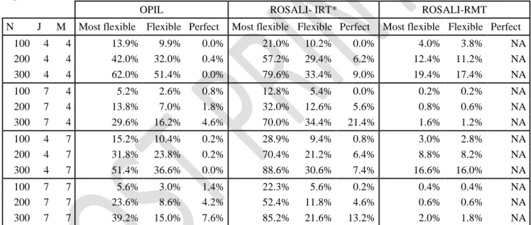
Table 3: Rates of RS detection according to simulation values of sample size (N), number of items (J) and number of answer categories (M) for datasets with RS (high values of reprioritization) simulated on 1 item.
OPIL ROSALI- IRT* ROSALI-RMT
N J M Most flexible Flexible Perfect Most flexible Flexible Perfect Most flexible Flexible Perfect 100 4 4 13.9% 9.9% 0.0% 21.0% 10.2% 0.0% 4.0% 3.8% NA 200 4 4 42.0% 32.0% 0.4% 57.2% 29.4% 6.2% 12.4% 11.2% NA 300 4 4 62.0% 51.4% 0.0% 79.6% 33.4% 9.0% 19.4% 17.4% NA 100 7 4 5.2% 2.6% 0.8% 12.8% 5.4% 0.0% 0.2% 0.2% NA 200 7 4 13.8% 7.0% 1.8% 32.0% 12.6% 5.6% 0.8% 0.6% NA 300 7 4 29.6% 16.2% 4.6% 70.0% 34.4% 21.4% 1.6% 1.2% NA 100 4 7 15.2% 10.4% 0.2% 28.9% 9.4% 0.8% 3.0% 2.8% NA 200 4 7 31.8% 23.8% 0.2% 70.4% 21.2% 6.4% 8.8% 8.2% NA 300 4 7 51.4% 36.6% 0.0% 88.6% 30.6% 7.4% 16.6% 16.0% NA 100 7 7 5.6% 3.0% 1.4% 22.3% 5.6% 0.2% 0.4% 0.4% NA 200 7 7 23.6% 8.6% 4.2% 52.4% 11.8% 4.6% 0.6% 0.6% NA 300 7 7 39.2% 15.0% 7.6% 85.2% 21.6% 13.2% 2.0% 1.8% NA
Most flexible RS detection: proportion of datasets where the method was able to identify at least the correct item among others, when RS was simulated
Flexible RS detection: proportion of datasets where any type of RS was detected and accounted for on the correct item only, when RS was simulated
Perfect RS detection: proportion of datasets where the method has detected exactly the simulated RS (correct type of RS on the correct item only), when RS was simulated NA: not applicable
* Due to high rates of false RS detection, results for ROSALI-IRT should be interpreted with caution
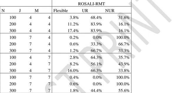
As ROSALI-RMT cannot account for RP, only UR or NUR can be detected at step 4.The proportion of each type of detected recalibration among datasets meeting flexible rate requirements (correct item where RS was simulated) at step 4 for ROSALI-RMT are
28 presented in Table 4. For datasets with J=4 items, ROSALI-RMT accounted more often for uniform recalibration whereas non-uniform recalibration was more often accounted for with 7 items.
Table 4: Type of detected recalibration among datasets meeting flexible rate requirements according to simulation values of sample size (N), number of items (J) and number of answer categories (M) for datasets with RS (high values of reprioritization) simulated on 1 item. ROSALI-RMT N J M Flexible UR NUR 100 4 4 3.8% 68.4% 31.6% 200 4 4 11.2% 83.9% 16.1% 300 4 4 17.4% 83.9% 16.1% 100 7 4 0.2% 0.0% 100.0% 200 7 4 0.6% 33.3% 66.7% 300 7 4 1.2% 66.7% 33.3% 100 4 7 2.8% 64.3% 35.7% 200 4 7 8.2% 56.1% 43.9% 300 4 7 16.0% 66.3% 33.8% 100 7 7 0.4% 0.0% 100.0% 200 7 7 0.6% 0.0% 100.0% 300 7 7 1.8% 44.4% 55.6%
Flexible RS detection: proportion of datasets where RS was detected and accounted for on the correct item only, when RS was simulated
UR (NUR): proportion of Model 4 with only uniform (non-uniform) recalibration accounted for among significant tests
Datasets with two or three items affected by RS
Globally, all methods perform similarly for simulated datasets where two or three items were affected by RS (results not shown) as compared to datasets where only one item was affected by RS. For simulated uniform and non-uniform recalibrations, ROSALI-IRT still shows the highest most flexible RS detection rates whereas ROSALI-RMT performs better than OPIL and ROSALI-IRT according to flexible and perfect detection rates.
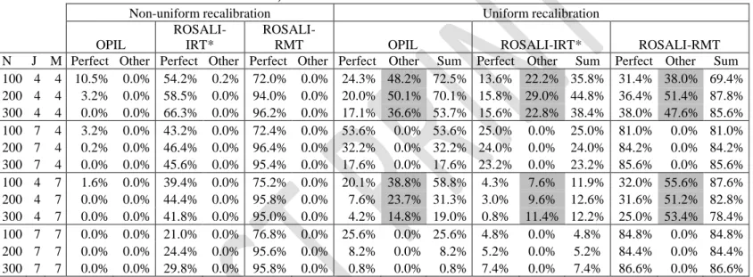
29 Largest differences between the rates of most flexible and flexible RS detection were observed for ROSALI-IRT indicating that this method very often concluded to the presence of RS on the correct items plus other items. On the opposite, large differences between rates of flexible and perfect detection were observed in case of non-uniform recalibration for OPIL when non-uniform recalibration was simulated indicating that OPIL very often concluded to NUR jointly with RP on the same item. Last, the different rates of reprioritization detection are dramatically low for OPIL and ROSALI-IRT. The cases where 2 items over 4 were affected by uniform recalibration have to be interpreted separately. In these cases, a pair of items was affected by RS and a pair of items was not affected by RS. The different rates of detection for datasets with 2 items affected by UR were surprisingly lower than for datasets with 2 items affected by NUR and lower than for datasets with 1 item affected by UR. It appeared that, in datasets with 2 items affected by UR, all methods most frequently identified the pair of items on which no RS was simulated. For example, in datasets with items 1 and 2 affected by UR, the different rates of detection computed regarding the pair of items on which no RS was simulated (items 3 and 4) were higher than the different rates of detection computed regarding the pair of items on which RS was simulated (items 1 and 2). Detection of RS on the simulated pair or on the other pair of items gives equivalent model and we had to consider the rates of perfect detection on the other pair of items as well. Rates of RS perfect detection of the simulated pair of items (items 1 and 2) and of the other pair of items (items 3 and 4) for each method are presented in Table 5. Summing perfect detection rates computed on the pair of items on which RS was simulated and perfect detection rates computed on the pair of items on which no RS was simulated (“sum”
30 column when assessing change) gave an idea of the total proportion of equivalent models. This sum gave similar rates and trends than for datasets with 1 item affected by UR. Therefore, it seems that all methods perform similarly for this particular case with a higher performance of ROSALI-RMT.
Table 5: Rates of RS perfect detection according to simulation values of sample size (N), number of items (J) and number of answer categories (M) for datasets with RS (uniform and non-uniform recalibration) simulated on 2 items.
Non-uniform recalibration Uniform recalibration OPIL
ROSALI-IRT*
ROSALI-RMT OPIL ROSALI-IRT* ROSALI-RMT
N J M Perfect Other Perfect Other Perfect Other Perfect Other Sum Perfect Other Sum Perfect Other Sum 100 4 4 10.5% 0.0% 54.2% 0.2% 72.0% 0.0% 24.3% 48.2% 72.5% 13.6% 22.2% 35.8% 31.4% 38.0% 69.4% 200 4 4 3.2% 0.0% 58.5% 0.0% 94.0% 0.0% 20.0% 50.1% 70.1% 15.8% 29.0% 44.8% 36.4% 51.4% 87.8% 300 4 4 0.0% 0.0% 66.3% 0.0% 96.2% 0.0% 17.1% 36.6% 53.7% 15.6% 22.8% 38.4% 38.0% 47.6% 85.6% 100 7 4 3.2% 0.0% 43.2% 0.0% 72.4% 0.0% 53.6% 0.0% 53.6% 25.0% 0.0% 25.0% 81.0% 0.0% 81.0% 200 7 4 0.2% 0.0% 46.4% 0.0% 96.4% 0.0% 32.2% 0.0% 32.2% 24.0% 0.0% 24.0% 84.2% 0.0% 84.2% 300 7 4 0.0% 0.0% 45.6% 0.0% 95.4% 0.0% 17.6% 0.0% 17.6% 23.2% 0.0% 23.2% 85.6% 0.0% 85.6% 100 4 7 1.6% 0.0% 39.4% 0.0% 75.2% 0.0% 20.1% 38.8% 58.8% 4.3% 7.6% 11.9% 32.0% 55.6% 87.6% 200 4 7 0.0% 0.0% 44.4% 0.0% 95.8% 0.0% 7.6% 23.7% 31.3% 3.0% 9.6% 12.6% 31.6% 51.2% 82.8% 300 4 7 0.0% 0.0% 41.8% 0.0% 95.0% 0.0% 4.2% 14.8% 19.0% 0.8% 11.4% 12.2% 25.0% 53.4% 78.4% 100 7 7 0.0% 0.0% 21.0% 0.0% 76.8% 0.0% 25.6% 0.0% 25.6% 4.8% 0.0% 4.8% 84.8% 0.0% 84.8% 200 7 7 0.0% 0.0% 24.4% 0.0% 95.6% 0.0% 8.2% 0.0% 8.2% 5.2% 0.0% 5.2% 84.4% 0.0% 84.4% 300 7 7 0.0% 0.0% 29.8% 0.0% 95.8% 0.0% 0.8% 0.0% 0.8% 7.4% 0.0% 7.4% 86.6% 0.0% 86.6%
Perfect criterion: proportion of datasets where the method has detected exactly the simulated RS (correct type of RS on the correct pair of item only), when RS was simulated
Other criterion: proportion of datasets where the method has detected the correct type of RS on the other pair of item only, when RS was simulated
Sum: sum of perfect and other criteria
Gray cells: Rates for other criterion is higher than rates for perfect criterion
* Due to high rates of false RS detection, results for ROSALI-IRT should be interpreted with caution
31 This study compared the performance of SEM (OPIL method), IRT (ROSALI-IRT
method) and RMT (ROSALI-RMT method) approaches for item-level RS detection. ROSALI-RMT performs better than OPIL and ROSALI-IRT in the light of rates of false detection, flexible detection and perfect RS detection when either UR or NUR was simulated. Consequently, if a partial-credit model fits the data, the RMT-based approach should be preferred for investigating only recalibration RS at item-level.
For all methods, a Bonferroni correction was applied at step 3 to adjust for multiple testing which is not a frequent correction in Oort’s procedure and its extensions.
However, adjusting for multiple testing seems adequate as the rates of false detection of RS based on the LRT at step 2 in datasets with no RS simulated were corrected during step 3 leading to lower rates of false detection of RS based on model 4.
Results for lower values of reprioritization ( ) and of non-uniform recalibration (shift between -0.5 and 0.5) were not shown. For all methods, rates of RS detection were much lower for these values of simulated RS parameters indicating that these values are certainly too small to be detectable by OPIL, ROSALI-IRT and ROSALI-RMT with the sample sizes that were simulated.
ROSALI-IRT method showed high most flexible RS detection rates when either UR or NUR was simulated. These high rates might be misinterpreted as an indicator of good performance. Indeed, ROSALI-IRT also presented high rates of false detection and large differences between most flexible and flexible rates of RS detection rates that tend to indicate that very often ROSALI-IRT overdetected RS by concluding to RS when no RS was simulated or identified items that were not affected by RS when RS was simulated.
32 The preliminary step used to help reaching model convergence and reduce time for
parameter estimation with the NLMIXED procedure could have been detrimental to ROSALI-IRT. In fact, the item difficulties at the first time of measurement were fixed to their estimated values at the preliminary step for all the next steps of the algorithm. This might have been unfair as the main interest in RS analysis is based on the change in item difficulties over time. Hence, ignoring the uncertainty related to the estimation of item difficulties in the preliminary step in further steps might have led to an underestimation of the variance of RS parameters and to reject the null hypothesis too often in the Wald tests of step 3. Thus, this preliminary step might be the cause of over detection of RS when no RS was simulated and to over detection of RS on items unaffected by RS when RS was simulated.
The SEM-based method OPIL showed worse performances than ROSALI-RMT. Data simulated from a different measurement theory (GPCM coming from IRT) could have penalized OPIL. The size of simulated effects are not known in SEM and might be lower than in IRT/RMT leading to RS effects more difficult to detect.
Of note, the parameters of OPIL were estimated with maximum likelihood in line with what has been frequently observed regarding the first applications of Oort’s procedure at item level (33,34). In case of ordinal data, obtaining estimations using maximum
likelihood theory is problematic as assumption of multivariate normality of the item responses is violated. In particular, chi-squares are known to be biased and so likelihood ratio tests that use the chi-square values in OPIL may lead to erroneous conclusions. Hence, the performance of OPIL could be improved by using an alternative estimation
33 method. Some studies (35,36) suggest that for ordinal data with at least five answer categories and approximately normal distribution, the ML estimation performs well. Therefore, for simulated datasets with 7 response categories, we can be quite confident that the results were not much impacted by ML estimation. However, for datasets with less than 5 response categories, OPIL performances might be improved by using
techniques to estimate SEM parameters for ordinal data recently implemented in Oort’s procedure (15,37) such as diagonally weighted least squares parameter estimation. Despite the fact that it should be encouraged to use these methods which are more suitable for ordinal data, in our study, it seemed that OPIL using maximum likelihood was pretty robust to the least favorable case (i.e. 4 response categories) because we could observe that the performance of OPIL were as good or even better with 4 as compared to 7 response categories (e.g. for false and perfect detection rates).
Apart from these technical points, large differences between flexible and perfect
detection rates were observed when NUR was simulated but not when UR was simulated. It therefore seemed that either OPIL jointly detected another type of RS along with NUR on the correct item or detected another type of RS than NUR on the correct item. By looking more thoroughly into the RS detected in datasets with one item affected by NUR, it appeared that OPIL often concluded that only one item was affected by RS (the
simulated item) but that this item was affected by NUR and RP simultaneously.
While reprioritization is easily conceptualized at dimension level (e.g. the social dimension becoming a more important indicator of quality of life after a salient health event than before), the potential different meaning and interpretation of RP at item-level
34 from a methodological or conceptual point of view has already been raised (11). To even go further, the existence of the concept of RP at item-level can be questioned. If it is easy to conceptualize that the importance of some dimensions in the definition of a
multidimensional concept can be subject to change over the disease course, it is not straightforward to expect that some items can become more important than others over time in the unidimensional context of a single dimension. The dramatically low rates of perfect detection of RP for OPIL and ROSALI-IRT are indicative of the inability of these approaches to detect RP. Although these low rates might be explained by the simulated size of RP, we can also note that due to the formulation of IRT models, a variation in discrimination power parameters (RP) might cause a variation in item difficulties
(recalibration) and inversely. Hence, trying to simulate RP in the datasets could have led to simulate also recalibration. The same problem could have occurred in SEM as a variation of factor loadings parameters (RP) might cause a variation in residual variances (NUR) and inversely. Thus, OPIL and ROSALI-IRT could have adjusted for NUR instead of RP due to the link between the RS parameters. Observed differences between the rates of flexible RS detection and of perfect detection revealed that ROSALI-IRT was able to identify the items affected by RS but not the type of simulated RS on these items. Indeed, ROSALI-IRT often concluded that items were affected by UR or NUR (change in item difficulties) when RP (change in discrimination parameters) was simulated. Similarly, OPIL often concluded that items were affected by NUR (change in residual variances) when RP (change in factor loadings) was simulated.
As expected, ROSALI-RMT showed low most flexible rates of detection for RP in particular for datasets with 7 items as RP is not operationalized in RMT. But, when RS
35 was accounted for in model 4, the item affected by RS was quite often correctly
identified.
Reconceptualization was not assessed in the simulation study. The SEM-based method OPIL is able to provide clues of reconceptualization as poor fit of measurement model in step 1 can indicate that the measurement model does not hold for both times of
measurement. On the opposite, fit indices or tests are not available for longitudinal IRT or RMT models so that ROSALI-IRT and ROSALI-RMT cannot help investigating reconceptualization. Multidimensional IRT or RMT models would be required to do so. From a conceptual point of view, item-level reconceptualization means that some items can load on one factor (the dimension of interest) at one time of measurement and load on another factor (an already existing or new dimension) at another time of measurement. Thus, level reconceptualization will probably lead to dimension-level RS. As item-level RS detection is operationalized in a unidimensional context, it seems important to also look at dimension-level RS to have a complementary insight and a comprehensive overview of RS and longitudinal change in PRO data.
ROSALI-IRT and ROSALI-RMT were described as different methods for RS detection even though it could be argued that Rasch models are embedded within IRT and that they can be shown to be mathematically equivalent (e.g. Rasch as a “special case” of IRT with all discrimination power parameters fixed to one). However, it does not mean that the models are philosophically or conceptually equivalent, RMT was originally developed to find data that fits the model while IRT models were developed to be altered in order to fit
36 the data. The rationale for distinguishing item-level RS analysis with ROSALI-RMT as compared to ROSALI-IRT was that models coming from Rasch Measurement Theory possess the specific objectivity property that can be valuable when some items are missing, in an ignorable way or not. In this study, ROSALI-RMT has shown better performances in the context of complete data. Further simulation studies taking into account the shortcomings of the present study (e.g. using more suitable SEM-based methods for ordinal data, not fixing the item difficulties at the first time of measurement to their estimated values in ROSALI-IRT, including a generating model based on the SEM framework) are now needed to confirm that ROSALI-RMT performs better than OPIL and ROSALI-IRT in particular in case of non-ignorable missing items.
RS detection relies on two strong hypotheses: all individuals of the sample are expected to experience RS the same way and RS is evaluated before and after a salient health event. We can easily understand that adaptation may not occur in the same manner for all individuals according to the various history and personality of patients even in a
homogeneous sample at baseline and that RS should be evaluated at a more individual degree. Adaptation is also not likely to occur at the same time for all individuals especially as a health event of interest can have consequences at different times in the patient’s life or the health event can be a chronic disease which can be viewed as a complex sum of events at different times over the course of illness. Investigating RS at a more individual degree and over the disease course instead than between two times of measurement (38) are important future paths of research to help understanding adaptation and improving care with specific therapies for maladaptative patients and provide
37
Funding Acknowledgments
This study was supported by the Institut National du Cancer, under reference
“INCA_6931”. Computations of ROSALI-RMT were performed thanks to the Centre de Calcul Intensif des Pays de la Loire (CCIPL) resources.
Declaration of Conflicting Interests
The Author(s) declare(s) that there is no conflict of interest
References
1. Nipp RD, Temel JS. Harnessing the Power of Patient-Reported Outcomes in
Oncology. Clin Cancer Res Off J Am Assoc Cancer Res. 2018 Apr 15;24(8):1777–9. 2. Kluetz PG, O’Connor DJ, Soltys K. Incorporating the patient experience into
regulatory decision making in the USA, Europe, and Canada. Lancet Oncol. 2018 May;19(5):e267–74.
3. Widaman KF, Ferrer E, Conger RD. Factorial Invariance within Longitudinal Structural Equation Models: Measuring the Same Construct across Time. Child Dev Perspect. 2010 Apr 1;4(1):10–8.
4. Verhagen J, Fox J-P. Longitudinal measurement in health-related surveys. A Bayesian joint growth model for multivariate ordinal responses. Stat Med. 2013 Jul 30;32(17):2988–3005.
5. Pastor DA, Beretvas SN. Longitudinal Rasch Modeling in the Context of
Psychotherapy Outcomes Assessment. Appl Psychol Meas. 2006 Mar 1;30(2):100– 20.
6. Sprangers MA, Schwartz CE. Integrating response shift into health-related quality of life research: a theoretical model. Soc Sci Med 1982. 1999 Jun;48(11):1507–15. 7. McClimans L, Bickenbach J, Westerman M, Carlson L, Wasserman D, Schwartz C.
38 8. Postulart D, Adang EM. Response shift and adaptation in chronically ill patients.
Med Decis Mak Int J Soc Med Decis Mak. 2000 Jun;20(2):186–93.
9. Oort FJ. Using structural equation modeling to detect response shifts and true change. Qual Life Res. 2005 Apr;14(3):587–98.
10. Sajobi TT, Brahmbatt R, Lix LM, Zumbo BD, Sawatzky R. Scoping review of response shift methods: current reporting practices and recommendations. Qual Life Res. 2018 May;27(5):1133–46.
11. Schwartz CE. Introduction to special section on response shift at the item level. Qual Life Res. 2016;25(6):1323–5.
12. Vanier A, Sébille V, Blanchin M, Guilleux A, Hardouin J-B. Overall performance of Oort’s procedure for response shift detection at item level: a pilot simulation study. Qual Life Res. 2015 Feb 11;24(8):1799–807.
13. Nolte S, Mierke A, Fischer HF, Rose M. On the validity of measuring change over time in routine clinical assessment: a close examination of item-level response shifts in psychosomatic inpatients. Qual Life Res. 2016;25(6):1339–47.
14. Gandhi PK, Schwartz CE, Reeve BB, DeWalt DA, Gross HE, Huang I-C. An item-level response shift study on the change of health state with the rating of asthma-specific quality of life: a report from the PROMIS® Pediatric Asthma Study. Qual Life Res. 2016 Apr 9;25(6):1349–59.
15. Verdam MGE, Oort FJ, Sprangers MAG. Using structural equation modeling to detect response shifts and true change in discrete variables: an application to the items of the SF-36. Qual Life Res. 2016;25(6):1361–83.
16. Ahmed S, Sawatzky R, Levesque J-F, Ehrmann-Feldman D, Schwartz CE. Minimal evidence of response shift in the absence of a catalyst. Qual Life Res. 2014 Nov 1;23(9):2421–30.
17. Guilleux A, Blanchin M, Vanier A, Guillemin F, Falissard B, Schwartz CE, et al. RespOnse Shift ALgorithm in Item response theory (ROSALI) for response shift detection with missing data in longitudinal patient-reported outcome studies. Qual Life Res. 2015;24(3):553–64.
18. Anota A, Bascoul-Mollevi C, Conroy T, Guillemin F, Velten M, Jolly D, et al. Item response theory and factor analysis as a mean to characterize occurrence of response shift in a longitudinal quality of life study in breast cancer patients. Health Qual Life Outcomes. 2014 Mar 8;12:32.
19. Blanchin M, Sébille V, Guilleux A, Hardouin J-B. The Guttman errors as a tool for response shift detection at subgroup and item levels. Qual Life Res Int J Qual Life Asp Treat Care Rehabil. 2016;25(6):1385–93.
39 20. Fischer GH, Molenaar IW. Rasch models: foundations, recent developments, and
applications. New York: Springer; 1995. 470 p.
21. Andrich D. Rating scales and Rasch measurement. Expert Rev Pharmacoecon Outcomes Res. 2011 Oct;11(5):571–85.
22. de Bock É, Hardouin J-B, Blanchin M, Le Neel T, Kubis G, Bonnaud-Antignac A, et al. Rasch-family models are more valuable than score-based approaches for analysing longitudinal patient-reported outcomes with missing data. Stat Methods Med Res. 2016 Oct;25(5):2067–87.
23. Hamel J-F, Hardouin J-B, Le Neel T, Kubis G, Roquelaure Y, Sébille V. Biases and Power for Groups Comparison on Subjective Health Measurements. PLoS ONE. 2012 Oct 24;7(10):e44695.
24. de Bock E, Hardouin J-B, Blanchin M, Neel TL, Kubis G, Sébille V. Assessment of score- and Rasch-based methods for group comparison of longitudinal patient-reported outcomes with intermittent missing data (informative and non-informative). Qual Life Res. 2015 Jan 1;24(1):19–29.
25. Nolte S, Elsworth GR, Sinclair AJ, Osborne RH. Tests of measurement invariance failed to support the application of the “then-test.” J Clin Epidemiol. 2009
Nov;62(11):1173–80.
26. Miller RGJ. Simultaneous Statistical Inference [Internet]. 2nd ed. New York:
Springer-Verlag; 1981 [cited 2018 May 23]. (Springer Series in Statistics). Available from: //www.springer.com/gb/book/9781461381242
27. Muraki E. A Generalized Partial Credit Model: Application of an EM Algorithm. Appl Psychol Meas. 1992 Jun 1;16(2):159–76.
28. Fischer G, Ponocny I. An extension of the partial credit model with an application to the measurement of change. Psychometrika. 1994 Jun 27;59(2):177-192–192. 29. Masters GN. A rasch model for partial credit scoring. Psychometrika. 1982
Jun;47(2):149–74.
30. Ware JE, Sherbourne CD. The MOS 36-item short-form health survey (SF-36). I. Conceptual framework and item selection. Med Care. 1992 Jun;30(6):473–83. 31. Aaronson NK, Ahmedzai S, Bergman B, Bullinger M, Cull A, Duez NJ, et al. The
European Organization for Research and Treatment of Cancer QLQ-C30: a quality-of-life instrument for use in international clinical trials in oncology. J Natl Cancer Inst. 1993;85(5):365–76.
32. Zigmond AS, Snaith RP. The Hospital Anxiety and Depression Scale. Acta Psychiatr Scand. 1983 Jun 1;67(6):361–70.
40 33. King-Kallimanis BL, Oort FJ, Nolte S, Schwartz CE, Sprangers MAG. Using
structural equation modeling to detect response shift in performance and health-related quality of life scores of multiple sclerosis patients. Qual Life Res. 2011 Jan 19;20(10):1527–40.
34. King-Kallimanis BL, Oort FJ, Lynn N, Schonfeld L. Testing the Assumption of Measurement Invariance in the SAMHSA Mental Health and Alcohol Abuse Stigma Assessment in Older Adults. Ageing Int. 2012 Dec;37(4):441–58.
35. Dolan CV. Factor analysis of variables with 2, 3, 5 and 7 response categories: A comparison of categorical variable estimators using simulated data. Br J Math Stat Psychol. 1994;47(2):309–26.
36. Muthen B, Kaplan D. A comparison of some methodologies for the factor analysis of non-normal Likert variables: A note on the size of the model. Br J Math Stat Psychol. 1992;45(1):19–30.
37. Gadermann AM, Sawatzky R, Palepu A, Hubley AM, Zumbo BD, Aubry T, et al. Minimal impact of response shift for SF-12 mental and physical health status in homeless and vulnerably housed individuals: an item-level multi-group analysis. Qual Life Res Int J Qual Life Asp Treat Care Rehabil. 2017;26(6):1463–72. 38. Barclay-Goddard R, Epstein JD, Mayo NE. Response shift: a brief overview and