HAL Id: hal-03194451
https://hal.archives-ouvertes.fr/hal-03194451
Submitted on 9 Apr 2021
HAL is a multi-disciplinary open access
archive for the deposit and dissemination of
sci-entific research documents, whether they are
pub-lished or not. The documents may come from
teaching and research institutions in France or
abroad, or from public or private research centers.
L’archive ouverte pluridisciplinaire HAL, est
destinée au dépôt et à la diffusion de documents
scientifiques de niveau recherche, publiés ou non,
émanant des établissements d’enseignement et de
recherche français ou étrangers, des laboratoires
publics ou privés.
Integration of heat transfer effects in simulation of
composite stamping
Duc Anh Hoang, Arthur Lévy, Steven Le Core
To cite this version:
Duc Anh Hoang, Arthur Lévy, Steven Le Core. Integration of heat transfer effects in simulation of
composite stamping. ESAFORM 2016:19th International ESAFORM Conference on Material
Form-ing, 2016, Nantes, France. �10.1063/1.4963574�. �hal-03194451�
Integration of Heat Transfer Effects in Simulation of
Composite Stamping
Duc Anh HOANG
1, 2, a), Arthur LEVY
1, b), Steven LE CORE
1, c)October 18, 2015
1Laboratoire de Thermocinétique de Nantes, La Chantrerie, rue Christian Pauc, BP 50609, 44306 Nantes cedex 3, France
2Institut de Recherche Technologique Jules Verne, Chemin du Chaffault, 44340, Bouguenais, France
a) duc-anh.hoang@irt-jules-verne.fr b) arthur.levy@univ-nantes.fr c) steven.lecorre@univ-nantes.fr
Abstract. A numerical method for the simulation of heat transfer occurring in thermoplastic composites thermostamping
process is proposed. A reduced thermal model, named additive decomposition, is developed. It is based on the operator splitting method under thin shell assumption. A resolution algorithm using this decomposition is proposed, and developed in MATLAB. The approach is validated by comparing solutions obtained with a full 3D resolution and the presented method. Using this method, the computational time is proved to be about over 30 times faster. Eventually, prediction of temperature field is a prerequisite for the prediction of other phenomena, such as crystallization kinetics. Finally, the proposed method is implemented in the simulation software for thermostamping process Plasfib.
INTRODUCTION
Thermoplastic composites offer new possibilities for the industry. Large structures can be processed rapidly and more cost-effectively than thermoset composites, since the latter need to undergo long curing reactions. The ability to fuse the thermoplastic resin gives new perspectives for forming processes. Thermostamping process is derived from the metal industry. Forming occurs in two steps. In a first step, a semi-finished thermoplastic flat laminate, the blank, is heated externally above the processing temperature of the matrix. In the second step, this hot blank is quickly transferred to a cold mold where it is stamped and given its final shape [1], [2]. The heating and cooling steps are therefore separated. This results in a high production rate that makes this process very attractive for the industry.
In the case of composite materials, the mechanical deformation and heat transfer occurring in the blanks may result in unexpected behavior, especially when dealing with textile composite laminates. Nonetheless, accurate modelling and prediction of the main physical phenomenon involved is a prerequisite for an efficient process optimization.
Temperature evolution rules the forming process. It controls thermal dependence of mechanical parameters and crystallization in case of semi-crystalline polymers. With this in mind, P. De Lucas et al. [3] or Cao et al. [4] proposed to take the blank temperature into account in the mechanical predictions of thermostamping process. In this process thought, and especially during the stamping step, because of the thermal shock between the cold mold and the hot blank, high through-thickness temperature gradients may arise. The models by these authors, based on rough approximations of the blank temperature, cannot accurately describe these through-thickness variations.
Furthermore, the proposed model is to be implemented in existing industrial codes. The heat transfer problem should then be solved within acceptable computational times. With this aim, the full three dimensional heat transfer problem cannot be solved using standard methods. A model reduction is necessary.
In the present study, a new numerical approach to reduce the classical 3D thermal problem is presented. A solving algorithm and numerical implementation is then proposed. The approach is validated on a plate test case whereas its limits are determined with extreme cases. Afterward, the crystallization kinetic is introduced. It is coupled with the heat transfer problem and thus requires an accurate thermal solution. Finally the proposed model integration in existing industrial codes (such as Plasfib) will be discussed.
METHODS: THERMAL SHELL REDUCED ADDITIVE MODEL
Solving a 3D thermal problem on thin shell geometry can be performed in several ways.It is natural to decompose the 3D temperature field into an out-of-plane shape function and an in-plane temperature as suggested by Saetta and Rega [5]. With this decomposition, the fine through thickness description depends on the type of shape functions chosen. Within this framework, some authors suggested to construct new 3D shell finite elements that integrate this through thickness heat transfer effects [6], [8], [9], [10]. Nonetheless, using one single shell element in the thickness highly restricts the possible through-thickness temperature profile description. Even with the higher order interpolation proposed by Surana and Abusaleh [9], sharp profiles that could arise from thermal shocks in thermostamping will never be accurately described.
On the contrary a through-thickness fine discretization can be adopted. For instance, Bognet et al. [7] wrote the above decomposition as a sum of separated modes
{𝑡𝑒𝑚𝑝𝑒𝑟𝑎𝑡𝑢𝑟𝑒3𝐷} = ∑ ({𝑠ℎ𝑎𝑝𝑒𝑖𝑛−𝑝𝑙𝑎𝑛𝑒}𝑖× {𝑡𝑒𝑚𝑝𝑒𝑟𝑎𝑡𝑢𝑟𝑒𝑜𝑢𝑡−𝑝𝑙𝑎𝑛𝑒}𝑖) 𝑖
where the shape functions, themselves, are described with a fine discretization involving hundreds of degrees of freedom. Nonetheless, in their framework, Bognet et al. considered the out-of-plane shape functions independent of the out-plane position. Using this in-plane / out-of-plane separation, a solving strategy using the proper generalized decomposition (PGD) was proposed for the elastic problem on a shell like domain. Nevertheless implementing such resolution strategies in the environments of existing codes might be challenging. In particular, dealing with space varying boundary conditions and material non-linearity requires complicated developments.
In this paper, we propose a method to reduce the heat transfer problem in the thin shell domain. By using the general decomposition of the temperature field and a thin shell assumption, we obtain the reduced boundary value problem.
3D Heat equation
Concerning the heat conduction problem in the blank, in the present work, it is assumed that the through thickness direction z is a principal direction of the thermal conductivity. So, the heat equation can be written
𝜌. 𝐶𝑝. 𝜕𝑇 𝜕𝑡 = ∇𝑠∙ (𝑲𝒔∙ ∇𝑠𝑇) + 𝜕 𝜕𝑧(𝐾𝑧 𝜕𝑇 𝜕𝑧) (1)
where 𝑲𝒔 is the in–plane thermal conductivity tensor, 𝐾𝑧 is the through-thickness thermal conductivity. T is the
temperature field and ∇𝑠∙ the in-plane surface derivative operator. 𝜌 is the density of the composite material and 𝐶𝑝
is its specific heat.
Reduced boundary value problem
The first step in the proposed model reduction is to seek the solution T of the 3D heat equation (eq(1)) as a sum of a through thickness average field and a fluctuation field. In this equation, (x,y,z) denote a local curvilinear parameterization of the geometry, where z is the coordinate along the normal to the shell
𝑇(𝑥, 𝑦, 𝑧, 𝑡) = 〈𝑇〉𝑧(𝑥, 𝑦, 𝑡) + 𝑇̃(𝑥, 𝑦, 𝑧, 𝑡) (2)
where the operator 〈∗〉𝑧 is the through thickness average. It is obvious that using this additive decomposition, the
average field 〈𝑇〉𝑧 does not depend on the z-coordinate whereas the fluctuation field 𝑇̃ has a zero average (〈𝑇̃〉𝑧=
0).
The average field heat equation, which rules the in-plane field temperature evolution, is obtained by applying the average operator 〈∗〉𝑧 on both hands of the heat equation (1) and neglecting the possible variations of 𝑲𝒔 along the
𝜌. 𝐶𝑝. 𝜕〈𝑇〉𝑧 𝜕𝑡 = ∇𝑠∙ (𝑲𝒔∙ ∇𝑠〈𝑇〉𝑧) + Φ𝑠𝑢𝑝− Φ𝑖𝑛𝑓 ℎ (3) where: Φ𝑠𝑢𝑝 = 𝐾𝑧 𝜕𝑇̃ 𝜕𝑧 (𝑧 = ℎ/2) Φ𝑖𝑛𝑓= 𝐾𝑧 𝜕𝑇̃ 𝜕𝑧 (𝑧 = −ℎ/2) (4)
with ℎ being the thickness of composite blank.
The fluctuating heat equation is obtained by subtracting the equation above from equation (1) and by considering the thin plate assumption (‖𝐾𝑠‖
|𝐾𝑧|(
ℎ 𝐿)
2
≪ 1) where 𝐿 the blank length. 𝜌. 𝐶𝑝. 𝜕𝑇̃ 𝜕𝑡 = 𝜕 𝜕𝑧(𝐾𝑧 𝜕𝑇̃ 𝜕𝑧) − Φ𝑠𝑢𝑝− Φ𝑖𝑛𝑓 ℎ (5)
Summing equation (3) and (5), and adding the term 𝜕
𝜕𝑧(𝐾𝑧 𝜕〈𝑇〉𝑧 𝜕𝑧 ) = 0, gives 𝜌. 𝐶𝑝. 𝜕𝑇 𝜕𝑡 = ∇𝑠∙ (𝑲𝒔∙ ∇𝑠〈𝑇〉𝑧) + 𝜕 𝜕𝑧(𝐾𝑧 𝜕𝑇 𝜕𝑧) (6)
In the bulk equation (6), the first spatial differential operator that appears on the right hand side acts on the average part of the temperature field 〈𝑇〉𝑧 only. Thus, this reduced boundary value problem is not trivial to solve. In
the next section, a numerical method is proposed to solve this original model. It will also confirm its well posedness.
Numerical implementation
Equation (6) is a time evolution equation. With the aim of solving it numerically, a standard incremental iterative time integration scheme is considered. At the given time step 𝑡𝑛, the solution 𝑇𝑛 is supposed to be known. Then, the
solution 𝑇𝑛+1 is searched at next time step 𝑡𝑛+1= 𝑡𝑛+ 𝑑𝑡. Applying the operator splitting strategy [11] and the
additive decomposition (2), the algorithm consists in performing two steps respectively:
Step 1: solve the 1D boundary value problem called (𝑃𝑧) over one full time step dt. It gives the intermediate
result 𝑇𝑛+1/2(𝑥, 𝑦, 𝑧) at the end of the time step 𝑡𝑛+ 𝑑𝑡
{ 𝜌. 𝐶𝑝. 𝜕𝑇 𝜕𝑡 = 𝜕 𝜕𝑧(𝐾𝑧 𝜕𝑇 𝜕𝑧) 𝐾𝑧 𝜕𝑇 𝜕𝑧= ℎ𝑠𝑢𝑝(𝑇 − 𝑇𝑖𝑚𝑝 𝑠𝑢𝑝 ) on Γ𝑠𝑢𝑝 𝐾𝑧 𝜕𝑇 𝜕𝑧= ℎ𝑖𝑛𝑓(𝑇 − 𝑇𝑖𝑚𝑝 𝑖𝑛𝑓 ) on Γ𝑖𝑛𝑓 𝑇 = 𝑇𝑛 at 𝑡 = 𝑡𝑛 (7)
FIGURE 1. Resolution strategy. At each time step, the solution is obtained with two successive steps: solving a set of 𝑁𝑚
where ℎ𝑠𝑢𝑝 and ℎ𝑖𝑛𝑓 are the exchange coefficients of the upper and lower surfaces. Step 2: solve the 2D boundary value problem over one full time step dt.
{ 𝜌. 𝐶𝑝. 𝜕〈𝑇〉𝑧 𝜕𝑡 = ∇𝑠∙ (𝑲𝒔∙ ∇𝑠〈𝑇〉𝑧) ∇𝑠〈𝑇〉𝑧. 𝑛 = 0 on Γ𝑙𝑎𝑡 〈𝑇〉𝑧= 〈𝑇𝑛+1/2〉𝑧 (8)
where the initial condition 𝑇𝑛+1/2 is the value of the field computed in step 1. The final solution of this second step
is identified to 〈𝑇𝑛+1〉𝑧. Both (𝑃𝑧) et (𝑃𝑠) can be solved with classical numerical method (in this work, a finite
element method is used). Then the solution 𝑇𝑛+1 is obtained as:
𝑇𝑛+1(𝑥, 𝑦, 𝑧) = 〈𝑇𝑛+1〉𝑧(𝑥, 𝑦) + 𝑇𝑛+1/2(𝑥, 𝑦, 𝑧) − 〈𝑇𝑛+1/2〉𝑧(𝑥, 𝑦) (9)
RESULTS AND DISCUSSION
Validation
In this section, the reference temperature fields 𝑇𝑟𝑒𝑓 are first obtained by solving an initial three dimensional
problem using a commercial software (COMSOL). It is then compared to the temperature fields 𝑇𝑠𝑒𝑝 obtained by
following the additive decomposition strategy presented above. In this test case, a square flat plate of PA66/glass fibers of dimensions 0.1 × 0.1 m2 and thickness h=5mm is considered. The material properties are adapted from
[12]. The in-plane conductivity 𝑲𝒔 is considered isotropic obtained from the supplier. All the material properties are
supposed constant and are listed in Table 1.
In order to add in-plane variability to the problem, the exchange coefficients ℎ𝑠𝑢𝑝 and ℎ𝑖𝑛𝑓 depend on space
with the characteristic Gaussian function:
𝜒(𝑥, 𝑦) = exp (−500 (𝑥
2+ 𝑦2
𝐿2 ) (10)
The boundary and initial conditions are given in Table 2.
TABLE 1. Material properties used in the test case.
Density 1870 𝑘𝑔. 𝑚−3
Specific heat 𝐶𝑝 990 𝐽. 𝐾−1. 𝑘𝑔−1
In-plane conductivity 𝐾𝑝𝑝, 𝐾𝑞𝑞 0.44 𝑊. 𝑚−1. 𝐾−1
Out-plane conductivity 𝐾𝑧 0.53 𝑊. 𝑚−1. 𝐾−1 TABLE 2. Initial and boundary conditions used in the test case.
Initial temperature 𝑇𝑖𝑛𝑖𝑡 20 °𝐶
Exchange coefficients ℎ𝑠𝑢𝑝, ℎ𝑖𝑛𝑓 105𝑊. 𝑚−2. 𝐾−1× 𝜒(𝑥, 𝑦)
Imposed temperature 𝑇𝑖𝑚𝑝𝑠𝑢𝑝 300 °𝐶 𝑇𝑖𝑚𝑝𝑖𝑛𝑓 250 °𝐶
Mesh: A 3D regular mesh made of 108000 hexahedrons is obtained by extruding a regular in-plane 2D mesh
that consists of 60 × 60 quadrangular elements. There are thus 30 elements in the thickness, and in terms of nodes, 𝑁𝑚= 3721 (in-plane nodes) and 𝑁𝑧= 31 (through thickness nodes).
The mesh used in the presented separated method consists of the same 31 nodes through thickness for the 𝑃𝑧
problems and a triangular regular mesh with the same 10201 nodes for the 𝑃𝑚 problem.
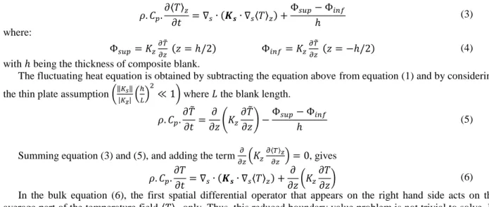
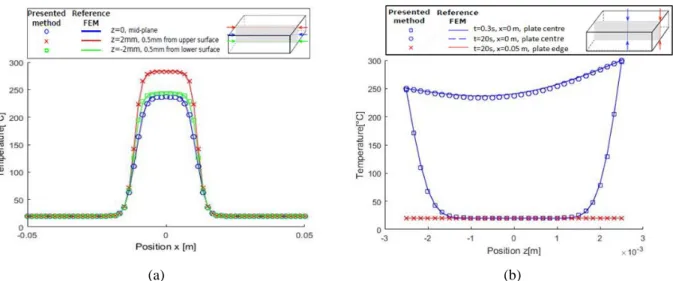
The interpolations used in every finite element methods (3D in COMSOL, 2D in 𝑃𝑚 and 1D in 𝑃𝑧) are linear P1. Comparison: Figure 2a shows the in-plane temperature profiles at three different heights at final time 𝑡 = 20 𝑠. Figure 2b represents the through thickness temperature profiles in the center and on the edge of the plate at time 𝑡 = 0.3 𝑠 and 𝑡 = 20 𝑠. The figures show a good superposition of the reference field obtained with the finite element simulation and the one obtained with the presented method. The maximal error, which is located at the middle point, is about 4°C (2% of the temperature evolution).
(a) (b)
FIGURE 2. (a) Temperature profile at y = 0 versus x for three different heights z in the plate at final time t = 20s. (b)
Temperature profile at y = 0 versus z for two different positions in-plane x and two different instants t=0.3s and t=20s.
Speed up
The reference FE simulation was computed on a desktop computer. In COMSOL, the solving time for one time step is about 5.4 s. The separated form solution was computed on the same computer, with about 0.16s per time step. This represented a speed up of over 30 times. The solving of several 1D problems and a single 2D problem is less expensive than 3D problem. Moreover, the 𝑃𝑧 problems are solved in a sequential manner in this test case. Because
they are independent, a parallel resolution could be easily implemented and would result in increased speed-up.
Crystallization-kinetic
Starting from temperature solution obtained with the additive decomposition model presented in the previous section, the crystallization problem can be solved. In the process of thermo-stamping, the phenomenon of crystallization occurs during the cooling phase (consolidation phase). In this section, we are interested in predicting this phenomenon at the macroscopic scale. This physical transformation is represented by the crystallization degree 𝛼. 𝛼 is defined as the advancement of the crystallization. 𝛼 ranges from 0 (amorphous) to 1 (maximum of crystallization).
The thermal crystallization of semi-crystalline polymers can classically be modeled by Nakamura law [13]:
𝜕𝛼
𝜕𝑡 = 𝛼̇ = 𝑛𝐾𝑛(𝑇)𝑔(𝛼) (11) Where: 𝐾𝑛(𝑇) is the kinetic function which rules the temperature activation of the phenomenon
𝑛 is the Nakamura’s exponent 𝑔(𝛼) is the Nakamura’s function
𝑔(𝛼) = (1 − 𝛼)(−𝑙𝑛(1 − 𝛼))
𝑛−1
𝑛 (12)
Resolution method: The crystallization-kinetics is a first-order ordinary differential equation and needs to be solved at every material point. A time integration scheme could be used. The coupling between heat transfer and crystallization makes the problem nonlinear. A Newton-Raphson method was therefore adopted here.
Implementation of presented model in existing code
For the numerical simulation of the composite forming process, existing industrial codes can predict the mechanical behavior and the geometry of the prepreg and textile. We may cite PAMFORM [16], Aniform [14], Plasfib [15] etc… However these codes lack the effect of temperature. In future work, we wish to simulate the influence of thermo-kinetics behavior on the material by implementing the presented model in Plasfib code. For each time step, an exchange of data between Plasfib and the presented model is performed. Specifically, the thermal
module retrieves the coordinates of the nodes and the list of nodes in contact plate/tools for updating the boundary conditions of the thermal problem 𝑃𝑧 (7). The finite elements used in Plasfib are 2D triangular elements. The
problem 𝑃𝑠 (8) can be solved using the same framework. For each in-plane position, we can easily solve a (1D)
problem 𝑃𝑧. Inversely, Plasfib code will retrieve the temperature value for each node from the thermal model. Using this temperature field effect, the material properties will be updated.
REFERENCES
1. M. Hou, “Stamp forming of continuous glass fibre reinforced polypropylene,” Compos. Part A Appl. Sci.
Manuf., vol. 28, no. 8, pp. 695–702, 1997.
2. Hugues Lessard, “Evaluation expérimentale du proceed de thermoformage-estampage d’un composite PEEK/Carbone constitué de plis unidirectionels,” PhD thesis, Université du Québec à Trois Rivières, 2014. 3. P. de Luca, P. Lefébure, and a. K. Pickett, “Numerical and experimental investigation of some press forming
parameters of two fibre reinforced thermoplastics: APC2-AS4 and PEI-CETEX,” Compos. Part A Appl. Sci.
Manuf., vol. 29, no. 1–2, pp. 101–110, 1998.
4. J. Cao, P. Xue, X. Peng, and N. Krishnan, “An approach in modeling the temperature effect in thermo-stamping of woven composites,” Compos. Struct., vol. 61, no. 4, pp. 413–420, 2003.
5. Eduardo Saetta and Giuseppe Rega, “Unified 2D continuous and reduced order modeling of thermomechanically coupled laminated plate for nonlinear vibrations,” Meccanica, vol. 49, no. 8, pp. 1723– 1749, 2014.
6. G. Bergman and M. Oldenburg, “A finite element model for thermomechanical analysis of sheet metal forming,” Int. J. Numer. …, vol. 1186, no. October 2002, pp. 1167–1186, 2004.
7. B. Bognet, F. Bordeu, F. Chinesta, a. Leygue, and a. Poitou, “Advanced simulation of models defined in plate geometries: 3D solutions with 2D computational complexity,” Comput. Methods Appl. Mech. Eng., vol. 201– 204, pp. 1–12, 2012.
8. K. S. Surana and R. K. Phillips, “Three dimensional curved shell finite elements for heat conduction,” Comput.
Struct., vol. 25, no. 5, pp. 775–785, 1987.
9. K. S. Surana and G. Abusaleh, “Curved shell elements for heat conduction with p-approximation in the shell thickness direction,” Comput. Struct., vol. 34, no. 6, pp. 861–880, 1990.
10. Raimund Rolfes, Jan Tebmer, Institut Strukturmechanik, and V Dlr, “2D Finite Element Formulation for 3D Temperature Analysis of Layered Hybrid Structures,” In NAFEMS Seminar: Numerical Simulation of Heat Transfer, Wiesbaden, Germany,2001.
11. Jim Douglas, “On the numerical integration of 𝜕
2𝑢
𝜕𝑥2+ 𝜕2𝑢 𝜕𝑦2=
𝜕𝑢
𝜕𝑡 by implicit Methods,” Journal of the society for
industrial and applied mathematics, vol. 3, no.1, pp. 42-65, 1955.
12. J. Faraj, B. Pignon, J.-L. Bailleul, N. Boyard, D. Delaunay, and G. Orange, “Heat transfer and crystallization modeling during compression molding of thermoplastic composite parts,” Key Eng. Mater., vol. 651–653, no. November, pp. 1507–1512, 2015.
13. K. Nakamura, T. Watanabe, and K. Katayama, “Some aspects of nonisothermal crystallization of polymers. I. Relationship between crystallization temperature, crystallinity, and cooling conditions,” J. Appl. Polym. Sci., vol. 16, no. 5, pp. 1077–1091, 1972.
14. S. P. Haanappel and R. Akkerman, “FORMING PREDICTIONS OF UD REINFORCED THERMOPLASTIC LAMINATES,” no. June, pp. 1–10, 2010.
15. P. Wang, X. Legrand, and P. Boisse, “Experimental and numerical analyses of manufacturing process of a composite square box part : Comparison between textile reinforcement forming and surface 3D weaving,” vol. 78, pp. 26–34, 2015.
16. P. de Luca, P. Lefébure, and a. K. Pickett, “Numerical and experimental investigation of some press forming parameters of two fibre reinforced thermoplastics: APC2-AS4 and PEI-CETEX,” Compos. Part A Appl. Sci.