Inclusion-exclusion principle for belief functions

O

pen

A

rchive

T

OULOUSE

A

rchive

O

uverte (

OATAO

)

OATAO is an open access repository that collects the work of Toulouse researchers and

makes it freely available over the web where possible.

This is an author-deposited version published in :

http://oatao.univ-toulouse.fr/

Eprints ID : 13208

To link to this article :

DOI:10.1016/j.ijar.2014.04.018

URL :

http://dx.doi.org/10.1016/j.ijar.2014.04.018

To cite this version :

Aguirre, Felipe and Destercke, Sébastien and Dubois, Didier

and Sallak, Mohamed and Jacob, Christelle Inclusion-exclusion principle for belief

functions. (2014) International Journal of Approximate Reasoning, vol. 55 (n° 8).

pp. 1708-1727. ISSN 0888-613X

Any correspondance concerning this service should be sent to the repository

administrator:

staff-oatao@listes-diff.inp-toulouse.fr

Inclusion–exclusion principle for belief functions

F. Aguirre

a

, S. Destercke

b

, D. Dubois

c

, M. Sallak

b

, C. Jacob

c

,

d

a_{Phimeca, 18/20 boulevard de Reuilly, F-75012 Paris, France}

b_{CNRS/UTC, UMR Heudiasyc, Centre de recherche de Royallieu, 60205 Compiègne, France} c_{IRIT CNRS, Université Paul Sabatier de Toulouse, France}

d_{ISAE, Toulouse, France}

a b s t r a c t

Keywords: Belief function Inclusion–exclusion principle Reliability analysis Boolean formula Independence

The inclusion–exclusion principle is a well-known property in probability theory, and is instrumental in some computational problems such as the evaluation of system reliability or the calculation of the probability of a Boolean formula in diagnosis. However, in the setting of uncertainty theories more general than probability theory, this principle no longer holds in general. It is therefore useful to know for which families of events it continues to hold. This paper investigates this question in the setting of belief functions. After exhibiting original sufficient and necessary conditions for the principle to hold, we illustrate its use on the uncertainty analysis of Boolean and non-Boolean systems in reliability.

1. Introduction

Probability theory is the most well-known approach to model uncertainty. However, even when the existence of a sin-gle probability measure is assumed, it often happens that its distribution is only partially known. This is particularly the case in the presence of severe uncertainty (few samples, imprecise or unreliable data, etc.) or when subjective beliefs are elicited (e.g., from experts). Some authors use a selection principle that brings us back to a precise distribution (e.g.,

maxi-mum entropy[23]), but other ones[28,26,16]have argued that in some situations involving imprecision or incompleteness,

uncertainty cannot be modelled faithfully by a single probability measure. The same authors have advocated the need for

frameworks accommodating imprecision, their efforts resulting in different frameworks such as possibility theory[16], belief

functions[26], imprecise probabilities[28], info-gap theory[4], etc. that are formally connected[29,17]. Regardless of

inter-pretive issues, the formal setting of belief functions offers a good compromise between expressiveness and calculability, as it is more general than probability theory, yet in many cases remains more tractable than imprecise probability approaches. Nevertheless using belief functions is often more computationally demanding than using probabilities. Indeed, its higher level of generality prevents the use of some properties, valid in probability theory, that help simplify calculations. This is the case, for instance, for the well-known and useful inclusion–exclusion principle (also known as Sylvester–Poincaré equality).

Given a space

X

, a probability measure P over this space and any collection

A

_n

= {

A1

, . . . ,

An|Ai

⊆ X }

of measurable

P

Ã

n

[

i=1 Ai

!

=

X

I⊆An

(−

1

)

|I |+1P

µ

\

A∈I A

¶

(1)

where

|I |

is the cardinality of

I

. This equality allows us to easily compute the probability of

Sn

_i=1Ai, when the events

Ai are stochastically independent, or when their intersections are disjoint. This principle has been applied to numerous

problems, including the evaluation of the reliability of complex systems. It does not hold for belief functions, and only an

inequality remains. However, it is useful to investigate whether or not an equality can be restored for specific families

A

_n

of events, in particular the ones encountered in applications to diagnosis and reliability. The main contribution of this paper is to give a positive answer to this question and to provide conditions characterising the families of events for which the inclusion–exclusion principle still holds in the belief function setting.

This paper is organised as follows. First, Section 2 provides sufficient and necessary conditions under which the

inclusion–exclusion principle holds for belief functions in general spaces; it is explained why the question may be more

difficult for the conjugate plausibility functions. Section3then studies how the results apply to the practically interesting

case where events Ai and focal elements are Cartesian products in a multidimensional space. Section 4 investigates the

particular case of binary spaces, and considers the calculation of the degree of belief and plausibility of a Boolean formula

expressed in Disjunctive Normal Form (DNF). Section5 then shows that specific events described by means of monotone

functions over a Cartesian product of totally ordered discrete spaces meet the conditions for the inclusion–exclusion

princi-ple to hold. Section6is devoted to illustrative applications of the preceding results to the field of reliability analysis (both

for the binary and non-binary cases), in which the use of belief functions is natural and the need for efficient computation

schemes is an important issue. Finally, Section7compares our results with those obtained when assuming stochastic

inde-pendence between ill-known probabilities, displaying those cases for which these results coincide and those for which they disagree.

This work extends the results concerning the computation of uncertainty bounds within the belief function framework

previously presented in [22,1]. In particular, we provide full proofs as well as additional examples. We also discuss the

application of the inclusion/exclusion principle to plausibilities, as well as a comparison of our approach with other types

of independence notions proposed for imprecise probabilities (two issues not tackled in[22,1]).

2. General additivity conditions for belief functions

After introducing some notations and the basics of belief functions (Section 2.1), we explore in Section 2.2 general

conditions for families of subsets for which the inclusion–exclusion principle holds for belief functions. We then look more closely at the specific case where the focal elements of belief functions are Cartesian products of subsets. Readers not

interested in technical details and familiar with belief functions may directly move to Section3.

2.1. Setting

A mass distribution [26] defined on a (finite) space

X

is a mapping m

:

2X

_{→ [}

₀

,

1

]

from the power set of

X

to

the unit interval such that m

(∅) =

0 and

P

_E⊆Xm

(

E

) =

1. A set E that receives a strictly positive mass is called a focal

element, and the set of focal elements of m is denoted by

F

_m. The mass function m can be seen as a probability distribution over sets, in this sense it captures both probabilities and sets: any probability p can be modelled by a mass m such that

m

({

x

}) =

p

(

x

)

and any set E can be modelled by the mass m

(

E

) =

1. In the setting of belief functions, a focal element is

understood as a piece of incomplete information of the form x

∈

E for some parameter x of interest. Then m

(

E

)

can be

understood as the probability that all that is known about x is that x

∈

E; in other words, m

(

E

)

is a probability mass that

should be divided over elements of E but is not, due to a lack of information.

From the mapping m are usually defined two set-functions, the belief and the plausibility functions, respectively defined

for any A

⊆ X

as Bel

(

A

) =

X

E⊆A m

(

E

),

(2) Pl

(

A

) =

X

E∩A6=∅ m

(

E

) =

1

−

Bel

¡

Ac

¢

,

(3)

with Ac the complement of A. They satisfy Bel

(

A

) ≤

Pl

(

A

)

. The belief function, which sums all masses of subsets that

im-ply A, measures how much event A is certain, while the plausibility function, which sums all masses of subsets consistent

with A, measures how much the event A is possible. Within the so-called theory of evidence [26], belief and plausibility

functions are interpreted as confidence degrees about the event A, and are not necessarily related to probabilities. However, the mass distribution m can also be interpreted as the random set corresponding to an imprecisely observed random

vari-able [12], and the measures Bel and Pl can be interpreted as describing a set of probabilities, that is, we can associate to

them a set

P (

Bel

)

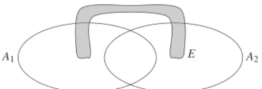
such that

Fig. 1. Focal element E of non-additive belief function for{A1,A2}.

is the set of all probabilities bounded by Bel and Pl. The belief function can then be computed as a lower probability

Bel

(

A

) =

infP∈P(Bel)P

(

A

)

and the plausibility function likewise as an upper probability. Note that, since Bel and Pl are

conjugate (Bel

(

A

) =

1

−

Pl

(

Ac

₎

_{), we can restrict our attention to one of them.}

Consider now a collection of events

A

_n

= {

A1

, . . . ,

An|Ai

⊆ X }

of subsets of

X

and a mass distribution m from which

a belief function Bel can be computed. For any collection

A

_nthe inequality[26]

Bel

Ã

n

[

i=1 Ai

!

≥

X

I⊆An

(−

1

)

|I |+1Bel

µ

\

A∈I A

´

(4)

is valid. This property is called order-n supermodularity, and belief functions are super-modular for any n

>

0. While the

inclusion–exclusion property (1)of probabilities is a mere consequence of the additivity axiom (for n

=

2),

supermodu-larity of order n does not imply supermodusupermodu-larity of order n

+

1; and the supermodularity property valid at any order is

characteristic of belief functions.

If Eq.(4)is an equality for some family

A

_n, we say that the belief function is additive for this collection, or

A

_n-additive,

for short. Eq.(4)is to be compared to Eq.(1). Note that in the following we can assume without loss of generality that for

any i

,

j, Ai

*

Aj, i.e., there is no pairwise inclusion relation between the sets of

A

n (otherwise Ai can be suppressed from

Eq.(4)). Then the family

A

_nis said to be proper.

2.2. General necessary and sufficient conditions

In the case of two events A1 and A2, neither of which is included in the other, the basic condition for the inclusion–

exclusion law to hold is that focal elements in A1

∪

A2should only lie (be included) in A1 or A2. Indeed, otherwise, if there

exists an event E

⊆

A1

∪

A2 with E

*

A1, E

*

A2and m

(

E

) >

0, then

Bel

(

A1

∪

A2

) ≥

m

(

E

) +

Bel

(

A1

) +

Bel

(

A2

) −

Bel

(

A1

∩

A2

)

>

Bel

(

A1

) +

Bel

(

A2

) −

Bel

(

A1

∩

A2

).

This means that, in order to ensure

{

A1

,

A2

}

-additivity, one must check that

F

_m

_∩

₂A1∪A2

₌

F

_m

_∩

¡

₂A1

_∪

₂A2

¢

₍₅₎

where 2C _{denotes the set of subsets of C . So, one must check that for all events E}

_{∈ Fm}

_{such that E}

_{⊆ (}

_A

1

∪

A2

)

, either

E

⊆

A1 or E

⊆

A2, or equivalently

Lemma 1. Abelief function is additive for

{

A1

,

A2

}

if and only if for all events E

⊆

A1

∪

A2 such that

(

A1

\

A2

) ∩

E

6= ∅

and

(

A2

\

A1

) ∩

E

6= ∅

then m

(

E

) =

0.

Proof. Immediate, as E overlaps A1 and A2 without being included in one of them if and only if

(

A1

\

A2

) ∩

E

6= ∅

and

(

A2

\

A1

) ∩

E

6= ∅

.

✷

Note that if

{

A1

,

A2

}

is not proper, the belief function is trivially additive for it.Fig. 1provides an illustration of a focal

element that makes a belief function non-additive for events A1 and A2. This result can be extended to the case where

A

_n

= {

A1

, . . . ,

An|Ai

⊆ X }

in a quite straightforward way:

Proposition 1.

F

_m

∩

2A1∪...∪An

_{= Fm}

_{∩ (}

₂A1

_{∪ . . . ∪}

₂An

_{) ⇔ ∀}

_E

_{⊆ (}

_A1

_{∪ . . . ∪}

_{An), if E}

_{∈ Fm}

_then

∄

_Ai,Ajwith

₍

_Ai

_\

_{Aj) ∩E}

_{6= ∅}

and

(

Aj

\

Ai) ∩E

6= ∅

.

Proof.

F

_m

∩

2A1∪...∪An

_{= Fm}

_{∩ (}

₂A1

_{∪ . . . ∪}

₂An

₎

if and only if

∄

E

∈ Fm

∩ (

2A1∪...∪An

_{\ (}

₂A1

_{∪ . . . ∪}

₂An

₎₎

if and only if

∄

E

⊆ (

A1

∪ . . . ∪

An),E

∈ Fm

such that

∀

i

=

1

, . . . ,

n

,

E

*

Ai

if and only if

∄

i

6=

j

,

E

∈ Fm,

E

*

Ai,E

*

Aj,E

∩

Ai

6= ∅,

E

∩

Aj

6= ∅

if and only if

∄

i

6=

j

,

E

∈ Fm

, with

(

Ai

\

Aj) ∩E

6= ∅

and

(

Aj

\

Ai) ∩E

6= ∅

.

✷

Fig. 2. Focal element E of non-additive plausibility function for{A1,A2}. Theorem 2. The equality

Bel

Ã

n

[

i=1 Ai

!

=

X

I⊆An

(−

1

)

|I |+1Bel

µ

\

A∈I A

¶

(6)

holds if and only if for all E

⊆ (

A1

∪ . . . ∪

An), if m

(

E

) >

0 then there is no pair Ai,Ajwith

(

Ai

\

Aj) ∩E

6= ∅

and

(

Aj

\

Ai) ∩E

6= ∅

.

Theorem 2 shows that going from

A

₂-additivity to

A

_n-additivity is straightforward, as ensuring

A

_n-additivity comes

down to checking the conditions of

A

₂-additivity for every pair of subsets in

A

_n. This feature makes the verification of the

property rather inexpensive. Finally, note that if the family

A

_n is not proper, it means Aj

⊆

Ai for some i

6=

j and it is then

impossible that

∃

E

, (

Ai

\

Aj) ∩E

6= ∅

and

(

Aj

\

Ai) ∩E

6= ∅

. So, we can dispense with checking the condition for those pairs

of sets.

2.3. Inclusion–exclusion for plausibilities

Note that by duality one also can write a form of inclusion–exclusion property for plausibility functions:

Pl

Ã

_n

\

i=1 Bi

!

=

X

I⊆Bn

(−

1

)

|I |+1Pl

µ

[

B∈I B

¶

(7)

for a family of sets

B

_n

= {

Ac_i

:

Ai

∈ An}

where

A

n satisfies the condition ofProposition 1. Although Eq.(7)provides us with

a kind of inclusion–exclusion property for plausibilities, it does not provide insight about the conditions under which the equality Pl

Ã

_n

[

i=1 Ai

!

=

X

I_⊆An

(−

1

)

|I |+1Pl

µ

\

A∈I A

¶

(8)

holds. In this section, we will investigate this issue, concluding that the case of plausibility functions is harder to deal with, and less practically interesting than the case of belief functions.

Let us first deal with two events A1 and A2. In this case, any focal element E overlapping A1

∪

A2 should not overlap

A1 and A2 without overlapping A1

∩

A2, otherwise let

E

be the non-empty set of focal elements that overlap A1 and A2

without overlapping A1

∩

A2. It is then clear that Pl is strictly submodular, i.e.:

Pl

(

A1

∪

A2

) +

X

E∈E

m

(

E

) =

Pl

(

A1

) +

Pl

(

A2

) −

Pl

(

A1

∩

A2

)

and additivity fails. This leads us to the following condition for a plausibility function to be

A

₂-additive.

Lemma 2. A plausibility function is

A

₂-additive for

A

₂

_{= {}

A1

,

A2

}

if and only if

∀

E

∩ (

A1

∪

A2

) 6= ∅

such that E

∩ (

A1

\

A2

) 6= ∅

,

E

∩ (

A2

\

A1

) 6= ∅

and E

∩ (

A1

∩

A2

) = ∅

, then m

(

E

) =

0.

It should be noted that this condition is similar to, but quite different from the one inLemma 1, as any set overlapping

A1

∩

A2 but not included in A1

∩

A2 can receive a positive mass without leading to a violation of

A

2-additivity for the

associated plausibility function. This is not the case for belief functions: for instance, the focal element of Fig. 1is not in

contradiction withLemma 2(plausibility could still be

A

₂-additive). Fig. 2pictures a focal element that would make the

plausibility not

A

₂-additive.

Nevertheless, the condition for

A

₂-additivity inLemma 2can be equivalently expressed as follows

F

_m

∩

2(Ac1∪Ac2)

=

F

_m

∩

¡

2Ac1

∪

₂Ac2

¢

_,

which can be deduced from Eq. (5), using the fact that for two subsets A1

,

A2, the

A

2-additivity of a plausibility function

is equivalent to the

A

₂-additivity of the dual belief function for Ac₁

,

A₂c (clearly, Pl

(

A1

∪

A2

) =

Pl

(

A1

) +

Pl

(

A2

) −

Pl

(

A1

∩

A2

)

is the same equation as Bel

(

Ac₁

∪

Ac₂

) =

Bel

(

Ac₁

) +

Bel

(

Ac₂

) −

Bel

(

Ac₁

∩

Ac₂

)

).

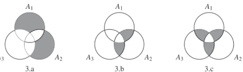
Fig. 3. PlausibilityA₃-additivity illustration.

However, the situation for plausibility functions is more involved than the one for belief functions, andLemma 2cannot

be straightforwardly extended to the case of n events, as the

A

₃-additivity of a plausibility function for A1

,

A2

,

A3:

Pl

(

A1

∪

A2

∪

A3

) =

X

Ai Pl

(

Ai

)

|

{z

}

term 1

−

X

Ai,Aj Pl

(

Ai

∩

Aj

)

|

{z

}

term 2

+

Pl

(

A1

∩

A2

∩

A3

)

|

{z

}

term 3 (9)

is no longer equivalent to

A

₃-additivity for the conjugate belief function for Ac₁

,

Ac₂

,

Ac₃. For one, the two equations are no

longer the same. Moreover, the condition

F

_m

∩

2(Ac1∪Ac2∪Ac3)

=

F

_m

∩

¡

2Ac1

∪

₂Ac2

∪

₂Ac3

¢

no longer ensures the

A

₃-additivity of the plausibility function. For instance if E

= (

A1

\ (

A2

∪

A3

)) ∪ (

A2

\ (

A1

∪

A3

))

,

a subset of Ac

3pictured inFig. 3.a, is focal, the mass of this element is counted once in the left-hand side of Eq.(9), twice in

term 1 and zero times in terms 2 and 3 of the right-hand side, so

A

₃-additivity fails for this plausibility function on these

sets.

Also, in the case of plausibility functions, we cannot expect

A

_n-additivity to follow from

A

₂-additivity between all pairs

of events. Consider indeed the following possible focal elements:

•

E is equal to

((

A1

∩

A2

) \

A3

) ∪ ((

A2

∩

A3

) \

A1

)

(pictured inFig. 3.b): such an element is counted once in the left-hand

side of Eq.(9), thrice in term 1, twice in term 2 and zero times in term 3 of the right-hand side, hence we can have

m

(

E

) >

0 without violating

A

₃-additivity. Yet, set E is such that E

∩(

A1

\

A3

) 6= ∅

, E

∩(

A3

\

A1

) 6= ∅

and E

∩(

A1

∩

A3

) = ∅

,

showing that it does not satisfyLemma 2for the pair A1

,

A3, and that this feature does not forbid

A

3-additivity to hold

for plausibilities;

•

E is equal to

S

_i6=j6=k

((

Ai

∩

Aj) \Ak) (pictured inFig. 3.c): such an element is counted once in the left-hand side of

Eq.(9), thrice in term 1, thrice in term 2 and zero times in term 3 of the right-hand side, hence

A

₃-additivity does not

hold if m

(

E

) >

0. But E satisfies Lemma 2for all three pairs, which proves not sufficient to ensure

A

₃-additivity for

plausibilities.

This suggests that obtaining easy-to-check conditions for

A

_n-additivity to hold for plausibility in a general setting will be

difficult, if not impossible. Of course, one can check for a given collection

A

_n that every focal element E

∈ Fm

overlapping

S

A∈AnA is counted once in the right- and left-hand side of(8), yet such a tedious verification would defeat the purpose

of using the inclusion–exclusion principle as a practical means to achieve efficient computations.

For this reason, we shall not deal with general conditions for the inclusion–exclusion principle to hold for plausibility

functions. Yet we will mention those cases (which turn out to be often met in practice) when the conjugacy Eq.(3)with

respect to belief functions can be exploited to compute Pl

(

Sn

_i=1Ai).

3. When focal elements are Cartesian products

The previous section has formulated general conditions for

A

_n-additivity to hold for a given family of sets. In this

section, we investigate a practically important particular case where focal elements and events Ai,i

=

1

, . . . ,

n are Cartesian

products. That is, we assume that

X

= X

1

_{× . . . × X}

D

_{:= X}

1:D _{is the product of finite spaces}

_X

i_{, i}

₌

₁

_{, . . . ,}

_{D. We will}

call the spaces

X

i dimensions. We will denote by xi the value of a variable (e.g., the state of a component, the value of a

propositional variable) on

X

i_.

Given A

⊆ X

, we will denote by Ai the projection of A on

X

i. Let us call rectangular a subset A

⊆ X

that can be

expressed as the Cartesian product A

=

A1

× . . . ×

AD of its projections (in general, only A

⊆

A1

× . . . ×

AD holds for all

subsets A). A rectangular subset A is completely characterised by its projections.

In the following, we derive conditions for the n-additivity property over families

A

_n containing rectangular sets only,

when the focal elements of mass functions defined on

X

are also rectangular (to simplify the proofs, we will also assume

that all rectangular sets are focal elements).

Assuming focal elements to be rectangular is a restrictive assumption, as they cannot be freely manipulated and

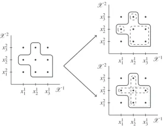
Fig. 4. Two possible decompositions of an event A into rectangular subsets.

appear. However, assuming that the collection

A

_n

_{= {}

A1

, . . . ,

An} over which the belief value Bel

(

Sn

i=1An)must be

evalu-ated contains only rectangular sets is not very restrictive, at least in the finite case. Indeed, any such set Ai

⊆ X

can then

be decomposed into a (non-unique) finite union of (not necessarily disjoint) rectangular subsets. To see this, note that there exists an elementary way to always achieve such a decomposition: one can always decompose A as the union of its

single-tons, each of them being a degenerate rectangular subset.Fig. 4illustrates two possible decompositions of the same subset

A. However, we shall see that such a decomposition is not always very interesting for applying the inclusion–exclusion

principle. The results of this section also provide conditions under which such a decomposition will allow one to apply the inclusion–exclusion principle.

3.1. Two sets, two dimensions

Let us first explore the case n

=

2 and D

=

2, that is

A

₂

_{= {}

A1

,

A2

}

with Ai

=

A1i

×

A2i for i

=

1

,

2. The main idea in this

case is that if A1

\

A2 and A2

\

A1 are rectangular with disjoint projections, then 2-additivity holds for belief functions, and

this property is characteristic.

Lemma 3. If A1and A2are rectangular and have disjoint projections on dimensions

X

1

, X

2, then there is no rectangular subset of

A1

∪

A2overlapping both A1and A2.

Proof. Consider C

=

C1

×

C2 overlapping both A1 and A2. So there is

(

a1

,

a2

) ∈

A1

∩

C and b1

×

b2

∈

A2

∩

C . Since C

is rectangular,

(

a1

,

b2

)

and

(

b1

,

a2

) ∈

C . However if C

⊆

A1

∪

A2 then

(

a1

,

b2

) ∈

A1

∪

A2 and either b2

∈

A21 or a1

∈

A12.

Since a1

_∈

_A1

1 and b2

∈

A22 by assumption, it would mean that projections of A1 and A2 are not disjoint, which leads to a

contradiction.

✷

We can now characterise under which conditions 2-additivity holds for belief functions.

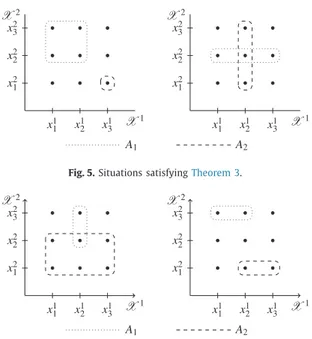
Theorem 3. 2-additivity applied to a proper family

A

₂

_{= {}

A1

,

A2

}

of rectangular sets holds for belief functions having rectangular

focal elements if and only if one of the following conditions holds

1. A1₁

∩

A1₂

=

A2₁

∩

A2₂

= ∅

,

2. A1

1

⊆

A12and A22

⊆

A21(or A11

⊇

A12and A22

⊇

A21, changing both inclusion directions).

Proof. First note that inclusions of Condition 2 can be considered as strict, as we have assumed A1

,

A2 to not be included

in each other, otherwise the result immediately follows from A1

∪

A2

=

A1if A1

⊆

A2or from A1

∪

A2

=

A2 if A2

⊆

A1.

⇐

:

1. If A1₁

∩

A1₂

=

A2₁

∩

A2₂

= ∅

, A1 and A2 are disjoint, as well as their projections. Then by Lemma 3, all rectangular

subsets included in A1

∪

A2 are either included in A1or in A2, henceLemma 1applies and 2-additivity holds for belief

functions.

2. A1

1

⊂

A12 and A22

⊂

A21 imply that A1

\

A2

=

A11

× (

A21

\

A22

)

and A2

\

A1

= (

A12

\

A11

) ×

A22. As A1

\

A2 and A2

\

A1 are

rectangular and have disjoint projections, Lemma 3 andLemma 1 apply (as above) and 2-additivity holds for belief

Fig. 5. Situations satisfyingTheorem 3.

Fig. 6. Situations not satisfyingTheorem 3.

⇒

:

1. Suppose A1

∩

A2

= ∅

with A11

∩

A12

6= ∅

(see right side ofFig. 6). Then

(

A11

∩

A12

) × (

A21

∪

A22

)

is rectangular, not contained

in A1 nor A2but contained in A1

∪

A2, showing that the focal element

(

A11

∩

A12

) × (

A21

∪

A22

)

does not satisfyLemma 1

and therefore that 2-additivity does not hold.

2. Suppose A1₁

⊂

A1₂ but A2₂

6⊂

A2₁ (see left side ofFig. 6). Again,

(

A1₁

∩

A1₂

) × (

A2₁

∪

A2₂

) =

A1₁

× (

A2₁

∪

A2₂

)

is rectangular,

neither contained in A1 nor A2 but contained in A1

∪

A2, hence 2-additivity does not hold.

✷

Figs. 5 and 6show various situations where conditions ofTheorem 3are satisfied and not satisfied, respectively.

3.2. The multidimensional case

We can now proceed to extendTheorem 3to the case of any number D of dimensions. However, this extension will not

be as straightforward as going fromLemma 1to Proposition 1, and we need first to characterise when the union of two

singletons is rectangular. We will call such rectangular unions minimal rectangles. A singleton is a degenerate example of a minimal rectangle.

Lemma 4. Leta

= (

a1

, . . . ,

aD

)

and b

= (

b1

, . . . ,

bD

)

be two distinct elements in

X

. Then,

{

a

,

b

}

forms a minimal rectangle if and only if there is only one i

∈ [

1

:

D

]

such that ai

6=

bi.

Proof.

⇒

: If ai

₆₌

_bi _{for only one i, then}

_{

_a

_,

_b

_{} = {}

_a1

_{} × . . . × {}

_ai

_,

_bi

_{} × . . . × {}

_aD

_}

_{is rectangular.}

⇐

: Let us now consider the case where ai

6=

bi and aj

6=

bjfor i

6=

j. In this case,

{

a

,

b

} =

©¡

a1

, . . . ,

ai

, . . . ,

aj

, . . . ,

aD

¢

,

¡

a1

, . . . ,

bi

, . . . ,

bj

, . . . ,

aD

¢ª

.

The projections of

{

a

,

b

}

on the dimensions of

X

are

{

ak

,

bk

}

, and we know that

{

ai

,

bi

}

as well as

{

aj

,

bj

}

, do not reduce to

singletons. Hence, the Cartesian product of the projections of

{

a

,

b

}

contains the set

{

a1

_{} × . . . × {}

_ai

_,

_bi

_{} × {}

_aj

_,

_bj

_{} × . . . × {}

_an

_}

_,

that contains elements not in

{

a

,

b

}

(e.g.

(

a1

_{, . . . ,}

_bi

_{, . . . ,}

_aj

_{, . . . ,}

_aD

₎

_{). Since}

_{

_a

_,

_b

_}

_{is not characterised by its projections on}

dimensions

X

_i, it is not rectangular, and this finishes the proof.

✷

As mentioned before, any set can be decomposed into rectangular sets, and in particular any rectangular set can be decomposed into minimal rectangles. Also, any rectangular set that is not a singleton will at least contain one minimal rectangle, implying that there always exist at least two singletons of a rectangular set forming a minimal rectangle (we will

use this in subsequent proofs). Let us now show howTheorem 3can be extended to D dimensions.

Theorem 4. 2-additivityholds for a proper family

A

₂

= {

A1

,

A2

}

of rectangular sets for belief functions having rectangular focal

1.

∃

distinct p

,

q

∈ {

1

, . . . ,

D

}

such that Ap₁

∩

Ap₂

=

Aq₁

∩

Aq₂

= ∅

,

2.

∀

i

∈ {

1

, . . . ,

D

}

either Ai₁

⊆

Ai₂or Ai₂

⊆

Ai₁.

Proof. Again, we can consider that there is at least two distinct p

,

q

∈ {

1

, . . . ,

D

}

such that inclusions A₁p

⊂

A₂pand Aq₂

⊂

Aq₁

of Condition 2 are strict, as we have assumed A1

,

A2 to not be included in each other (as inTheorem 3and for the same

reasons).

⇐

:

1. Any two a1

∈

A1 and a2

∈

A2 will be such that ai1

∈

Ai1 and ai2

∈

A2i must be distinct for i

=

p

,

q since A

p

1

∩

A

p

2

=

Aq₁

∩

Aq₂

= ∅

. By Lemma 4, this means that there is no pair a1

∈

A1 and a2

∈

A2 forming a minimal rectangle. This

implies that there is no minimal rectangle included in A1

∪

A2 overlapping A1 and A2, and therefore no rectangular

subset. It follows that each rectangular subset included in A1

∪

A2 is either included in A1 or in A2, henceLemma 1

applies and 2-additivity holds for belief functions.

2. Let us denote by P the set of indices p such that A₁p

⊂

Ap₂ and by Q the set of indices q such that Aq₂

⊂

Aq₁. Now, let

us consider two singletons a1

∈

A1

\

A2 and a2

∈

A2

\

A1. Then

• ∃

p

∈

P such that ap₁

∈

A₁p

\

A₂p, otherwise a1 is included in A1

∩

A2,

• ∃

q

∈

Q such that aq₂

∈

Aq₂

\

Aq₁, otherwise a2 is included in A1

∩

A2,

but since aq₁

∈

Aq₁ and a₂p

∈

A₂p by definition, a1and a2 must differ at least on two dimensions, hence byLemma 4one

cannot form a minimal rectangle outside A1

∩

A2, that is, by picking pairs of singletons in A1

\

A2 and A2

\

A1. As

above, this implies thatLemma 1is satisfied and that 2-additivity holds.

⇒

:

1. Suppose A1

∩

A2

= ∅

with Aq₁

∩

Aq₂

6= ∅

only for q. Then the following rectangular set contained in A1

∪

A2

¡

A1₁

∩

A1₂

¢ × . . . × ¡

A₁q−1

∩

Aq₂−1

¢ × ¡

Aq₁

∪

Aq₂

¢ × ¡

Aq₁+1

∩

A₂q+1

¢ × . . . × ¡

AD₁

∩

A₂D

¢

is neither contained in A1 nor A2, so 2-additivity will not hold (byLemma 1).

2. Suppose A1

∩

A2

6= ∅

and Aq₁

*

Aq₂, Aq₁

+

Aq₂ for some q. Again,

¡

A1₁

∩

A1₂

¢ × . . . × ¡

A₁q−1

∩

Aq₂−1

¢ × ¡

Aq₁

∪

Aq₂

¢ × ¡

Aq₁+1

∩

A₂q+1

¢ × . . . × ¡

AD₁

∩

A₂D

¢

is rectangular, neither contained in A1nor A2but contained in A1

∪

A2, so 2-additivity will not hold (byLemma 1).

✷

UsingProposition 1, the extension to n-additivity in D dimensions is straightforward:

Theorem 5. n-additivity holds for a proper family

A

_n

= {

A1

, . . . ,

An

}

of rectangular sets for belief functions having rectangular focal

elements if and only if, for each pair Ai,Aj, one of the following conditions holds

1.

∃

distinct p

,

q

∈ {

1

, . . . ,

D

}

such that Ap_i

∩

Ap_j

=

Aq_i

∩

Aq_j

= ∅

,

2.

∀ℓ ∈ {

1

, . . . ,

D

}

either Aℓ

i

⊆

Aℓjor Aℓj

⊆

Aℓi.

Note that the second condition is insensitive to set-complements, hence the following result:

Corollary 6. n-additivity holds on both

A

_n

_{= {}

A1

, . . . ,

An}and

A

n−

= {

Ac1

, . . . ,

Anc

}

for belief functions whenever for each pair Ai,Aj,

∀ℓ ∈ {

1

, . . . ,

D

}

either Aℓ

i

⊆

Aℓjor Aℓj

⊆

Aℓi.

3.3. On the practical importance of rectangular focal elements

While limiting ourselves to rectangular subsets in

A

is not especially restrictive, the assumption that focal elements

have to be restricted to rectangular sets may seem restrictive (as we are not free to cut any focal element into rectangular subsets). However, such mass assignments actually appear in many practical situations. They can result for example from

the combination of marginal masses mi _{defined on each dimension}

_X

i_{, i}

₌

₁

_{, . . . ,}

_{D under an assumption of (random set)}

independence[10]. In this case, the joint mass assigned to each rectangular set E is

m

(

E

) =

D

Y

i=1

mi

¡

Ei

¢

.

(10)

Additionally, the random set independence assumption makes the computation of the belief and plausibility functions of any rectangular set A easier, as they factorise in the following way:

Bel

(

A

) =

D

Y

i=1 Beli

¡

Ai

¢

,

(11) Pl

(

A

) =

D

Y

i=1 Pli

¡

Ai

¢

,

(12)

where Beli

,

Pliare the belief/plausibility measures induced by mi_.

An interesting fact is that since the proofs of Section3only require focal elements and events to be Cartesian products,

they also apply to the cases of unknown or partially known dependence, as long as these latter cases can be expressed by

linear constraints imposed on the joint mass[2]. Considering more generic models than belief functions is also possible, e.g.

lower probabilities. Then the positivity of the mass functions mino longer holds, but the approach can be carried out

with-out modifying our results since the product of (possibly negative) masses in such approaches preserves the approximation

properties of random set independence[13].

The following sections explore and discuss specific cases of interest where the inclusion–exclusion property applies. 4. The case of Boolean formulas

In this section, we explore the case where spaces

X

i _{are binary. In particular, conditions are laid bare for applying the}

inclusion–exclusion property to Boolean formulas expressed in Disjunctive Normal Form (DNF). We also discuss the problem of estimating plausibilities of Boolean formulas using the inclusion–exclusion property.

In propositional logic, each dimension

X

i_{is of the form}

_{

_xi

_{, ¬}

_xi

_}

_{. It can be associated to a Boolean variable also denoted}

by xi_{, and}

_X

1:D _{is also called the set of interpretations of the propositional language generated by the set of variables x}i_.

In this case, xi_{is understood as an atomic proposition, while}

_¬

_xi_{denotes its negation. An element of}

_X

i_{is called a literal}

(xi is a positive one and

¬

xi a negative one). Any rectangular set A

⊆ X

1:D _{can then be interpreted as a conjunction of}

literals (it is often called a partial model), and given a collection of n such partial models

A

_n

= {

A1

, . . . ,

An}, the event

A1

∪ . . . ∪

An is a Boolean formula expressed in Disjunctive Normal Form (DNF – a disjunction of conjunctions). All Boolean

formulas can be written in such a form.

A convenient representation of a partial model A is in the form of an orthopair[8]

(

P

,

N

)

of disjoint subsets of indices

of variables P

,

N

⊆ [

1

:

D

]

such that A(P,N)

=

V

k∈Pxk

∧

V

k∈N

¬

xk. Then an element in

X

1:D is of the form

V

k∈Pxk

∧

V

k∈Pc

¬

xk, i.e. corresponds to an orthopair

(

P

,

Pc

)

.

We consider belief functions generated by focal elements having the form of partial models. To this end, we consider

that the uncertainty over each Boolean variable xi _{is described by a belief function Bel}i_{. As}

_X

i_{is binary, its mass function}

mi only needs two numbers to be defined. Indeed, it is enough to know li

=

Beli

({

xi

})

and ui

=

Pli

({

xi

}) ≥

li (for instance a

probability interval[11]) to characterise the marginal mass function misince:

•

Beli

({

xi

_{}) =}

_li

₌

_mi

_({

_xi

_})

_;

•

Pli

({

xi

}) =

1

−

Beli

({¬

xi

}) =

ui

⇒

mi

({¬

xi

}) =

Beli

({¬

xi

}) =

1

−

ui;

•

The sum of masses is mi

({

xi

}) +

mi

({¬

xi

}) +

mi

(X

i

) =

1, so mi

(X

i

) =

ui

−

li.

Given D independent marginal masses mi _on

_X

i_{, i}

₌

₁

_{, . . . ,}

_{D, the joint mass m on}

_X

1:D _{can be computed as follows}

for any partial model A(P,N), applying Eq.(10):

m

(

A(P,N)) =

µ

Y

i∈P li

¶µ

Y

i∈N

(

1

−

ui

)

¶µ

Y

i∈/P∪N

(

ui

−

li

)

¶

.

(13)

We can then give explicit expressions for the belief and plausibility of conjunctions or disjunctions of literals in terms of marginal mass functions:

Proposition 7. Thebelief of a conjunction C(P,N)

=

V

k∈Pxk

∧

V

k∈N

¬

xk, and that of a disjunction D(P,N)

=

W

k∈Pxk

∨

W

k∈N

¬

xkof

literals forming an orthopair

(

P

,

N

)

are respectively given by:

Bel

(

C(P,N)) =

Y

i∈P li

Y

i∈N

¡

1

−

ui

¢

,

(14) Bel

(

D(P,N)) =1

−

Y

i∈P

¡

1

−

li

¢ Y

i∈N ui

.

(15)

Proof. Bel

(

C(P,N)

)

can be obtained by applying Eq.(11)to C(P,N).

Pl

(

C(N,P)) =Pl

µ

^

i∈N xi

∧

^

i∈P

¬

xi

¶

=

Y

i∈N

¡

1

−

li

¢ Y

i∈P ui

=

1

−

µ

1

−

Y

i∈N

(

1

−

li

)

Y

i∈P ui

¶

=

1

−

Bel

µ

_

i∈N

¬

xi

∨

_

i∈P xi

¶

=

1

−

Bel

(

D(P,N))

with the second equality following from Eq.(12).

✷

Using the fact that Bel

(

C(N,P)

) =

1

−

Pl

(

D(P,N)

)

, we can deduce

Pl

(

D(P,N)) =1

−

Y

i∈P li

Y

i∈N

¡

1

−

ui

¢

.

We can particularise Theorem 5 to the case of Boolean formulas, and identify conditions under which the belief or

the plausibility of a DNF can be easily estimated using the inclusion–exclusion Equality(1). Let us see how the conditions

exhibited in this theorem can be expressed in the Boolean case.

Consider the first condition ofTheorem 5

∃

p

6=

q

∈ {

1

, . . . ,

D

}

such that A_ip

∩

Ap_j

=

Aq_i

∩

Aq_j

= ∅.

Note that when spaces are binary, Ap_i

= {

xp

_}

_{(if p}

_∈

_P

i), or Aip

= {¬

xp

}

(if p

∈

Ni), or yet Aip

= X

i(if p

∈

/

Pi

∪

Ni). Ai

∩

Aj

= ∅

therefore means that for some index p, p

∈ (

Pi

∩

Nj) ∪ (Pj

∩

Ni)(there are two opposite literals in the conjunction).

The condition can thus be rewritten as follows, using orthopairs

(

Pi,Ni)and

(

Pj,Nj):

∃

p

6=

q

∈ {

1

, . . . ,

D

}

such that p

,

q

∈ (

Pi

∩

Nj

) ∪ (

Pj

∩

Ni

).

Example 1. Consider the equivalence connective x1

⇔

x2

= (

x1

∧

x2

) ∨ (¬

x1

∧ ¬

x2

)

so that A1

=

x1

∧

x2 and A2

= ¬

x1

∧ ¬

x2.

We have P1

= {

1

,

2

},

N1

= ∅,

P2

= ∅,

N2

= {

1

,

2

}

. So, p

=

1

∈

P1

∩

N2

,

q

=

2

∈

P1

∩

N2, hence the condition is satisfied and

Bel

(

x1

_⇔

_x2

_{) =}

_Bel

₍

_x1

_∧

_x2

_{) +}

_Bel

_(¬

_x1

_{∧ ¬}

_x2

₎

_{(the remaining term is Bel}

_(∅)

_).

Likewise, the exclusive or: x1

⊕

x2

= (

x1

∧ ¬

x2

) ∨ (¬

x1

∧

x2

)

so that A1

=

x1

∧ ¬

x2 and A2

= ¬

x1

∧

x2. We have P1

=

{

1

},

N1

= {

2

},

P2

= {

2

},

N2

= {

2

}

. So, p

=

1

∈

P1

∩

N2

,

q

=

2

∈

N1

∩

P2and Bel

(

x1

⊕

x2

) =

Bel

(

x1

∧ ¬

x2

) +

Bel

(¬

x1

∧

x2

)

(again,

the remaining term is Bel

(∅)

).

The second condition ofTheorem 5reads

∀ℓ ∈ {

1

, . . . ,

D

}

either Aℓ_i

⊆

Aℓ_j or Aℓ_j

⊆

Aℓ_i

and the condition Aℓ_i

⊆

Aℓ_j can be expressed in the Boolean case as:

ℓ ∈

¡

Pi

∩

Ncj

¢ ∪ ¡

Ni

∩

Pcj

¢ ∪ ¡

Pci

∩

Nci

∩

Pcj

∩

Ncj

¢

.

The condition can thus be rewritten as follows, using orthopairs

(

Pi,Ni)and

(

Pj,Nj):

Pi

∩

Nj

= ∅

and Pj

∩

Ni

= ∅

Example 2. Consider the disjunction x1

∨

x2, where A1

=

x1 and A2

=

x2, so that P1

= {

1

},

P2

= {

2

},

N1

=

N2

= ∅

. So

Bel

(

x1

_∨

_x2

_{) =}

_Bel

₍

_x1

_{) +}

_Bel

₍

_x2

_{) −}

_Bel

₍

_x1

_∧

_x2

₎

_{. Likewise for implication, x}1

_→

_x2

_{= ¬}

_x1

_∨

_x2_{, where A}

1

= ¬

x1 and A2

=

x2, so

that N1

= {

1

},

P2

= {

2

},

P1

=

N2

= ∅

. So Bel

(

x1

→

x2

) =

Bel

(¬

x1

) +

Bel

(

x2

) −

Bel

(¬

x1

∧

x2

)

. We can summarise the above results as

Proposition 8. Theset of partial models

A

_n

= {

A1

, . . . ,

An}satisfies the inclusion–exclusion principle if and only if, for any pair Ai,Aj

one of the two following conditions is satisfied:

• ∃

p

6=

q

∈ {

1

, . . . ,

D

}

such that p

,

q

∈ (

Pi

∩

Nj) ∪ (Pj

∩

Ni).

•

Pi

∩

Nj

= ∅

and Pj

∩

Ni

= ∅

.

This condition tells us that for any pair of partial models:

•

either conjunctions Ai,Aj contain at least two opposite literals,

•

or events Ai,Aj have a non-empty intersection and have a common model.

As a consequence we can compute the belief of any logical formula that obeys the conditions ofProposition 8in terms

of the belief and plausibilities of atoms xi.

Example 3. Consider the formula

(

x1

∧ ¬

x2

) ∨ (¬

x1

∧

x2

) ∨

x3, with A1

=

x1

∧ ¬

x2, A2

= ¬

x1

∧

x2, A3

=

x3. We have

P1

= {

1

},

N1

= {

2

},

P2

= {

2

},

N2

= {

1

},

P3

= {

3

},

N3

= ∅

. Thus it satisfiesProposition 8, and

Bel

¡¡

x1

∧ ¬

x2

¢ ∨ ¡¬

x1

∧

x2

¢ ∨

x3

¢

=

Bel

¡

x1

∧ ¬

x2

¢ +

Bel

¡¬

x1

∧

x2

¢ +

Bel

¡

x3

¢ −

Bel

¡

x1

∧ ¬

x2

∧

x3

¢ −

Bel

¡¬

x1

∧

x2

∧

x3

¢

(other belief values are equal to 0 since referring to contradictory Boolean expressions)

=

l1

(

1

−

u2

) + (

1

−

u1

)

l2

+

l3

¡

1

−

l1

(

1

−

u2

) − (

1

−

u1

)

l2

¢

The conditions ofProposition 8allow us to check, once a formula has been put in DNF, whether or not the inclusion–

exclusion principle applies. Important particular cases where it applies are disjunctions of partial models Ci having only

positive (resp. negative) literals, of the form C1

∨ ... ∨

Cn, where N1

= . . . =

Nn

= ∅

(resp. P1

= . . . =

Pn

= ∅

). This is the

typical Boolean formula obtained in fault tree analysis, where elementary failures are modelled by positive literals, and the

general failure event is due to the simultaneous occurrence of some subsets of elementary failures (see Section6.1). Namely,

we have Bel

(

C1

∨ ... ∨

Cn

) =

n

X

i=1 Bel

(

Ci

) −

n−1

X

i=1 n

X

j=i+1 Bel

(

Ci

∧

Cj

)

+

n−2

X

i=1 n−1

X

j=i+1 n

X

k=j+1 Bel

(

Ci

∧

Cj

∧

Ck

) − ... + (−

1

)

m+1Bel

(

C1

∧ ... ∧

Cn

),

(16)

where the terms on the right-hand side can be computed from belief values of atoms as Bel

(

C(P,∅)

) =

Q

i∈Plias per

Propo-sition 7.

More generally, the inclusion–exclusion principle applies to disjunctions of partial models which can, via a renaming, be rewritten as a disjunction of conjunctions of positive literals: namely, whenever a single variable never appears in a positive

and negative form in two of the conjunctions. This is equivalent to the second condition ofProposition 8. Then, of course,

values 1

−

ui _{must be used in place of l}i_{for negative literals.}

For such Boolean formulas, the inclusion–exclusion principle can also be used to also estimate the plausibility of

C1

∨ ... ∨

Cn. Indeed, consider the formula

W

i∈[1:n]

(

V

k∈Pix

i

)

possibly obtained after a renaming, then

¬

µ

_

i∈[1:n]

µ

^

k∈Pi xi

¶¶

=

^

i∈[1:n]

¬

µ

^

j∈Pi xj

¶

=

^

i∈[1:n]

_

j∈Pi

¬

xj

=

_

E k∈P1×...×Pn

^

j∈[1:n]

¬

xkj

using distributivity, where

E

k ranges on n-tuples of indices (one component per conjunction Ci). Namely, starting with a DNF

involving conjunctions of positive literals,

V

_i∈[1:n]

W

_j∈P

i

¬

x

j _{is turned into a DNF with only negative literals, to which the}

second condition ofProposition 8applies, and

Pl

µ

_

i∈[1:n]

µ

^

k∈Pi xi

¶¶

=

1

−

Bel

µ

_

E k∈P1×...×Pn]

^

j∈[1:n]

¬

xki

¶

.

On the other hand, it is not always possible to put the complement of every formula satisfying the second condition of

Example 4. Consider the equivalence formula between three elements, that is the formula F

= (¬

x1

∧ ¬

x2

∧ ¬

x3

) ∨ (

x1

_∧

x2

∧

x3

)

. It satisfiesProposition 8, but its negation

¬

F

=

¡

x1

∧ ¬

x2

¢ ∨ ¡

x2

∧ ¬

x3

¢ ∨ ¡

x3

∧ ¬

x1

¢

,

(17)

once put in DNF form, does not satisfyProposition 8(each pair of conjunctions possesses only one variable with opposite

literal). However, the negation of other formulas such as logical equivalence between two elements possesses a DNF form

¬(

x1

⇔

x2

) = (

x1

∧ ¬

x2

) ∨ (¬

x1

∧

x2

)

that satisfiesProposition 8.

Example 5. As another example where the inclusion–exclusion principle cannot be applied, consider the formula x1

∨ (¬

x1

_∧

x2

₎

_{(which is just the disjunction x}1

_∨

_x2_{we already considered above). It does not hold that Bel}

₍

_x1

_{∨ (¬}

_x1

_∧

_x2

_{)) =}

_Bel

₍

_x1

_{) +}

Bel

(¬

x1

∧

x2

) =

l1

+ (

1

−

u1

)

l2. Indeed the latter sum neglects m

(

x2

) = (

u1

−

l1

)

l2, since x2 is a focal element that implies

x1

∨

x2 but neither x1 nor

¬

x1

∧

x2. However, computing Bel

(

x1

∨

x2

)

is obvious as 1

− (

1

−

l1

)(

1

−

l2

)

fromProposition 7.

The last remark suggests that normal forms that are very useful to compute the probability of a Boolean formula

ef-ficiently, such as BDD[6]may be useless to speed up the computation of its belief and plausibility degrees. For instance,

x1

∨ (¬

x1

∧

x2

)

is a binary decision diagram (BDD) for the disjunction, and this form prevents Bel

(

x1

∨

x2

)

from being

properly computed by standard methods as the inclusion–exclusion principle fails in this case. The question whether any

Boolean formula can be re-expressed in a form satisfyingProposition 8is answered to the negative by Formula(17), which

provides a counterexample to this claim.

5. The case of events defined by monotone functions

In this section, we show that the inclusion–exclusion principle can be applied to evaluate some events of interest defined by means of monotone functions on Cartesian products of discrete linearly ordered spaces. Such functions are commonly

used in problems such as multi-criteria decision making[20], reliability assessments[14]or optimisation problems[19].

We assume that we have some function

φ : X

1:D

→ Y

where variables xj, j

=

1

, . . . ,

D take their values on a finite

linearly ordered space

X

j

= {

x₁j

, . . . ,

x_kj

j

}

of kjelements. We denote by

≤

jthe order relation on

X

j and assume (without

loss of generality) that elements are indexed such that x_ij

<

jxkjiff i

<

k. We also assume that the output space

Y

is ordered

and we denote by

≤

Y the order on

Y

, assuming an indexing such that yi

<

Y ykiff i

<

k. Given two elements x

,

z

∈ X

1:D,

we simply write x

≤

z if xj

≤

jzjfor j

=

1

, . . . ,

n, and x

<

z if moreover xj

<

jzj for at least one j.

We assume that the function is non-decreasing in each of its variables xj_{, that is}

φ

¡

x1_i 1

, . . . ,

x ℓ iℓ

, . . . ,

x D iD

¢ ≤Y

φ

¡

x1_i 1

, . . . ,

x ℓ i′ ℓ

, . . . ,

x_iD D

¢

(18)

iff iℓ

≤

i′_ℓ. Note that a function monotone in each variable xj can always be transformed into a non-decreasing one, since if

φ

is decreasing in Xi, it becomes non-decreasing in xiwhen considering the reverse ordering of

≤

j (i.e., xij

<

x

j

kiff k

<

i).

We now consider the problem where we want to estimate the uncertainty of some event

{φ ≥

d

}

(or

{φ <

d

}

, that can be

obtained by duality). Evaluating the uncertainty over such events is instrumental in a number of applications, from checking

whether a threshold can be trespassed in risk analysis[3]to computing level sets when solving the Choquet integral, e.g.,

in multi-criteria decision making [20]. Given a value d

∈ Y

, let us define the concept of minimal path and minimal cut

vectors.

Definition 1. A minimal path (MP) vector p for value d, induced by a function

φ

, is an element p

∈ X

1:D _{such that}

_{φ (}

_p

_{) ≥}

_d

and

φ (

y

) <

d for any y

<

p.

Definition 2. A minimal cut (MC) vector c for value d, induced by a function

φ

, is an element c

∈ X

1:D _{such that}

φ (

c

) <

d

and

φ (

y

) ≥

d for any y

>

c.

Let

{

p1

, . . . ,

pn}be the set of all minimal path vectors of some function

φ

for a given threshold demand d. We denote

by Api

= {

x

∈ X

1:D

_|

_x

_≥

_{pi}the event corresponding to the set of configurations dominating the minimal path vector p}

iand

by

A

_n

= {

Ap1

, . . . ,

Apn

}

the set of events induced by minimal path vectors. Note that each set

Api

= ×

D j=1

©

xj

¯

¯

xj

≥

jp_ij

ª

(19)

is rectangular, hence we can use results from Section3.