FEDERICO TORRIANO
INVESTIGATION OF THE 3D FLOW
CHARACTERISTICS IN A ROTATING
CHANNEL SETUP
Mémoire présente
à la Faculté des études supérieures de l'Université Laval dans le cadre du programme de maîtrise en génie mécanique
pour l'obtention du grade de maître es sciences (M.Se.)
FACULTE DES SCIENCES ET DE GENIE UNIVERSITÉ LAVAL
QUÉBEC
OCTOBRE 2006
L'objectif de ce projet de maîtrise est de contribuer à une meilleure compréhension des écoulements dans les conduits rectangulaires en rotation. Une attention particulière est apportée aux effets de bout et au développement de l'écoulement.
Des simulations RANS en régime stationnaire ont démontré que la présence d'un écoulement secondaire de faible intensité est suffisante pour modifier le profil de vitesse axiale de façon à que ce dernier diffère significativement de la solution théorique 2D. En conséquence, les comparaisons entre les résultats expérimentaux et les simulations numériques 2D devraient être faites avec prudence.
Les calculs stationnaires ont également montré que le développement de l'écoulement dans un canal tournant est affecté par l'apparition de cellules de type Taylor-Gôrtler le long du mur pression. Puisque ces tourbillons sont légèrement inclinés par rapport au plan horizontal, une solution stationnaire pleinement développée n'est jamais atteinte. Des simulations subséquentes en régime instationnaire dans un domaine périodique ont prouvé qu'une solution pleinement développée peut cependant exister dans un canal tournant, mais l'écoulement est alors formellement instationnaire car les cellules lon-gitudinales sont convectées vers les bouts de la conduite par l'action de l'écoulement secondaire.
Abstract
The objective of the présent work is to provide a basic description and to contribute toward a better understanding of rotating high aspect ratio duct flows. Particular attention is given to end-wall effects and flow development.
Steady RANS simulations hâve shown that the présence of a weak, but unavoidable, end-wall generated secondary flow produces suffîcient transverse advection to alter the streamwise velocity profile in such a way that it differs noticeably from the theoretical 2D channel case. Thus, comparisons between expérimental results and 2D numerical simulations should be performed very cautiously.
Steady state calculations hâve also revealed that the flow development in a rotating duct is subtly affected by the appearance of longitudinal Taylor-Gortler type cells near the pressure wall. Since the roll cells are tilted toward the end-wall, no steady fully developed solution is ever reached.
Subséquent unsteady flow calculation in a streamwise periodic domain hâve shown that a fully developed solution can exist in a rotating duct, but the resulting flow field is formally unsteady due to the convection of the roll cells toward the end-wall.
J'aimerais d'abord remercier mon directeur de recherche, le professeur Guy Dumas. Ses précieux conseils et son ample expertise dans le domaine de la mécanique des flu-ides numérique m'ont permis de mener à terme le projet de maîtrise et d'acquérir des bonnes connaissances de base en CFD. Je tiens également à souligner la contribution du professeur Yvan Maciel car son expertise dans le domaine des écoulements en repère tournant a grandement contribué au bon déroulement de mes recherches.
Je voudrais aussi souligner le soutien financier du Conseil de Recherche en Sciences Na-turelles et Génie (CRSNG) du Canada et la contribution, via son programme de bourses, du Fond Québécois de la Recherche sur la Nature et les Technologies (FQRNT). Leur appui financier a été grandement apprécié.
Je souhaiterais également exprimer ma profonde gratitude à Steve Julien avec qui j'ai partagé une grande partie du projet de recherche. Je profite également de cette occasion pour saluer tous les étudiants membres du LMFN et en particulier Florian, Thomas, Julie, Pascal, Félix-Antoine et Pierre-Luc.
En dernier lieu, je veux exprimer ma plus grande gratitude à mes parents à qui ce travail est dédié.
A tutta la mia famiglia
Résumé ii Abstract iii Avant-propos iv Contents vi List of Tables viii List of Figures ix 1 Introduction 1 1.1 Preliminaries 1 1.2 Objectives 3 1.3 Methodology 3 2 Theoretical background 4 2.1 Governing équations 4 2.2 Flow phenomena in a rotating channel 5 2.3 Flow phenomena in a rotating duct 7 2.4 Flow phenomena in a bend 10
3 Numerical method 12
3.1 Fluent: a finite volume solver 12 3.2 RANS approach to turbulent flows 13 3.3 Wall treatment 17 3.4 Numerical schemes 19
4 Validation efforts 21
4.1 Validation of the turbulence model and wall treatment 21 4.2 Validation of the boundary conditions 25
Contents vii
5.1 Fully developed flow in a rotating channel 32 5.2 Fully developed flow in a rotating duct 36 5.2.1 Mesh independence 37 5.2.2 End-wall effects on two-dimensionality 41 5.2.3 Reynolds and Rotation number effects 46 5.2.4 Comparison between expérimental and DNS data 52
6 Flow development in a rotating channel 54
6.1 Effect of rotation on flow development 54 6.1.1 Mesh independence 55 6.1.2 Flow development in a rotating and non-rotating channel . . . . 57 6.2 Validation of the design hypothesis 61 6.3 Improvements on the actual design 69
7 Flow development in a rotating duct 74
7.1 Effect of rotation on flow development 74 7.1.1 Mesh independence 74 7.1.2 Flow development in a rotating and non-rotating duct 77 7.1.3 Effect of mesh discretization on roll cell instability 84 7.1.4 Effect of roll cell instability on flow development 87 7.2 Validation of the design hypothesis 90 7.3 Improvements on the actual design 99
8 Unsteady fully developed flow in a rotating duct 105
8.1 Unsteady calculation in a rotating duct of finite aspect ratio 105 8.2 Unsteady calculation in a rotating duct of infinité aspect ratio 1.10
9 Conclusion 112 Bibliography 115 A Fully developed solution with periodic boundary conditions 118 B Tested designs for promoting flow development 122
B.l Actual channel without splitter plate 1.22 B.2 Actual channel with symmetric lips 123 B.3 Actual channel with symmetric lips and flaps 124 B.4 Actual channel with symmetric lips, flaps and filters 125 C Parallel solver performance 127
4.1 Comparaison of non-rotating case - Re = 6210 22 4.2 Comparaison of rotating case - Re = 6899 at Ro = 0.2 22 4.3 ||AL=100h||RMs values in a yz plane of a rotating duct at two measurement
stations - Re = 40000 and Ro = 0.22 29 5.1 Rotation effect on wall shear stress at Re — 40000 34 5.2 Reynolds effect on wall shear stress at Ro = 0.22 34 5.3 ||A||RMS values in the central yz plane of a rotating duct at Re = 40000 and
Ro = 0.22 40
5.4 ||A||HMS values at symmetry axis of a rotating duct at Re = 40000 and
# 0 = 0.22 40 5.5 ||Aî / h = 0||R M S values of streamwise velocity at différent spanwise locations (from
symmetry plane at z/h = 0 toward the end wall of a rotating and non-rotating duct at Re = 40000 45 5.6 || A2D || HMS values of streamwise velocity at différent locations of a rotating and
non-rotating duct at Re = 40000 45 5.7 ||A2 D||HMS values of streamwise velocity at the symmetry plane of a rotating
duct at Ro = 0.22 52 6.1 || A||BMS values at différent stations along a rotating channel at Re = 40000
and Ro = 0.22 55 7.1 ||A||BMS values at différent stations along a duct at Re = 40000 and Ro = 0. 77
A.l ||A||KMS values at the central position of a periodic domain 118
A.2 2D channel at Re — 40000 and Ro = 0. Maximum variable fluctuations along a line at y/h = —0.5 121 C l Computational time of sériai and parallel solvers 127 C.2 Computational gain from parallel solver 128 C.3 Computational gain from parallel solver 1.28
List of Figures
1.1 Expérimental setup. (a): top view; (b): side view. From Maciel et al. (2003). 2 1.2 Expérimental results (Maciel et ai, 2003). (a): Mean streamwise velocity
profiles at ReT sa 180. D,x/h = 80; A,x/h - 118; - —, DNS (Alvelius et al,
1999). (b): R.m.s. streamwise velocity fluctuations at ReT « 180, symbols as
in (a) 2 2.1 Rotating turbulent channel flow. , Streamwise velocity profile for Ro > 0;
, streamwise velocity profile for Ro = 0 6 2.2 Secondary flow génération in a rotating duct S 2.3 Roll cells instability in rotating duct flow. Light gray contours: u>x > 0; dark
gray: LÛX < 0 9
2.4 Détails of the expérimental setup configuration. Secondary flow génération in a bend (Dean-type cells) 11 3.1 Velocity profile as a function of distance normal to the wall. • , Expérimental
data; , wall functions. From Ferziger & Peric, 2002 17 3.2 Wall function approach 18 3.3 Finite volume approach for a Cartesian 2D grid. From Ferziger &; Peric, 1992. 20 4.1 Coarse mesh for rotating case 22 4.2 Mean velocity profiles in wall coordinates for différent rotation rates (0 <
Ro < 0.50) at Re = 2900. From Kristoffersen & Andersson, 1993 23 4.3 Normalized mean velocity profiles and Reynolds stress components. • , Coarse
mesh; A, fine mesh; , DNS by Alvelius. (a): Re = 6210 at Ro — 0; (b): Re = 6899 at Ro = 0.20 24 4.4 Normalized mean velocity profiles and Reynolds stress components at Re =
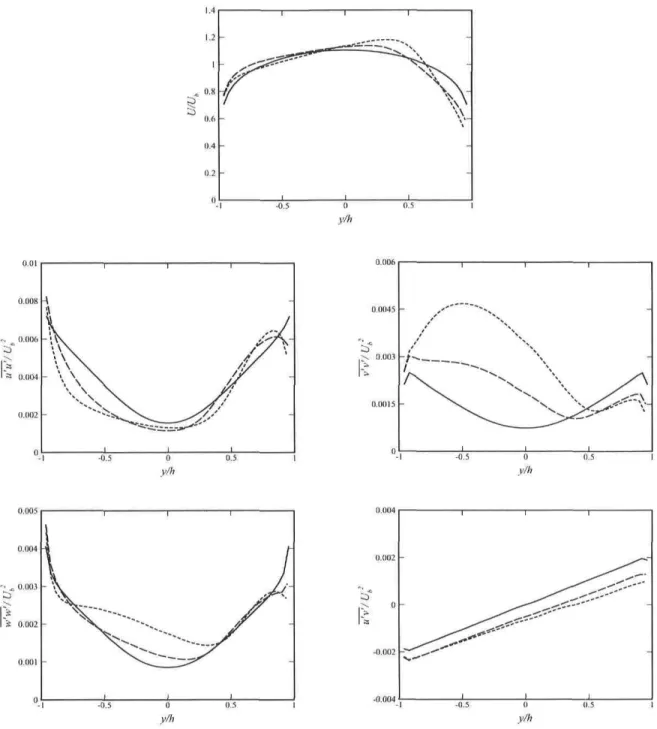
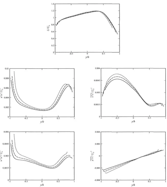
40000 and Ro = 0.22. D, Domain of length 60/i; , domain of length lOO/i. (a): Measurement station at x/h = 50 (lO/i from exit boundary of shorter domain); (b): measurement station at x/h = 60 (at exit boundary of shorter domain) 27
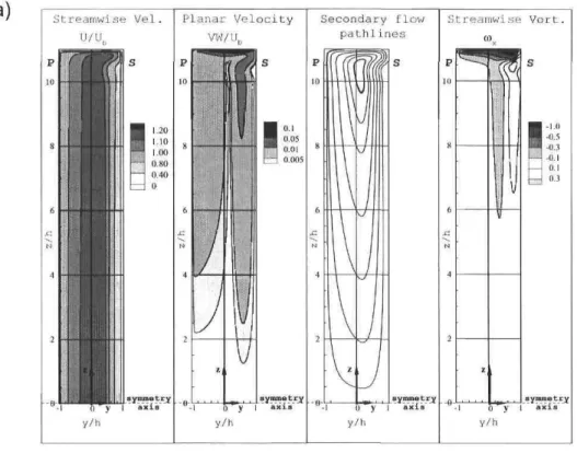
4.5 Plane contours in a rotating duct at Re = 40000 and Ro = 0.22. Flow direction toward the observer, (a): Measurement station at x/h = 50 (lOh from exit boundary of shorter domain); (b): measurement station at x/h = 60 (at exit boundary of shorter domain). Top figures correspond to the short domain while bottom ones correspond to the long domain 28 4.6 Fully developed solution in a rotating duct at Re = 40000 and Ro = 0.22.
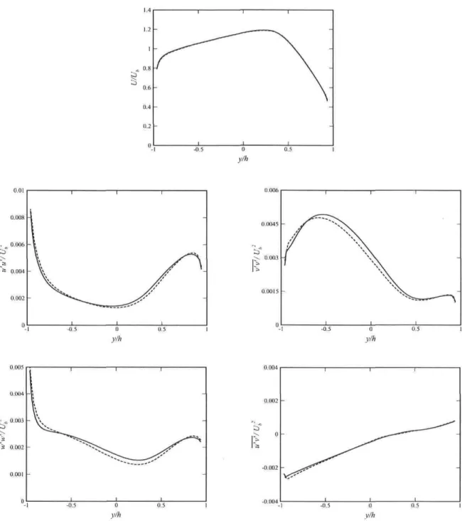
Normalized mean velocity profiles and Reynolds stress components along a Une placed at x/h = 0 and z/h = 0. D, Domain with symmetry condition;
—, whole domain 30 4.7 Fully developed solution in a rotating duct at Re = 40000 and Ro — 0.22.
Normalized mean velocity profiles and Reynolds stress components along a line placed at x/h = 0 and z/h = 2. D, Domain with symmetry condition;
—, whole domain 31 5.1 Fully developed solution in a rotating channel at Re = 40000. Normalized
mean streamwise velocity and Reynolds stress components. , Ro = 0; —,
Ro = 0.11; - - -, Ro = 0.22 33
5.2 Fully developed solution in a rotating channel at Ro = 0.22. Normalized mean streamwise velocity and Reynolds stress components. , Re = 40000; ,
Re = 20000; , Re = 10000 35
5.3 (a): Computational domain of'3D fully developed duct. (b): Mesh distribution in the yz plane; size of wall-adjacent cells corresponds to case at Re = 40000 and Ro = 0.22 37 5.4 Plane contours of a rotating duct at Re = 40000 and Ro = 0.22. (a): Standard
mesh; (b): fine mesh. Flow direction toward the observer 38 5.5 Profiles at symmetry axis of a rotating duct at Re = 40000 and Ro = 0.22.
—, Fine mesh; —, standard mesh 39 5.6 End-wall effects in a rotating duct at Re = 40000 and Ro = 0.22. Flow
direction toward the observer 41 5.7 Velocity and Reynolds stress profiles of a rotating duct/channel at Re = 40000
and Ro = 0.22. , 3D case (at symmetry plane); — , 2D case. Um is the
mean velocity at the symmetry plane 42 5.8 Turbulence and secondary flow contributions to the ar-momentum équation at
the symmetry plane of a rotating duct (thin lines) and rotating channel (thick line); Re = 40000 and Ro = 0.22 43 5.9 Velocity profiles at différent spanwise locations of a duct at Re = 40000:
z/h = 0, z/h = 2, z/h = 4, z/h = 6, z/h = 8, z/h = 10. (a): Ro = 0.22;
(b): Ro = 0. , 3D case; —, 2D case. The direction of the arrows indicates increasing z 44 5.10 Plane contours of a duct at Re = 40000. (a): Ro = 0.11; (b): Ro = 0. Flow
List of Figures xi
5.11 Velocity and Reynolds stress profiles of a duct and channel at Re = 40000. —, 3D case (at symmetry plane); — , 2D case. Um is the mean velocity at
the symmetry plane 48 5.12 Turbulence and secondary flow contributions to the z-momentum équation at
the symmetry plane of a rotating duct at Ro = 0.22. Black lines: Re — 40000; red lines: Re = 20000; green lines: Re = 10000 49 5.13 Plane contours of a duct at Ro = 0.22. (a): Re = 20000; (b): Re = 10000.
Flow direction toward the observer 50 5.14 Velocity and Reynolds stress profiles of a duct and channel at Ro = 0.22. - —,
3D case (at symmetry plane); — , 2D case. Um is the mean velocity at the
symmetry plane 51 5.15 Expérimental streamwise velocity profile at the symmetry plane of a
rotat-ing duct at Re = 2897 and Ro = 0.22 (Maciel et al, 2003). U,x/h = 80; Q,x/h = 135; - -, DNS (Alvelius et al, 1999) 53 6.1 Standard mesh for studying the flow development in a rotating channel at
Re = 40000 and Ro = 0.22 55
6.2 Streamwise velocity and turbulent viscosity ratio profiles at différent stations along a rotating channel at Re = 40000 and Ro = 0.22. —, Fine mesh;
-, standard mesh 56 6.3 Streamwise velocity profiles at différent stations along a channel at Re — 40000.
—, Solution at measurement station; - -, fully developed solution, (a):
Ro = 0; (b): Ro = 0.22. (c): ||AFD||RMS norm of the différence 58
6.4 Turbulent viscosity ratio profiles at différent stations along a channel at Re = 40000. —, Solution at measurement station; - -, fully developed solution.
(a): Ro = 0; (b): Ro = 0.22. (c): ||AFD||KMS norm of the différence 61
6.5 (a): Top view of expérimental setup; (b): 2D computational domain 62 6.6 Inlet section of computational domain. Mesh discretization for case study at
Re = 40000 and Ro = 0.22 63
6.7 Streamwise velocity profiles and ||AFD||RMS values at différent stations along a
rotating channel at Ro = 0.22. , Straight channel; - —, actual channel; -, fully developed solution, (a): Re = 40000; (b): Re = 20000 64 6.8 Streamlines in the entrance région of the actual channel at Ro — 0.22. (a):
Re = 40000; (b): Re = 20000 65
6.9 Turbulent viscosity ratio profiles at différent stations along a rotating channel at Ro = 0.22. —, Straight channel; - —, actual channel; - -, fully developed solution, (a): Re = 40000; (b): Re = 20000 66 6.10 Streamwise velocity profiles and ||AFD||RMS values at différent stations along a
rotating channel at Ro = 0.22. , Straight channel; - —, actual channel; -, fully developed solution, (a): Re = 40000; (b): Re = 20000 67
6.11 Streamlines in the entrance région of the actual channel at Ro = 0.22. (a): Re = 40000; (b): Re = 20000 68 6.12 Inlet section of computational domain. Mesh discretization for case study at
Re = 40000 and Ro = 0.22 69 6.13 Streamlines in the entrance région of the modified channel at Ro = 0.22.
(a): Re = 40000; (b): Re = 20000 70 6.14 Streamwise velocity profiles and ||AFD||RMS values at différent stations along a
rotating channel at Ro = 0.22. , Actual channel; - —, modified channel; -, fully developed solution, (a): Re = 40000; (b): Re = 20000 7.1 6.15 Turbulent viscosity ratio profiles at différent stations along a rotating chanriel
at Ro = 0.22. —, Actual channel; - —, modified channel; - -, fully developed solution, (a): Re = 40000; (b): Re = 20000 72 7.1 Coarse and refined meshes for studying the flow development in a non-rotating
duct at Re = 40000 75 7.2 Flow development in a duct at Re = 40000 and Ro = 0. Plane contours at
x/h = 140. (a): Standard mesh; (b): fine mesh. Flow direction toward the observer 76 7.3 Evolution of the mean velocity at the symmetry plane of a duct at
Re = 40000 78 7.4 Streamwise velocity profiles (normalized with the bulk velocity) at symmetry
plane of a duct at Re = 40000. - —, Solution at measurement station; -, fully developed solution, (a): Ro = 0; (b): Ro = 0.22. (c): ||AFD||RMS norm of the différence 80 7.5 Streamwise velocity profiles (normalized with the mean velocity) at symmetry
plane of a duct at Re = 40000. —, Solution at measurement station; -, fully developed solution, (a): Ro = 0; (b): Ro = 0.22. (c): ||AFD||BMs norm of the différence 81 7.6 Plane contours at différent stations along a duct at Re = 40000. (a): Ro = 0;
(b): Ro = 0.22. Flow direction toward the observer 82 7.7 Flow development processes in a finite aspect ratio rotating duct 83 7.8 Transverse velocity profiles at symmetry plane of a duct at Re = 40000 and
Ro = 0.22. , Solution at measurement station; — , fully developed solution. (a): Coarse mesh; (b): fine mesh 84 7.9 Plane contours at différent stations along a duct at Re = 40000 and Ro = 0.22.
Flow direction toward the observer 85 7.10 Streamwise velocity profiles at symmetry plane of a duct at Re = 40000 and
Ro = 0.22. , Solution at measurement station; — , fully developed solution. (a): Coarse mesh; (b): fine mesh. (c): ||AFD||BMS norm of the différence. . 86 7.11 Rotating duct at Re = 40000 and Ro = 0.22. a): Solution in a y-z plane at
List of Figures xiii
7.12 Rotating duct at Re = 40000 and Ro — 0.22. Contours of streamwise vorticity
LOX in a xz plane at 0.25h from the pressure wall. Light gray contours: LUX >
0.01; dark gray: u>x < —0.01. Flow direction toward the right 89
7.13 Isometric view of the inlet section in the actual duct 90 7.14 Streamlines at the symmetry plane of the actual rotating duct. (a): Re =
40000; (b): Re = 20000 91 7.15 Streamwise vorticity contours at différent stations along the actual duct at
Re = 40000 and Ro = 0. Flow direction toward the observer 92
7.16 Plane contours at différent stations along the actual duct at Re = 40000 and
Ro = 0.22. Flow direction toward the observer 94
7.17 Plane contours at différent stations along the straight duct at Re = 40000 and
Ro — 0.22. Flow direction toward the observer 95
7.18 Plane contours at différent stations along the actual duct at Re = 20000 and
Ro = 0.22. Flow direction toward the observer 96
7.19 Plane contours at différent stations along the straight duct at Re = 20000 and
Ro = 0.22. Flow direction toward the observer 97
7.20 Streamwise velocity profiles at the symmetry plane of a rotating duct at
Ro = 0.22. —, Straight duct; - —, actual duct; - -, fully developed
solution, (a): Re = 40000; (b): Re = 20000 98 7.21 Streamlines at the symmetry plane of the modified rotating duct. (a): Re =
40000; (b): Re = 20000 100 7.22 Plane contours at différent stations along the modified duct at Re = 40000
and Ro = 0.22. Flow direction toward the observer 101 7.23 Plane contours at différent stations along the modified duct at Re = 20000
and Ro = 0.22. Flow direction toward the observer .1.02 7.24 Streamwise velocity profiles at the symmetry plane of a rotating duct at
Ro = 0.22. —, Actual duct; - —, modified duct; - -, fully developed
solution, (a): Re = 40000; (b): Re = 20000 103 8.1 Unsteady flow in a rotating duct at Re = 40000 and Ro = 0.22. Flow direction
toward the observer 107 8.2 Plane contours and secondary flow pathlines at t* = 500 in a rotating duct at
Re = 40000 and Ro = 0.22. Flow direction toward the observer 108
8.3 Streamwise velocity profiles in a rotating duct at Re = 40000 and Ro = 0.22. (a): , 3D unsteady case at z/h = 0; — , 3D steady case at z/h = 0. (b):
—, 3D unsteady case at z/h = 0; — , 2D steady case 109 8.4 Steady state solution in a rotating duct of AR = oo (periodic length of 6/i
A.l 2D channel at Re = 40000 and Ro = 0. (a): Streamwise velocity profile at the center of periodic domain; (b): turbulent viscosity ratio profile at the center of periodic domain 119 A.2 2D channel at Re = 40000 and Ro — 0. (a): Turbulent viscosity ratio profile
at the center of periodic domain; (b): enlarged view of (a) 120 A.3 2D channel at Re = 40000 and Ro = 0. (a): Turbulent viscosity ratio profile
at the center of periodic domain; (b): enlarged view of (a) 120 B.l 2D modified channel at Re = 40000 and Ro = 0.22. (a): Streamlines;
(b): streamwise velocity profiles at différent stations along the channel:
-, Actual channel; - —, modified channel; — , fully developed solution. . 123 B.2 2D modified channel at Re = 40000 and Ro = 0.22. (a): Streamlines;
(b): streamwise velocity profiles at différent stations along the channel:
-, Actual channel; - —, modified channel; — , fully developed solution. . 124 B.3 2D modified channel at Re = 40000 and Ro = 0.22. (a): Streamlines;
(b): streamwise velocity profiles at différent stations along the channel:
-, Actual channel; - —, modified channel; — , fully developed solution. . 125 B.4 2D modified channel at Re = 40000 and Ro = 0.22. (a): Streamlines:
(b): streamwise velocity profiles at différent stations along the channel:
Chapter 1
Introduction
A good understanding of the effects of rotation on the fine structure of turbulence is of fundamental importance in many engineering applications. Cooling passages of gas turbines, centrifugal separators, radial pumps and compressors are ail Systems that feature flows in rotating frames of référence. For such flows the centrifugal and Coriolis forces play an active rôle on the intensity and structure of turbulence.
1.1 Préliminaires
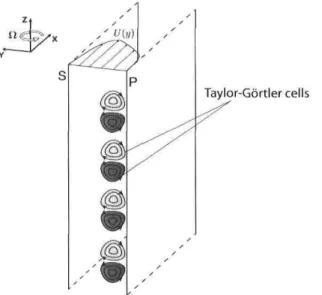
Since the expérimental data on turbulent flows in rotating référence frames is quite limited, an ambitious setup has been designed and built in the Expérimental Fluid Mechanics Laboratory at Laval University. This unique rig ( F I G . 1.1 ) consists of a 5-meter long rotating rectangular duct of high aspect ratio (AR = 11) destined to provide a fully developed two-dimensional flow. The whole unit has been designed to achieve £1 = 4 revolutions/s. The use of a settling chamber at the entrance of the main channel was not considered a worthwhile option because of strong centrifugal forces and size restrictions. Instead, the main channel is preceded by two latéral feeding channels that merge after a 180° turn. The hypotesis behind such a design is that the secondary channels will contribute to "pre-develop" the flow in terms of its z-vorticity and turbulence.
Récent measurements (FIG. 1.2) hâve shown however that the main flow characteristics at the two most downstream measurements stations (some 80h and 135/i from the main channel inlet, h being the main channel half-width) differ from the DNS results obtained by Alvelius et al. (1999). In order to simulate a two-dimensional Poiseuille flow, the
(a)
(b)
1. Blower 2. Control valve 3. PVCtubing 4. Contraction and pipe 5. Rotating shaft 6. Flow connectors
7. Latéral channels' chambers 8. Latéral channels 9. 180° turns 10. Main channel 11. Support beam 12. Tripod 13. Pulley 14. Disk break 15. AC motor
16. Instruments rotating shelf 17. Control PC computer
Figure 1.1: Expérimental setup. (a): top view; (b): side view. From Maciel et al. (2003). authors performed an unsteady calculation on a 3D domain with periodic conditions in the streamwise and spanwise directions. Since in the expérimental setup the flow is bounded in the z-direction, it is suspected that complex three-dimensional end-wall effects may affect the flow development and its characteristics.
a ) 20 10 1 ' ' ' 1 ' û 'â . / ^ ^ Ro f é^° " Ro
f
il,''' = 0.055 = 0.11 = 0.22 I I I i i ' ' ' ' A f1
i 1 i i i i 1 b) 4 -1 -0.5 0 0.5 y/h y/hFigure 1.2: Expérimental results (Maciel et al., 2003). (a): Mean streamwise velocity profiles at ReT ^ 180. D,x/h = 80; A,x/h = 118; - - , DNS (Alvelius et al, 1999). (b): R.m.s.
Chapter 1. Introduction
1.2 Objectives
Based on the aforementioned concerns, the main objectives of the présent study can now be formulated:
• To provide numerical modeling data to better understand the discrepancies between
the expérimental and DNS results.
• To contribute to the identification and understanding of the physical mechanisms responsible for the rotation effects.
• To elaborate stratégies to promote flow development in the rotating duct.
1.3 Methodology
In order to satisfy the set goals, 2D and 3D RANS simulations of the flow develop-ment in the actual expéridevelop-mental setup hâve been performed. The domains considered in the présent work include only the last portion of the latéral channels, the bcnds, the merging area and the main channel. Also, to save computer resources, only the upper half section of the channel is modeled and a symmetry plane is applied to the bottom boundary. Commercial codes Gambit 2.1 and Fluent 6.1 are employed as mesh gener-ator and flow solver respectively. Turbulence closure is achieved with a RSM model in order to better account for the complex anisotropic effects of rotation on the turbulent structures.
Fully developed solutions of a 2D and 3D rotating channel, obtained through peri-odic boundary conditions in the streamwise direction, are produced as référence cases. Moreover, they contribute to better understand the end-wall effects for high aspect ratio rotating duct fiows. The intensity and dynamic conséquences of 3D end-wall structures are examined and the effect of the Reynolds number (Re = U^h/v) and the Rotation number (Ro = 2Qh/Ub) on such flows are also investigated.
Moreover, the flow development in a duct having uniform inlet conditions (mimicking the présence of a settling chamber) is modeled in order to validate the design hypothesis stating that by pre-developing the flow in the two latéral channel, the fully developed state would be reached faster. Finally, many geometrical modifications, aimed at pro-moting the flow development in the main channel, are numerically tested in both two-dimensional and three-two-dimensional cases. The feasibility of implementing such devices in the expérimental setup are also discussed.
Theoretical background
It is well known that the Coriolis force, associated with System rotation, plays a funda-mental rôle in the stabilization or destabilization of turbulent shear flows. In the following chapter, the governing équations for an incompressible fluid flow in a rotating référence frame are presented. The non-dimensional parameters governing such flows are identified and flow phenomena are discussed.
2.1 Governing équations
For an incompressible flow in a rotating référence frame subject to constant rotation, the continuity and Navier-Stokes équations can be expressed as:
V - u = 0, (2.1)
- ^ + u • Vu = - - V p - f i x ( f î x r ) - 2 n x u + zA72u. (2.2)
ot p
The second and third ter m on the right side of équation (2.2) are the centrifugal and Coriolis forces respectively. The centrifugal force can be expressed as the gradient of a scalar quantity,
Q x ( f i x r ) = - V ( ^ 2 r
where r' is the distance from the axis of rotation. Hence, by replacing the pressure with the so-called reduced pressure (pred = p — | Q2r '2) , the Navier-Stokes équation can be
Chapter 2. Theoretical background 5
rewritten in a more compact and non-dimensional form:
- ^ + u • Vu = - V pr e d + — V2u - R o ( f î x u ) . (2.3) ot Re
Prom équation (2.3), it is apparent that the non-dimensional parameters dictating the fluid flow in a rotating référence frame are the Reynolds number Re = U^h/u and the Rotation number Ro = 2Qh/Ub- Hère, Ub represents the bulk velocity and h is the half-width of the channel. A combination of the Reynolds and Rotation number allows to define a new parameter, the Ekman number E = 1/ (Re • Ro).
Since ail computed results in the présent study are obtained using a RANS approach (Reynolds Averaged Navier-Stokes), it is relevant to introduce the complète set of N-S équations in a rotating référence frame under this form:
dx dy dz dx Re \ dx2 dy2 dz2
d —;r d —— d
I
-^-W2 - —u'v' - —u'w' + RoQV, (2.4)
dx dy dz TT
dV dV dV dP 1 fd
2V d
2V d
2V
U— + V— + W + +
dx dy dz dy Re \ dx2 dy2 dz2 ^ d -u'v' - —v'2 - —v'w' + RoQU, (2.5) dx dy dz dW dW dW dP 1 (d'2W d2W d'2W+ V—— + W-— = —— + — —— + —— +
dx dy dz dz Re \ dx2 dy2 dz'2 d d d — UW——VW W . VZ-DJ dx dy dzIn équations (2.4) to (2.G), the variables in capital letters are averaged quantifies whereas the lowercase variables with the prime exponent represent the fluctuations around the mean values.
2.2 Flow phenomena in a rotating channel
The rotating plane channel corresponds to a rotating duct of infinité aspect ratio
(AR = oo). If one further restricts to 2D flow solutions in a plane channel, one has W = d/dz = d2/dz2 = 0. By looking at équations (2.4) and (2.5), it is apparent then
streamwise velocity U. Therefore, the only efFect of rotation is to generate a pressure gradient in the direction normal to the flow, équivalent to a hydrostatic pressure field:
dy = -2Ro U. (2.7)
However, when a flow transitions to a turbulent state, rotation plays a much more significant rôle on the flow dynamics. The reason is that, as it will be shown in the next chapter, the Coriolis term appears in the Reynolds stress transport équation.
SUCTION SIDE
PRESSURE SIDE
Figure 2.1: Rotating turbulent channel flow. - —, Streamwise velocity profile for Ro > 0; , streamwise velocity profile for Ro = 0.
Therefore, one can state that system rotation lias an indirect efFect on the momentum équations through the Reynolds stress tensor. In the schematic of F I G . 2.1, it can be seen that the Coriolis force has three distinct effects on a turbulent Poiseuille flow:
• To croate a pressure gradient in the direction normal to the flow.
• To separate the flow in two zones: a région where the intensity of turbulence is increased and a région where turbulence is damped.
• To cause an asymmetry in the streamwise velocity profile (U) and thus, in the shear stresses on the two walls.
The first phenomenon is also présent for the laminar case and it simply arises from the necessity to generate a force able to equilibrate the Coriolis force. It is essentially identical to the event that takes place in a bend where a radial pressure gradient must be created to balance the centrifugal force.
The séparation of the flow in two distinct régions cornes from an inviscid flow analy-sis (Bradshaw, 1969) stating that conditions leading to instability are locally satisfied when the absolute vorticity ( = —(dU/dy — 2f2) is négative somewhere in the flow. Tins criterion predicts stability near the suction side wall, where dU/dy < 0, for ail positive rotation rates (11 > 0). For strong rotation rates it is even possible to hâve
Chapter 2. Theoretical background 7
relaminarization of the flow (zéro turbulent intensity) along the low-pressure side. Near the pressure side wall the physics is more diverse since for moderate rotation rates (i.e.,
dlJ/dy > 2fi > 0) instabilities can grow, but when the background vorticity (2f2) is
greater than the transverse gradient of the mean velocity, turbulence is once again weakened. A simple manipulation of the stability criterion allows to détermine that the critical value of the Rotation number for which the high-pressure side also becomes stabilized is 0.5. The enhancement of the turbulent intensity has a profound effect on the shear stress (r = fidU/dy — pu'v') along the pressure side wall. Along this bound-ary, the wall shear stress is significantly increased due to the destabilizing effect of the Coriolis force.
As shown in FlG. 2.1, the mean streamwise velocity profile is no longer symmetric when the system has an angular rotation rate. The maximum of the streamwise velocity is shifted toward the suction side since the flow is subject to less "résistance" in this ré-gion. It is also observed that in a certain zone the slope of the mean velocity profile is close to the value of the background vorticity, but so far there is no clear explanation in the literature about this behaviour.
2.3 Flow phenomena in a rotating duct
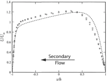
This section présents a discussion of the flow phenomena that occur when the channel is bounded by a lower and upper wall. From now on, a channel with a finite aspect ratio will be called a duct. The analysis will focus only on the upper end of the duct since a symmetry condition exists at the center plane of the domain. As shown in FlG. 2.2, the présence of a wall boundary in the xy plane and the subséquent no-slip condition causes a spanwise variation of the streamwise velocity profile. On the contrary, the transverse pressure gradient is essentially uniform in the spanwise direction. Therefore, near the upper wall boundary the axial velocity is reduced in magnitude and the Coriolis force (2f2 x U) is no longer sufficient to balance the pressure gradient. This results in the génération of a secondary flow driven in the positive y-direction by the pressure force. The secondary flow is associated with the génération of streamwise vorticity (ux). The
origin of such vorticity can be understood from the analysis of the laminar vorticity équation in a rotating référence frame:
Du) o
— = (w + 2fi) • Vu + vV2u>. (2.8)
Knowing that the rotation vector (Q) has only a spanwise component, the vorticity équation in the x-direction becomes:
DLJX dU dU . n . OU fd2uoT d2ux d2cux\ . .
+ + ( +
n) + v —f + ~ + -^ . (2.9)
If the analysis is limitée! to the région near the upper-wall boundary where the secondary flow is generated, équation (2.9) reduces to:
Dux „ dU
1)1,
o
oz
(2.10) Equation (2.10) states that the streamwise vorticity, also called the Ekman vorticity, is generated from a rotation of the background vorticity Unes which are aligned in the z-direction. The région where the secondary flow is generated is commonly named the
x U{
Figure 2.2: Secondary flow génération in a rotating duct.
Ekman layer. As it will be presented later on, the thickness of this layer is function of the Reynolds and Rotation numbers. In the next chapters it will be shown that, even for high aspect ratio ducts, the inomentum transport of the secondary flow has a major impact on the streamwise velocity profile at the symmetry plane of the duct. The présence of a secondary flow near the horizontal boundaries is possible even for very low Rotation numbers, but two new mechanisms appear only when the rotation rate increases. The ones discussed hère are the génération of longitudinal roll cells (Taylor-Gôrtler type vortices) and the instauration of the Taylor-Proudman-like régime in turbulent rotating duct flow.
Experimentally, the first observation of roll cells was made by Johnston et al. (1972) when they noticed large-scale streamwise structures near the pressure side wall of a rotating duct apparatus. The authors stated that the cell patterns seemed to be 'steady' in the sensé that the time period over which a pattern persisted was long relative to the turbulence time scales. However, no truly steady cell pattern was clearly identified. In the paper of Lezius & Johnston (1976), a two-layer model of a turbulent flow is employed to estimate the critical rotation number necessary for the onset of roll cells instabilities. Their study predicts that in fully turbulent flow (Re > 6000) the appearance of roll cells structures is essentially independent of the Reynolds number and begins to take place for a Rotation number Ro ~ 0.02.
Chapter 2. Theoretical background
As illustrated in F I G . 2.3, the roll cells instability appears under the form of counter-rotating longitudinal vortex pairs. Thèse vortical structures induce a velocity that, between the positive and négative members of each vortex pair, sweeps the fluid particles away froin the pressure side of the duct. On the contrary, between counter-rotating pairs they draw the flow toward the pressure wall. This transport has a noticeable effect on the streamwise velocity and turbulent activity across the duct. The DNS data of Kristoffersen & Andersson (1993) supports the fact that the number of vortex pairs in a given duct must be an integer N. By assuming that the vortices are circular and that they occupy half the cross-section, one can estimate the number of pairs in the duct as:
where H is the height of the duct (Le., H/2h = AR). However, the shape and size of the roll cells may vary for différent Reynolds and Rotations numbers. Generally, the number of vortex pairs tends to increase with Ro, and the wavelength (A) of a pair of roll cells approaches 2/i at high rotation rates (Ro ~ 0.2), as suggested in F I G . 2.3. The aspect ratio is another parameter affecting the preferred wavelength of the vortices and, in certain cases, may prevent their formation.
Taylor-Gôrtler cells
Figure 2.3: Roll cells instability in rotating duct flow. Light gray contours: u>x > 0; dark
gray: u>x < 0.
When the rotation rate of the duct is further increased (i.e., Ro > 0.5), it leads to a restabilization of the flow toward a Taylor-Proudman-like régime. The direct con-séquence is a decrease of the turbulent intensity near the pressure side wall and the disappearance of the roll cells. This phenomenon is predicted by the displaced particle analysis of Tritton (1992) which states that the flow is stabilized everywhere in the duct for high enough rotation rates (|5| = —2H/UJZ > 1). This analysis assumes an
will occur at lower rotation rates than those theoretically predicted.
The Taylor-Proudman-like régime is characterized by a région in the spanwise direction where the flow is two-dimensional (d/dz = 0). The complète dérivation of the Taylor-Proudman theorem can be found in Tritton (1988), and thus only the main features are discussed hère. The first hypothesis is that in équation (2.2) the Coriolis term is large compared to both inertia and viscous terms (Le., Ro 3> 1 and Ê « 1). The steady state équation of motion thus reduces to:
2 O x u = — V p . (2.12) P
Such flow is called geostrophic. An important characteristic of this type of flow is that the pressure gradient is normal to the flow direction and therefore the pressure is constant along a streamline. Another feature of a geostrophic flow can be found by applying the curl operator to équation (2.12)
V x ( 2 O x u ) = 0. (2.13) The expansion of the curl gives
n • v u - u • v n + u(v • n) - n ( v • u) = o. (2.14)
Since Q is a constant, the second and third terms are zéro and the last terni is also nul because of the continuity condition. If the axis of rotation is chosen in the z-direction, équation (2.14) becomesn|-a (2.15)
Hence, there is no variation of the velocity field in the spanwise direction and it cor-responds, by définition, to a two-dimensional flow. It is important to mention that the solution of a rotating duct in a Taylor-Proudman-like régime will not necessarily correspond to the theoretical 2D solution of a rotating channel since the secondary flow due to end effects may play an important rôle.2.4 Flow phenomena in a bend
The génération of a secondary flow in a bend is a well known subject and is treated in many textbooks. The topic is discussed hère since in the expérimental setup (Maciel et al, 2003), that we wish to model in the présent study, the main channel is preceded by two latéral feeding channels that merge after a 180° turn. As shown in FlG. 2.4, a pressure gradient is generated in the radial direction (normal to streamlines curvature) in order to counteract the centrifugal force. However, near the top wall, the no-slip
Chapter 2. Theoretical background I I
condition imposes a velocity gradient in the spanwise direction. The réduction of the streamwise velocity in this région directly affects the magnitude of the centrifugal force, which is now unable to balance the established radial pressure force. Consequently, a secondary fiow is generated. Its présence increases the dissipative losses in the duct since slow moving fluid is convected from the wall into the main fiow and, by continuity, high-energy fluid is rnoved toward the wall.
Dean cells
Figure 2.4: Détails of the expérimental setup configuration. Secondary fiow génération in a bend (Dean-type cells).
In the configuration of tins expérimental setup, two 180° bends are présent and one expects to find two counter-rotating vortices in the entrance région of the main duct, as sketched on FlG. 2.4. Moreover, when the rig is subjected to rotation, the centrifugal vortices should strongly interact with the Ekman vortex associated to the end wall and the Coriolis force.
Numerical method
The présent numerical study of turbulent flows in rotating ducts is based on the solu-tion of the Reynolds Averaged Navier-Stokes équasolu-tions in conjuncsolu-tion with a Reynolds Stress Model for turbulence closure.
The following chapter provides a brief justification for the choice of this particular method as well as a detailed characterisation of the turbulence model and wall treat-ment. The basic features of the commercial finite volume code Fluent v6.1.22 are also discussed.
3.1 Fluent: a finite volume solver
Fluent is a commercial finite volume (FV) solver that has been used at the LMFN
("Laboratoire de Mécanique des Fluides Numérique") over the past several years. The code has proven its accuracy and reliability in many problems varying from the unsteady flow around an oscillating wing to the flow around a passenger vehicle. Moreover, Fluent has the capability to analyze physical phenomenon involving turbulence, compressible effects, heat transfer and chemical reactions. As mentioned above, Fluent is a finite volume code that uses the intégral form of the conservation and transport équations to solve for ail quantities at the center of each control volume (CV). For a given variable (0), and assuming that the velocity field and fluid properties are known, this yields:
<j)u-ndA= 6T,pV(f)-ndA+ I q^dV, (3.1)
where T^ is the diffusion coefficient for (f> and q^ is a source term. Since convective and diffusive fluxes at the CV faces are also needed, an interpolating scheme must be
Chapter 3. Numerical method 13
used. Finite volume methods can be adapted to any type of grid and this makes them suitable for complex geometries. A disadvantage of FV methods, compared to finite différence schemes, is that they require three levels of approximation (interpolation, differentiation and intégration). This feature makes it difficult to develop higher than second order discretization schemes in 3D (Ferziger & Peric, 1992).
The solver version employed in the présent study is Fluent v6.1.22 and ail meshes are generated using Gambit v2.1.6.
3.2 RANS approach to turbulent flows
It is well known in the CFD community that the most accurate approach to turbulence simulation is to completely solve the Navier-Stokes équations without averaging or approximation. This approach is called direct numerical simulation (DNS). In a DNS computation, ail turbulent scales are captured and ail fiuid motions are resolved. This implies an unsteady calculation and a three-dimensional flow field. Moreover, a valid direct numerical simulation requires that each dimension of the domain must be at least a few times the scales of the largest turbulent eddies (L), and that the mesh discretization is fine enough to capture the smallest scales on which the viscosity is active (the Kolmogoroff length scale, rf). A quick estimation gives that the minimum number of cells required in each direction is L/rj. In their book, Tennekes and Lumley (1976) hâve shown that this ratio is proportional to i?e3//4. Since the time step is related
to the mesh size, the total cost of a DNS computation is proportional to Re3. With
the current computer performance, it is easy to comprehend why DNS is only used to solve simple flow geometries at low Reynolds numbers (Re ~ 103). Because the présent
numerical study involves an elaborate geometry and turbulent flows at Re > 104, the
DNS approach did not appear as a viable option.
A second approach to turbulent flows is large eddy simulation (LES). The fundamental principle behind this method is that the small scales are much weaker and provide little transport of conserved properties compared to the large scales. LES still remains a time dépendent three-dimensional computation but it requires a much smaller number of grid points since ail small eddies are now modeled, and only large eddies are simulated. This explains why LES is becoming increasingly popular among CFD users (mainly among scientists still today). However, large eddy simulations are often run on powerful cluster machines and, depending on the flow complexity, they still require days in terms of Computing time. As mentioned in the introduction, several geometries at various flows régimes hâve to be tested in the current study and the LES approach thus appears too demanding for the présent purposes.
time scales in the flow are regarded as part of turbulence and can thus be averaged. In a statistically steady flow, the velocity and pressure fields can be expressed as the sum of a time-averaged value and a time-varying fluctuation about that value:
u(x,t) = U(x) + u'(x,t),
p(x,t) = P(x) + p'(x,t).
If the flow is unsteady, time averaging cannot be applied and it is replaced by ensemble averaging. When this décomposition and averaging process is applied to the Navier-Stokes équations, it yields the Reynolds Averaged Navier-Navier-Stokes équations ((2.4) to (2.6)). It is easily verified that the number of unknowns is greater than the number of équations. In order to hâve a closed set of équations, it is necessary to introduce a turbulence model. Many models hâve been developed over the years and they can be divided in two catégories: eddy-viscosity models and Reynolds stress models. The former are based on the Boussinesq hypothesis stating that the Reynolds stresses can be approximated as follows:
dUA 2
where k is the turbulent kinetic energy:
With this type of turbulence modeling, the RANS équations hâve the same form as the Navier-Stokes équations except that the molecular viscosity is now replaced with an
effective viscosity //e// = I1 + l^t- Many models hâve been developed in order to
evalu-ate the eddy viscosity (/it) but the most popular are k — e, k—u, and Spalart-Allmaras
models. The great advantage of the eddy viscosity models is that they are easy to implement in a computer code and they perform relatively well when the hypothesis of local equilibrium is respected (e.g., zéro pressure gradients boundary layers). However, in many cases, this assumption is not valid and such models cannot be employed accu-rately.
The second and more elaborate approach to RANS turbulence modeling is a second order closure scheme. This method gives a more complète description of the energy exchange between the mean flow and the turbulence. Moreover, it has the great advan-tage of taking into account the anisotropy of turbulence. The Reynolds Stress Model (RSM) belongs to this category and its transport équations can be derived from the
Chapter 3. Numerical method 15
Navier-Stokes équations (2.2) as follows (from Mârtensson, 2004):
dxk J p \ dxj dxi
+ ~ [ v^r
1) - / - Uu'
3u'
k+
P- (u&k + u'jS
ik) (3.3)
dxk \ dxk dxk \ J p J du'j dxk uiUmejkm) : where Cij = Convection Pjj = Production <î>jj = Pressure strain Djj = Molecular diffusion Tjj = Turbulent diffusion £ij = Dissipation
Rij = Redistribution due to the Coriolis force.
Of the numerous terms of équation (3.3), CV,, P{j D^ and -Rjj can be solved directly. However, Tij, $jj and e^ need to be modeled in terms of computed quantities in order to hâve a closed set of équations.
The turbulent diffusion term is approximated with the generalized gradient-diffusion modelof Shir (1973):
dx
kya
ke dx
kJ
where C^ = 0.09 and ok = 0.82.
Fluent vô.1.22 offers an optional SSG model proposed by Speziale, Sarkar and Gatski
(1991) in order to calculate the pressure-strain term. This approach is a variant of the standard linear pressure-strain model (Gibson and Launder, 1975) and it has demon-strated to provide superior accuracy for rotating shear flows and complex engineering flows where streamline curvature is présent. The SSG model, also called the quadratic
pressure-strain model (QPS), is defined as follows: C{P) bij + C2e( blkbkj -(3.5) ( 2 \ +C4 k bikSjk + bjkSik - -bmnSmn5ij ) +C5k {bikujjk + bjkujlk) V 6 J where P = \Pk 2k 1 l du^ _ 9i
and the constants are (from Fluent 6.1 documentation):
Ci = 3.4; C{ = 1.8; C2 = 4.2; C3 = 0.8; Q = 1.3; C4 = 1.25; C5 = 0.4.
Assuming the isotropy of the dissipative structures, which is plausible far from the solid boundaries at high Reynolds number, the dissipation rate can be modeled as:
el3 = \e5l3. (3.6)
à
The scalar dissipation e is computed from a transport équation,
* a* a " ,
+^ M
+\c^-c" (3.7)
where ae = 1.0; CeX = 1.44; Ce2 = 1.92.
As for ail differential équations, boundary conditions are required for each équations. This subject is discussed in the next section.
Chapter 3. Numerical method 17
3.3 Wall treatment
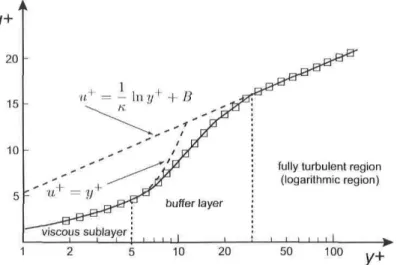
Turbulent flows are greatly affected by the présence of walls. Numerous experiments hâve shown that the near-wall région can be divided into three separate layers: the viscous sublayer, the buffer layer and the fully turbulent layer (see FlG. 3.1). Very close to the wall (Le., viscous sublayer), the molecular viscosity of the fiuid plays an important rôle in damping the velocity fluctuations. Further from the solid boundaries (i.e., fully turbulent région), the turbulence intensity increases rapidly due to the large velocity gradients. An accurate représentation of the near-wall région is critical to the
u+
10
fully turbulent région (logarithmic région)
10 20 50 100
y+
Figure 3.1: Velocity profile as a function of distance normal to the wall. D, Expérimental data; , wall functions. From Ferziger & Peric, 2002.
overall flow solution. In CFD, the conditions at solid boundaries can be treated in two separate ways. The fixst and more direct method is to solve the équations accurately up to the wall and apply the usual no-slip conditions for the velocity. For the Reynolds stresses and the dissipation, "low-Reynolds models" are often used in order to properly damp turbulence in the viscous sublayer. The setback with tins approach is that, at high Reynolds number, the viscous sublayer becomes very thin and many grid cells are necessary in order to well résolve it. The alternative is to use a wall function. Tins approach relies on the existence of an expected logarithmic région in the velocity profile such that:
u = U/uT = -lny+ + B, (3.8)
where K is the von Karman constant (K = 0.41), B is an empirical constant (B~ 5.45) and y+ is the normalized wall distance:
In équation (3.9), uT is the friction velocity (uT = \frw/'p) and y is the normal distance
to the nearest wall. The standard wall function in Fluent is based on the proposai of
Computation node
Wall function région
vt
«
40Figure 3.2: Wall function approach.
Launder and Spalding (1974) and is ernployed whenever the first cell has a yfc > 11.225.
From équation (3.8), and assuming that the flow is in local equilibrium (i.e., produc-tion and dissipaproduc-tion of turbulence are equal), one can show that uT = Cj \fk. The
expression for the rnean velocity at the first grid point can thus be written as:
= u+uT = In y+ + B\ ClJAkl'\ (3.10)
where Cfl = 0.09. The production of turbulent kinetic energy (k) in the wall région is
computed frorn:
OU £<V4fcl/2
Pk ~ Tw —- = Tw -ï . (3.11)
on K yfc
The dissipation at the wall-adjacent cells is obtained assuming, once again, local equi-librium:
e =
Cji
/4
fc
3/
2« 2/fc
(3-12) Finally, the near-wall values of the Reynolds stresses are derived from the wall functions:
u = 0.655, u'2 - ^ = 1.098, k 'ii,
u'?
-2- = 0.247, ^ k k = 0.255, (3.13)where, in a local coordinate System, the index r représenta the tangential coordinate,
r\ the normal coordinate and A the binormal one. To evaluate the turbulent kinetic
energy at the wall-adjacent cells, the k transport équation must be solved:
dk i/t\ dk\ 1
ok) dxjj 2
(3.14) where o^ ~ 0.82. Even though the values of k are only needed in the cells contiguous to the wall, équation (3.14) is solved in the entire domain for computational convenience. It is relevant to mention that the standard wall function is valid when the .first grid
Chapter 3. Numerical method 19
point is situated in the logarithmic région (Le., y^c > 30). However, the optimal range
is comprised between yfc = 30 and 60 (FlG. 3.2). In problems where the equilibrium
hypothesis is not valid (e.g., separated flows), the standard wall functions become less reliable and the user should verify that such flow régions do not exist over a large portion of the domain. In the case of rotating duct flows, the Coriolis force can cause the velocity profile to départ from the standard logarithmic behavior, especially near the suction wall. The validity of using a wall function approach in rotating flows is discussed in section 4.1.
3.4 Numerical schemes
Ail numerical results are obtained with a segregated type solver where the govern-ing équations (continuity, momentum and turbulent quantities) are solved sequentially within a given loop. Since the governing équations are non-linear and coupled, many itérations of the solution loop must be performed before a converged solution is ob-tained. In addition, the non-linear équations hâve to be linearized. The linearization method is "implicit" due to the fact that, for a given variable, the unknown value in each cell is computed using a relation that implies both existing and unknown values from neighbouring cells. This results in a System of linear équations with one équation for each cell in the domain. Fluent employs an itérative Gauss-Seidel linear équations solver in conjunction with an algebraic multigrid (AMG) method to solve for the dé-pendent variable in the System of équations. In the following section, the main features of the discretization schemes are addressed since they hâve a signifîcant impact on the accuracy of the solution.
In order to reduce numerical diffusion and achieve a higher degree of précision, a second order upwind scheme is chosen. In Fluent, this scheme uses a multidimensional linear reconstruction approach where the values at the cell face (see FlG. 3.3) are obtained through a Taylor séries expansion of the cell-centered solution about the cell centroid:
cf)e = (j)P + V 0 P • A s (3.15)
where As is the displacement vector from the upstream cell centroid (P) to the face centroid (e), and the gradient V0 is computed using the Green-Gauss theorem. In ail simulations performed hère, the second order scheme is selected for momentum, turbulent kinetic energy, turbulent dissipation rate and Reynolds stress équations. Diffusion terms are always discretized using a central différence scheme that provides second order accuracy.
The remaining variable to be calculated is the pressure. Since the momentum équations are already employed to détermine the velocity components, the only équation allowing
to solve for pressure is the continuity condition. Unfortunately, for incompressible nows the latter does not contain any pressure terni and therefore some manipulations are required. The most common method is to take the divergence of the momentum équation and to apply the continuity condition in order to simplify certain ternis. The resuit is a Poisson équation for pressure:
d dp_ dx.i
d
dx, (3.16)
Equation (3.16) is coupled with the momentum équation and is solved using the PRE-STO! scheme (pressure staggering option). This particular model is recommended for rotating fiows and flows in strongly curved domains. Since both of thèse conditions are met in the présent study, the PRESTO! model is the preferred pressure interpolation scheme. w n ne w #p sw s se NE EE Ay
Figure 3.3: Finite volume approach for a Cartesian 2D grid. From Ferziger & Peric, 1992. In order to guarantee that the pressure and velocity fields satisfy the momentum and continuity équations, a "correction method" has to be used. With this approach, the ve-locity and pressure fields computed from the linearized momentum équations are taken as provisional and a correction is applied to them in order to enforce the conservation law. When this procédure is applied to équation (3.16), it yields a pressure-correction équation. Many options are available for solving this latter équation, but the approach chosen hère is the SIMPLEC algorithm (van Doormal and Raithby, 1984).
Chapter 4
Validation efforts
Before modeling the expérimental setup, many numerical tests are performed on much simpler configurations in order to validate the CFD code for flows in rotating channels. The présent investigation will demonstrate the ability of the RSM model, and its wall function, to capture the effects of rotation on turbulence. The soundness of the bound-ary conditions and their ability to mimic the expérimental conditions are also asserted.
4.1 Validation of the turbulence model and wall
treatment
As it was stated in the previous chapter, the second order closure schemes are expected to be a more accurate approach to turbulence modeling than the simpler and cheaper first order counterparts. The great advantage of using a Reynolds Stress Model (RSM) is that the rotation effects are implicit in the model without any adjustment or correc-tion.
The présent validation of the Reynolds Stress Model is done by running a simulation of a fully developed turbulent flow in a non-rotating and rotating channel, and by comparing the results with the DNS calculations of Alvelius et al. (1999). Moreover, two meshes of différent size are used in order to assert the mesh independence of the solution. The coarse grid has 80 éléments in the streamwise direction (x-direction) and 35 in the transverse direction (y-direction), uniformely distributed (see F I G . 4.1). The refined grid has the same discretization in the streamwise direction and 51 cells in the transverse direction. Since a wall function is employed in the near-wall région, the size of the wall-adjacent cell is set to y^c ~ 40 which does not correspond to the
saine physical size on each side of the rotating channel. The domain has a length of lO/i and a width of 2h, where h is the half-width of the channel. Periodic conditions are applied at the inlet and outlet boundaries while a prescribed flowrate is imposed in the x-direction. The domain length and streamwise discretization are chosen in order to guarantee a d/dx = 0 (fully developed condition) along the channel. One should
SUCTION SIDE WALL
IJflffjï
1 mm
' \ ' ftfR I
BilIlIlnilBMflt
1
• • • • • •
r' 11 i m 1 î ut 1 m
i-H
1 r H H H F -I ml H m 1 In F m
PRESSURE SIDE WALL
Figure 4.1: Coarse mesh for rotating case.
note that the periodic conditions only irnply that the solution at the two boundaries raust be identical, and therefore, an évolution along the domain is allowed. However, it is reasonable to expect a uniform solution in the streamwise direction under such conditions. Further information about this issue is presented in Appendix A.
TABLE 1.1 and 4.2 compare the predicted ReT = uTh/v values on the suction and
pres-sure side walls of the channel. This paranieter represents a ratio between the turbulent
RANS (coarse mesh) RANS (fine mesh) DNS (Alvelius) Re 351 351 358 s r .5 .9 .7 Re* 351.5 351.9 359.3 Re, 351. 351. 359. 5 9 0 Table 4.1: Comparaison of non-rotating case - Re = 6210.
and viscous transport and allows to evaluate the validity of the turbulence modeling in the near-wall région. The values of ReT listed in TABLE 4.1 as well as the profiles
plotted in F I G . 4.3a indicate that, without System rotation, the solution is symmet-ric and the RANS modeling is able to capture relatively well the near-wall behaviour (about 2% on ReT). Prédictions are particularly good for the u'v' stress component,
RANS (coarse mesh) RANS (fine mesh) DNS (Alvelius) ResT 306.1 305.8 279.9 Re'^ 415.2 416.2 426.6 ReT 360.7 361.0 353.3
Chapter 4. Validation efforts 23
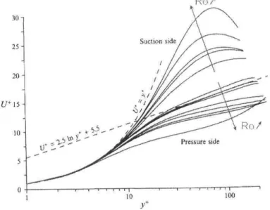
which is the only non-vanishing Reynolds stress term in the x-momentum équation. When System rotation is présent, the symmetry is broken and the velocity profile shows a central région of near constant slope (dU/dy = 2Q). The RANS prédictions match fairly well with the DNS results of Alvelius et al. (1999) even though the estimâtes on the suction (stabilized) side are less accurate. Thèse results are not surprising since turbulence is damped in tins portion of the channel and there is a déviation frorn the standard log-like behaviour. The computations of Kristoffersen & Andersson (1993) il-lustrate this phenomenon ( F I G . 4.2). It is interesting to notice that for high Rotation
Ro/
3 0 1
100
Figure 4.2: Mean velocity profiles in wall coordinates for différent rotation rates (0 < Ro < 0.50) at Re = 2900. Prom Kristoffersen & Andersson, 1993.
numbers, the mean velocity profile near the suction side has a more laminar-like shape and approaches the linear law u+ = y+. Normally, for such low Reynolds number flows,
the wall function approach would not be necessary but, for the moment, Fluent does not offer an efficient wall damping model.
In the présent study, the Reynolds number will vary between 10000 and 40000 and it is expected that the wall function will perform better since the existence of a logarithmic région in the velocity profile is formally verified for an infinité Reynolds number.
b)
o"
Figure 4.3: Normalized mean velocity profiles and Reynolds stress components. D, Coarse mesh; A, fine mesh; - —, DNS by Alvelius. (a): Re = 6210 at Ro = 0; (b): Re = 6899 at Ro = 0.20.
Chapter 4. Validation efforts 25
4.2 Validation of the boundary conditions
In the finite volume method, each CV provides an algebraic équation but the fluxes through the faces located along the domain boundaries require a spécial treatment. Those fluxes must be known or hâve to be a combination of interior values and bound-ary data. Fluent offers a variety of boundbound-ary conditions for both the inlet and exit boundaries, but only a few are mentioned hère below:
• Inlet conditions: velocity inlet, pressure inlet, mass flow inlet
- Velocity inlet: allows to define the flow velocity, along with ail relevant
scalar properties of the flow. The total (or stagnation) properties of the flow are not fixed, so they will rise to whatever value is necessary to provide the prescribed velocity distribution.
- Pressure inlet: allows to define the fluid total pressure at flow inlets, along with ail other scalar properties of the flow. They are suitable for both in-compressible and in-compressible flow calculations and can be used even if the flow rate and/or velocity is not known.
- Mass flow inlet: provides a prescribed mass flow rate or mass flux dis-tribution at an inlet. It is often used when it is more important to match a prescribed mass flow rate than to match the total pressure of the inflow stream.
• Exit conditions: outflow, pressure outlet
- Outflow: allows to model flow exits where the détails of the flow velocity and
pressure are not known prior to solution of the flow problem. No conditions are specified by the user at outflow boundaries but a zéro normal diffusion flux is assumed.
- Pressure outlet: requires the spécification of a uniform static pressure at the outlet boundary.
• Wall boundary conditions: used to separate fluid and solid régions. In viscous flows, the no-slip boundary condition is enforced by default, but a tangential velocity component in terms of the translational or rotational motion of the wall can also be specified.
• Symmetry conditions: useful when the physical geometry of interest and the flow patterns hâve mirror symmetry. This condition can also be used to model zéro
shear slip walls in viscous flows. A symmetry conditions assumes zéro convective and diffusion fluxes across the boundary.
• Periodic conditions: helpful when the physical geometry of interest and the flow patterns possess a periodically repeating nature. When a pressure drop or a fiowrate are specified across translational periodic boundaries, this condition en-ables to model fully developed flows.
Although many options are available, the preferred entrance condition for analyzing the flow development in a rotating duct is the velocity inlet since it allows to specify a given velocity and/or turbulent profile as inlet condition. Hence, the conditions présent in the expérimental setup can be reproduced in the computational domain. This b.c. is also very interesting for demanding problems since the domain can be separated in many smaller sub-domains and the flow solution at the exit of a section can be set as inlet condition for the following downstream section.
The choice of an exit condition is more délicate since it often assumes a certain flow state. For example, the pressure outlet condition présumes that the value of the static pressure is uniform on the boundary. This b.c. is certainly inappropriate for modeling the flow in a rotating duct, since it is well known that rotation, through the action of the Coriolis force, générâtes a pressure gradient in the direction normal to the flow. Consequently, the pressure along the outlet boundary is not uniform. A more suitable exit condition is the outflow because no restrictions are enforced on the pressure dis-tribution at the boundary. However, the outflow condition is formally respected only in fully developed flows. Since in the présent study, the flow at the exit boundary is rarely close to full development, it is necessary to verify the effect of such condition on the solution. For this purpose, the flow development in a rotating channel is chosen as the test case. Two rectangular domains of width 2h, but having différent lengths are considered (60/i and 100/i respectively). The same boundary conditions are applied to both domains (Le., a uniform velocity profile with no turbulence at the entrance, an
outflow condition at the exit and solid walls on the sides of the channel). The mesh
discretization in the transverse direction is identical for both cases. In the streamwise direction, the channel having a length of lOO/i has the same discretization as the shorter channel up to a distance of 60/i from the inlet. The remaining length of 40/i has a uni-form mesh and "grid continuity" is respected.
In the following analysis, the flow development in each domain is compared at two posi-tions along the channel. The first station is at a distance x/h = 50. The second position coincides with the exit boundary of the short domain (x/h = 60). The long domain will serve as the référence case since the outflow b.c. is very far from the measurement stations and it is thus reasonable to assume that it has no effect on the flow solution at the two given stations.
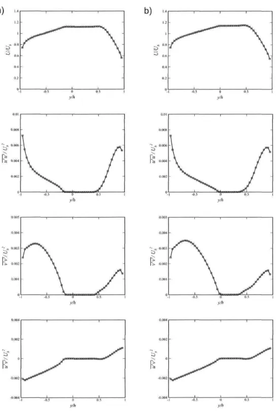
Chapter 4. Validation efforts 27
T> 0.002
-Figure 4.4: Normalized mean velocity profiles and Reynolds stress components at Re = 40000 and Ro — 0.22. • , Domain of length 60h; , domain of length 100/t. (a): Measurement station at x/h = 50 (lO/i from exit boundary of shorter domain); (b): measurement station at x/h = 60 (at exit boundary of shorter domain).