Properties of a diffuse interface model based on a porous medium theory for solid–liquid dissolution problems

This is an author-deposited version published in :

http://oatao.univ-toulouse.fr/

Eprints ID : 8799

To link to this article : DOI:10.1007/s10596-012-9295-1

URL :

http://dx.doi.org/10.1007/s10596-012-9295-1

OATAO is an open access repository that collects the work of Toulouse researchers and

makes it freely available over the web where possible.

To cite this version :

Luo, Haishan and Quintard, Michel and Debenest, Gérald

and

Laouafa, Farid

Properties of a diffuse interface model based on a

porous medium theory for solid

–liquid dissolution problems

.

(2012) Computational Geosciences, vol. 16 (n° 4). pp. 913-

932.

ISSN 1420-0597

Any correspondence concerning this service should be sent to the repository

administrator:

[email protected]

Properties of a diffuse interface model based on a porous

medium theory for solid–liquid dissolution problems

Haishan Luo · Michel Quintard · Gérald Debenest · Farid Laouafa

Abstract In this paper, a local non-equilibrium diffuse

interface model is introduced for describing solid– liquid dissolution problems. The model is developed based on the analysis of Golfier et al. (J Fluid Mech 457:213–254, 2002) upon the dissolution of a porous domain, with the additional requirement that density variations with the mass fraction are taken into account. The control equations are generated by the upscaling of the balance equations for a solid–liquid dissolution using a volume averaging theory. This results into a dif fuse interface model(DIM) that does not require an explicit treatment of the dissolving interface, e.g., the use of arbitrary Lagrangian–Eulerian (ALE) methods, for instance. Test cases were performed to study the features and influences of the effective coefficients in-side the DIM. In particular, an optimum expression for the solid–liquid exchange coefficient is obtained from a comparison with the referenced solution by ALE

H. Luo (

B

Allée Camille Soula, 31400 Toulouse, France e-mail: [email protected] M. Quintard e-mail: [email protected] G. Debenest e-mail: [email protected] H. Luo · M. Quintard

CNRS, IMFT, 31400 Toulouse, France H. Luo · F. Laouafa

Institut National de l’Environnement Industriel et des Risques, Parc techncologique ALATA BP2, 60550 Verneuil-en-Halatte, France

e-mail: [email protected]

simulations. Finally, a Ra–Pe diagram illustrates the interaction of natural convection and forced convection in the dissolution problem.

Keywords Diffuse interface model ·

Porous medium theory · Numerical simulation

Mathematics Subject Classifications (2010) 76V05 ·

76S05

Nomenclature

Aβσ Surface between the β-phase and the σ -phase (square meters)

DAβ Molecular mass diffusion coefficient (square

meters per second)

g Gravity (meters per square second) K Permeability (square meters)

Kβσ Mass exchange between the β-phase and the σ-phase

nβσ Normal vector to the β–σ surface p Pressure (pascal)

P Averaged pressure (pascal) V Volume (cubic meters)

vβ β-Phase velocity (meters per second) vσ σ-Phase velocity (meters per second)

vAβ Velocity of species A in the β-phase (meters

per second)

v_Bβ Velocity of species B in the β-phase (meters per second)

Vβ β-Phase averaged velocity (meters per second) w Interface recession velocity (meters per

second)

εβ β-Phase volume fraction

ρ Density (kilograms per cubic meter) ˜

µ Chemical potential (joules per mole) µ Dynamic viscosity (pascal second) ωAβ Mass fraction of species A in the β-phase

ÄAβ Averaged mass fraction of species A in the

β-phase

1 Introduction

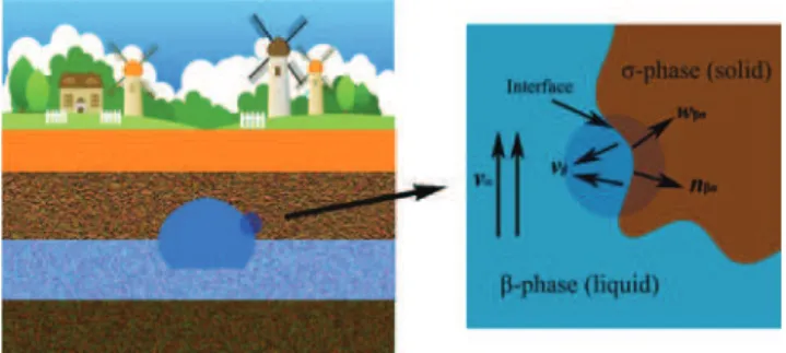
Dissolution of solid matter or porous media is a typ-ical problem widely encountered in many industrial fields, for instance, to mention a few applications, al-loy melting, corrosion of carbonate rocks, acid injec-tion into petroleum reservoirs, ablainjec-tion of composite layers in rocket nozzles, etc... In the case concerned by this paper, dissolution of soluble rocks, e.g., salt mines, may lead to the expansion and collapse of the underground cavity, as illustrated in Fig.1, which is a potential environmental risk. Numerical modeling of the evolving cavity is a method of choice for any safety analysis. Several numerical works were concerned by the dissolution of porous media, such as those done by [15, 52, 53]. While the model studied in this paper is directly linked to these approaches and, therefore, can handle true fluid/porous media dissolution problems, we are interested in applications for which the flow in the “solid” domain is close to zero, either because of very slow permeability or because the permeability it-self is zero. In these situations, the solid and liquid bulks are connected directly by an interface at any scales, which, in principle, may preclude the direct utilization of porous media models. Instead, it should be regarded as a type of moving interface problem, and many direct techniques have been designed to handle such cases, such as the arbitrary Lagrangian–Eulerian (ALE) tech-nique used as a “reference” in this paper. However, we show in our work, on the basis of a quantitative compar-ison with “reference” computations, that porous media

Fig. 1 Solid–liquid dissolution caused by groundwater

local non-equilibrium theories can indeed be used to deal with such problems.

For sake of simplicity, we consider the case of a binary system, i.e., the chemical solute constituting the solid is dissolved by a “solvent” (mainly water in most practical applications). Dissolution is controlled in this case by thermodynamic equilibrium at the interface, i.e., equality of the chemical potentials. This equality translates, for such a two-component system, into a simple Dirichlet condition for the concentration at the solid–liquid interface. An alternative choice for the boundary condition is to apply a reactive model, i.e., the mass flux between solid and fluid at the interface is determined by a reaction term. In most practical cases, e.g., salt mines, the reaction rate is very fast so that the reactive model approaches to the former boundary model, or the dissolution model based on equilibrium conditions is correct. Without loss of generality, we only consider very fast chemical reactions in this paper, or purely thermodynamic equilibrium problems. When applying this boundary condition to the mass transport equations that control the dissolution process, the so-lution of these PDEs will lead to a recession of the interface.

From a numerical point of view, there are two classes of approaches to characterize the moving interface: sharp interface methods and diffuse interface meth-ods. Sharp interface methods can be further divided into two categories: front tracking and front capturing. Several front-tracking methods utilize a fixed grid with moving marker particles to track the fronts, such as [13,23,35,39]. Some front tracking methods adopt a separate grid, for example, the famous ALE method handles the computation in both an absolute frame and a relative frame, the movement of the mesh being taken explicitly in the Eulerian frame [12, 22]. Also, various explicit treatments of the interface movement have been developed in the framework of finite dis-cretization, e.g., finite volume formulation [44], random walk methods [4], etc... Recently, [51] developed an in-terface marker reconstruction method combined with a hybrid lattice-Boltzmann/finite-difference scheme [17]. These works have shown impressive simulation results. However, the major drawback of direct front track-ing is the complexity. Special care has to be taken to topological changes, e.g., the algorithm of the re-distribution of the interface markers is complicated. Further, the methods may have a poor behavior in the case of non-differentiable surfaces, for example, sharp angles. Compared to the explicit expression of the interface in the front-tracking methods, the interface is regarded implicitly in the front-capturing methods. The two most popular front-capturing methods are

volume of fluid (VOF) [16, 30] and level set [26, 34]. VOF method uses a color function to represent the phase volume fraction, which is subject to numerical diffusion. Therefore, reconstruction of the interface must be implemented. VOF methods have been asso-ciated with reconstruction algorithms that can handle streaks or peaks in interfacial gridblocks (development of specific piecewise linear interface calculation method like in [20]). For the level-set method, the interface is generally represented by the zero contour of a signed distance function (level-set function). The movement of the interface is governed by an advective equation for the level-set function, which is also affected by numerical diffusion. A reinitialization process is re-quired in order to maintain the level-set function as a signed distance function. However, level-set method is often reported as nonconservative. To overcome this weakness, [24] proposed to use a Heaviside function to take the place of signed distance function as a level-set function. Better conservation is observed by this im-provement. In fact, one can already find an initial trace of diffuse interface methods inside the VOF and recent level-set methods, as they have utilized the concept of phase field. However, the two methods still belong to sharp-front methods because the reconstruction or reinitialization of the interface can not be avoided. As the other big class of moving interface methods, the diffuse interface methods (DIM) consider the interface to be a diffuse layer where some quantities (especially a scalar field that plays the role of the phase indi-cator) vary rapidly but continuously [1, 3, 5, 19, 50]. This kind of opinion can be even dated up to two centuries ago, when Van der Waals [43] proposed that the physical interface should be continuous as a result of surface tension. The advantage of DIM compared to the sharp-front methods is that it does not need any special operation upon the interface during the compu-tation. Global control equations can be applied to the whole domain without phase distinctions, thus greatly improving the facility of coding and computation. In the past three decades, the DIM has been extensively developed for many moving-interface problems, e.g., flows in near-critical fluids [25], capillary waves [40], moving contact lines [33], droplet and nucleation [9], dendritic growth and solidification [8,32,45], adsorp-tion/desorption of material [37], metal alloys melting [18,38], micro-scale solute precipitation and dissolution [42,49], to list a few. These DIM works are generally based on the Cahn–Hilliard model [7], which is based on a free energy involving second gradient terms to “diffuse” the interfaces. Using real fluid characteristic leads to a physical interface, which is very thin in the case of solid–liquid dissolution. Very huge grid

num-bers are thus required to capture the narrow interface. In addition, the Cahn–Hilliard model contains fourth-order derivatives, which requires high-fourth-order numerical schemes. Adaptive mesh refinement is often applied to resolve around the interface to avoid the intolerable resource consuming, such as shown in [37]. Anyhow, the corresponding computations are often limited to a very small spatial scale, which could not meet the need for larger-scale simulations, such as those discussed in this paper. In addition, Cahn–Hilliard models in the case of multi-component problems pose several formu-lation problems with strong density variations, which are difficult to overcome. These difficulties motivated our study based on a completely different approach.

We take notice of the work of [15], who used a Darcy-scale local non-equilibrium model to study the dissolution regimes and wormhole development of porous media under different Pe and Da numbers (there is also a reminiscence of a local non-equilibrium theory in the case of solidification involving mushy zones [6, 31]). It is found that the porosity front becomes sharp when the mass exchange coefficient (which also can be understood as a Darcy-scale reaction rate that should not be confused with the pore-scale reaction rate) becomes large. The dissolution zone (if hydrodynamically stable) reaches rapidly a steady-state thickness, which may be controlled through the model parameters, in particular the mass exchange coefficient. In the limit of infinite mass exchange coefficient (in numerical practice: large enough), one recovers the local equilibrium dissolution front, i.e., a liquid–solid interface. This phenomenon is also observed by [51–

53]. In particular, they all found that the dissolution front can become unstable under certain conditions, e.g., large Da numbers [15,51], or based on the critical Zhao number proposed in [52,53]. Regardless of these instability mechanisms, the main point of these various studies is that, with the increase of the mass exchange coefficient, the dissolution mechanism will be limited by the mass transport toward the interface region. That is to say, the front moving velocity will not depend on the mass exchange coefficient beyond a certain critical value. Mathematically speaking, a finite mass exchange coefficient will not lead to an extremely sharp porosity profile. How can we use such porous media theories for problems involving solid–liquid interfaces? In fact, we can consider the solid–liquid interface as a porous medium region where the porosity varies from 0 to 1. The mass exchange coefficient in the interface re-gion can be artificially increased in order to sharpen the interface, while there is no need for an infinite value as discussed before. We only need to find a critical value to maintain a sufficiently sharp diffuse

interface, compatible with the physics we want to re-produce (for instance compatible with the boundary layers developing near the dissolving interface, as will be discussed later). As a result, a moderate mesh size can be used without generating significant inaccuracy. Based on this discussion, we follow the work of [15], then develop a DIM for solid–liquid dissolution prob-lems. This model is obtained from a volume averaging technique. The resulting equations feature two mass balance equations for the liquid involving an effective diffusion coefficient, D∗_{, and a mass exchange term,} α, both terms being a function of the porosity, εβ. The momentum equation that approaches the initial physics is a Darcy–Brinkman equation, which degenerates to Stokes equations when in the free fluid and Darcy’s law, with a permeability K(εβ), when in the diffuse interface region. Mathematically speaking, the inter-face in this model tends to be infinitively thin when the α coefficient tends to infinity. The thickness of the interface increases when α decreases. Therefore, α may be adjusted to reproduce approximately the interface at the desired accuracy. A very large α must not be used to avoid numerical resolution problems associated to very thin interfaces. In this paper, the α, D∗_{, and} K are obtained by solving “closure problems” with a unit cell abstracted from a plane flow. Since no real porous medium is present, meaningful modifications could be made to optimize their expressions. Several choices will be discussed in this paper. In addition, the density variation is added in the current model not only because of mass conservation accuracy reasons but also because of the Rayleigh–Bénard effects aroused by gravity [21,47,48], which may have a great impact on the evolution of the dissolution interfaces.

A one-dimensional analytical solution giving the boundary velocity is obtained to verify the DIM by comparison with the one obtained from the original sharp interface model. We would like to mention here that an alternative approach to prove the coincide of the original model and the phase-field model is based on the utilization of asymptotic techniques [42]. Follow-ing this mathematical analysis, an upscaled model for crystal dissolution and precipitation was derived, which is quite similar to the one proposed in this paper[41]. The convergence analysis, though, does not include the effect of advection, which is an important part of the investigation presented in this paper. The DIM model properties and performances will be analyzed on a classical test case involving the dissolution of a plane-flow structure. Finally, we will use the validated model to understand the impact of density variations on a tube dissolution problem. Indeed, flow and geometry evolu-tions will be controlled by the competition between

ad-vection and diffusion (as measured by a Péclet number, Pe) and the possible effect of hydrodynamic instabili-ties (natural convection, depending on the value of a Rayleigh number, Ra). Our numerical results show that diverse configurations may be obtained: the appear-ance of a thin boundary layer when Pe increases and the appearance of hydrodynamic instabilities (salt fingers) at high Ra numbers. This latter aspect is particularly im-portant as it tends to complicate the geometric structure of the dissolving interface (dissymmetry, roughnesses, ...).

In the next section, the diffuse interface model is deduced with the help of a volume averaging theory. In the third section, several examples are implemented to study the influence of the chosen effective coefficients. Finally, to illustrate the potential of the proposed model, a series of computations allow to plot a Pe– Ra diagram showing the various flow and geometry patterns obtained under different conditions.

2 Dissolution model

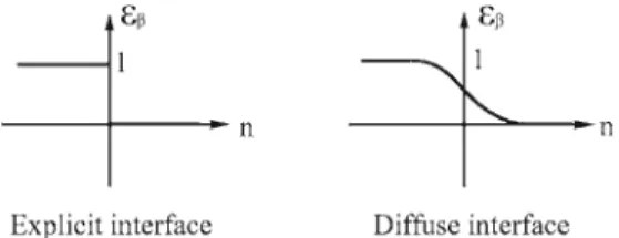
Figure1illustrates the exact interface for a solid–liquid dissolution problem. In the case of the binary system under investigation, the species concentration equals to an equilibrium value at the interface. We introduce a phase indicator, εβ, that has a unit value in the liquid and zero in the solid in the original dissolution model, as shown in Fig.2. Alternatively, for a diffuse interface method, the sudden jump of the variables will be replaced by a continuous distribution. A diffuse interface model may be obtained from different points of view, for instance on the basis of heuristic arguments. Because this brings some understanding on the phys-ical soundness of the model, we adopt here the idea that this model is an application of porous media non-equilibrium theories. In this paper, the DIM equations are developed from the original dissolution model using a volume averaging theory [46], taking into account the density variations with concentration. In Section 2.1, the original dissolution model is introduced. In Section

2.2, we present the upscaling method leading to the DIM equations.

2.1 Original multiphase model

Suppose the liquid phase β contains species A and B in a binary system and the solid phase σ contains only species A. We write the balance equations below.

The total mass balance equation for the β-phase is given by ∂ρβ ∂t + ∇ · ¡ ρβvβ ¢ = 0 (1)

The mass balance equations for species A and B in the β-phase are written as

∂¡ρβωAβ ¢ ∂t + ∇ · ¡ ρβωAβvAβ ¢ = 0 (2) ∂¡ρβωBβ ¢ ∂t + ∇ · ¡ ρβωBβvBβ ¢ = 0 (3)

where ωAβ, ωBβrepresent the mass fractions of species

A and B, respectively.

The mass balance equation for the σ -phase is written as

∂ρσ

∂t + ∇ · (ρσvσ) = 0 (4)

Generally, the solid phase is immobile; thus, vσ= 0. Here we keep vσ during the development because this might be interesting for theoretical reasons, for instance to see the evolution of the dissolving surface in a frame moving with the average dissolution velocity such as in [44].

The Navier–Stokes equations for the β-phase are written as ∂¡ρβvβ ¢ ∂t + ∇ · ¡ ρβvβvβ ¢ = −¡∇pβ− ρβg ¢ + µβ∇2vβ (5)

At the β–σ interface (denoted by Aβσ in the fol-lowing text), the chemical potentials for each species should be equal between the different phases. There-fore, for the special binary case under investigation, we have the following relations:

˜ µAβ ¡ ωAβ,p, T ¢ = ˜µAσ(ωAσ,p, T) at Aβσ (6) where ωAσ equals 1. It must be emphasized that in the

complete binary case, i.e., when ωAσ 6= 1, there is also a

relation similar to Eq.6for the other component. This results in a classical equilibrium condition imposing an equilibrium concentration for species A, i.e.,

ωAβ = ωeq at Aβσ (7)

The no-slip boundary condition at the β–σ interface gives:

vβ−nβσnβσ · vβ = 0 at Aβσ (8) The mass balances for species A and B at the β–σ interface give: ρβωAβ ¡ v_Aβ− w¢·nβσ = ρσωAσ(vAσ− w) ·nβσ at Aβσ (9) ρβωBβ ¡ vBβ− w ¢ ·nβσ = ρσωBσ(vBσ − w) ·nβσ at Aβσ (10) and the total mass balance at the β–σ interface gives: ρβ

¡ vβ− w

¢

·nβσ = ρσ(vσ− w) ·nβσ at Aβσ (11) where w represents the velocity of the interface and vσ = vAσ. As ωBσ = 0, the RHS term of Eq. 10

equals 0.

Equations9and11allow us to write the relation ρβωAβ ¡ vAβ− w ¢ ·nβσ = ρβ ¡ vβ− w ¢ ·nβσ at Aβσ (12)

Using a theory of diffusion [36], we have

ρβωAβvAβ= ρβωAβvβ− ρβDAβ∇ωAβ (13)

and the left-hand side of Eq.12may be written as

nβσ· ρβωAβ ¡ v_Aβ− w¢ =nβσ· ¡ ρβωAβ ¡ vβ− w ¢ − ρβDAβ∇ωAβ ¢ at Aβσ (14) and Eq.2can also be transformed as

∂¡ρβωAβ ¢ ∂t + ∇ · ¡ ρβωAβvβ ¢ = ∇ ·¡ρβDAβ∇ωAβ ¢ (15) The whole balance equations presented above are sufficient to solve the physical problem, provided that the overall surrounding boundary conditions are also given. One substitutes Eq.14 into Eq.9 and with the help of Eq.11, having

nβσ· w =nβσ · Ã vσ+ ρβ ρσ ¡ 1− ωAβ ¢ DAβ∇ωAβ ! at Aβσ (16) and nβσ· vβ=nβσ· Ã vσ+ ρβ− ρσ ρσ ¡ 1− ωAβ ¢ DAβ∇ωAβ ! at Aβσ (17)

It is emphasized here that for a tracer case (ωAβ≪ 1),

we recover the classical formation adopted by [15]. In summary, the above expressions give the reces-sion velocity and the β-phase velocity at the interface, which are necessary to implement the direct explicit numerical methods, for instance, ALE.

2.2 Diffuse interface model based on a porous medium theory

Contrary to explicit methods who consider the interface as a discontinuous surface, a diffuse interface method regards the interface as a transition layer where the quantities vary rapidly but smoothly. The whole do-main is considered to be a continuous medium without the direct distinction of solid or liquid, etc... Golfier et al. [15] studied one example of a local non-equilibrium dissolution model for porous media. It has the ability to be very close, with a proper choice of the exchange term (α) to the local equilibrium solution, which is equiva-lent to the original dissolution problems. Therefore, it is a good candidate for a diffuse interface model. We develop, in the section below, this model for dissolu-tion including the effect of density variadissolu-tion. In our studied case, the σ -phase is immobile, i.e., vσ = 0 in the following analysis. The volume averaging theory [15, 27, 29, 46] will be used to upscale the balance equations.

According to the volume averaging theory, the aver-aged form of Eq.2can be expressed as

∂­ρβωAβ ® ∂t + ∇ · ­ ρβωAβvAβ ® = −1 V Z Aβσ nβσ · ρβωAβ ¡ vAβ− w¢ dA (18)

We define the average of the mass fraction as ÄAβ = ­ ωAβ ®β = ε−1β ­ ωAβ ® = 1 Vβ Z Vβ ωAβ(r)dV (19)

and the average of the velocity as

Vβ = ­ vβ ® = εβ ­ vβ ®β = 1 V Z Vβ vβ(r)dV (20)

where εβ is the volume fraction of the β-phase, Vβ is the filtration velocity and ­vβ

®β

is the phase intrinsic average velocity.

The mathematical deduction of the DIM is presented in AppendixA. Finally, we have the form of the DIM including the mass balance equations for the β-phase,

the σ -phase, and the species A in the β-phase, as pre-sented below, ∂εβρβ∗ ∂t + ∇ · ¡ ρ_β∗Vβ ¢ = ρβ∗α(ωeq− ÄAβ) (21) −ρσ ∂εσ ∂t = ρσ ∂εβ ∂t = ρ ∗ βα(ωeq− ÄAβ) (22) εβρβ∗ ∂ÄAβ ∂t + ρ ∗ βVβ· ∇ÄAβ = ∇ ·³ρ∗_βD∗_Aβ· ∇ÄAβ ´ + ρ_β∗α(1 − ÄAβ)(ωeq− ÄAβ) (23) where α refers to the exchange term between the β-phase and σ -phase, D∗

Aβ represents the effective

diffusion/dispersion coefficient, and the velocity, Vβ, is calculated by the Darcy–Brinkman equation, as follows: µ∗_β εβ 1Vβ− ¡ ∇Pβ− ρ_β∗g¢− µ∗_βK−1·Vβ = 0 (24) where the permeability, K, is a function of the porosity εβ. The Darcy–Brinkman equation will approach to Stokes equation when K is very large and will approach to Darcy’s law when K is very small.

When α is infinite on the interface, the DIM equa-tions should be able to recover the moving boundary velocity which is given by Eq.16. To verify this point, a one-dimensional analytical solution is implemented in Appendix C to obtain the velocity of the moving boundary under the condition that α is infinite. The analytical solution reveals that the DIM agrees with the original model. In these equations, α is a crucial parameter since it will control the thickness of the diffuse interface. While such a model could have been guessed heuristically, there is some interest in using the proposed mathematical developments since they can be used as a guide to estimate the, somewhat “artificial,” parameters in the equations. In AppendixB, we obtain the effective coefficients α and D∗

Aβby designing a unit

cell as shown in Fig.18and by solving the closure prob-lems with Eqs.60–67. The solutions are given below. They are functions of εβ.

D∗_Aβ¡εβ ¢ =   εβDAβ 0 0 εβDAβ µ 1+ Pe 2 ε4 β 1920η2 ¶   (25)

α¡εβ ¢ = 3 l2 cεβ DAβ (26) K¡εβ ¢ = ε 2 β 3l2 c I (27) D∗

Aβrepresents the diffusion/dispersion tensor under

the condition that the interface extends parallel to the y-axis. For a common case, we could follow the normal direction angle of the diffuse interface by looking at ∇εβ/|∇εβ|. The corresponding diffusion tensor will be a “rotation” of the initial tensor that is represented by Eq. 71. Actually, the term which contains the Pe number is much smaller than 1 in most practical cases, provided that Pe is not too big. Here, the Péclet number is based on the unit cell characteristic length, which makes it close to a grid cell Péclet number. Keeping this number small enough is a good numerical practice, and we will assume that this condition is satisfied. In such cases, this term is negligible so that one does not need to do any rotation on this tensor.

αhas a reciprocal relation with εβ, as well as l2c. That is to say, the smaller the “porosity,” the larger the mass exchange ability, or dissolution ability. When using this function, we have to modify its left value to avoid the value infinity. In addition, in Eq.26, we have a constant coefficient that depends on lcand DAβ. In the sequel of

the paper, we simply introduce a constant and rewrite Eq.26as

α¡εβ ¢

= α0ε−1β (28)

The increasing of α0 will sharpen the diffuse in-terface. The optimum choice of α0 could be decided through simple numerical tests. Such tests will be done in the next section. Actually, as there is no real porous medium in the current problem, there may be various choices for α, e.g., polynomial, exponential functions of the porosity, etc., which could be designed freely, provided they maintain the properties of the diffuse in-terface (i.e., tendency to a finite, controlled thickness). In the tests presented in the next section, we will see that the choice of

α¡εβ ¢

= α0 ³

1− ε_βγ´ (29)

is better than the original Eq.28, where γ could proba-bly range from 1 to 3, depending on the corresponding circumstances. The reason is that this kind of function has much less sharp variation near small εβ, while keep-ing most of the features of Eq.28. It is very helpful to the numerical stability of the simulations. More details will be presented in the next section.

3 Simulation examples

There are two purposes for the simulation tests pre-sented in this section. First, we carry out a simple test to study the optimum choice of the exchange coefficient α for DIM. The reference field will be the results from ALE. The second objective of the tests is to validate the use of the DIM model for cases which are known to be difficult to solve, in particular cases with high Péclet and/or Rayleigh numbers. In such cases, the concentration gradients are very important near the dissolving interface where, because of the diffuse interface approach, the model departs from the true physical reality. It is important to verify that the DIM is able to reproduce the physics while maintaining its numerical advantages. Physical instabilities during the dissolution may be observed under certain conditions. In these tests, the software COMSOL™ will be used for both the DIM and ALE simulations. The major para-meters used in the simulation examples are presented in Table1,

3.1 Study of the influence of the exchange coefficient upon the interface displacement

In the last section, the effective coefficients, such as effective diffusion coefficient D∗

Aβ, exchange

coeffi-cient α, and effective permeability K, were obtained by using a volume averaging theory with an analysis of the closure problems upon a unit cell abstracted from a symmetrical plane-flow problem. Among the effective coefficients, the exchange coefficient is the most important parameter that influences the evolution of the interface displacement and thickness. It makes sense to implement the numerical tests with a plane-flow problem to study the influence of the exchange coefficient. Figure3presents the geometry of the simu-lation example, with length = 4 mm and width = 1 mm. The inlet velocity is set as 10−5_{m/s, or Pe = 10.}

3.1.1 Parameters that af fects the interface thickness and displacement

The test adopts the effective coefficients given by Eqs. 83–85. An example of DIM results is shown in Table 1 The parameters used for simulation examples

Parameter Value Unit ρβ 1.0 × 103(1 + 0.7385ωAβ) kg/m3

ρσ 2.165 × 103 kg/m3

µβ 1.2 × 10−3 kg/ms Dsalt 1.3 × 10−9 m2/s

Fig. 3 The plane-flow

geometry used for simulations

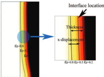
Fig.4. The β-phase volume fraction, εβ, is distributed continuously near the interface. We define the interface location at εβ= 0.5 and the interface thickness as the distance between εβ = 0.2and εβ = 0.8.

For comparison reasons, we also implemented an ALE simulation for this case. The ALE solution (ωAβ

and boundary location) is plotted in Fig.5. The solid– liquid boundary is represented explicitly, contrary to the diffuse interface under DIM. The computational domain expands to follow the moving of the interface. The ALE solution is used as a reference solution for DIM results. The detailed comparison of the interface locations between DIM and ALE will be presented in the section below. Before continuing the discussion, we must say a few words about the use of ALE simulation,

Fig. 4 εβdistribution under a DIM simulation: the location and

thickness of the diffuse interface

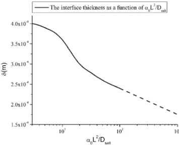
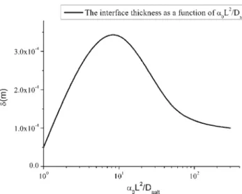
at least as it is implemented under COMSOL, i.e., without automatic remeshing. Surface imperfections are generated during the calculations due to severely deformed meshes. This may cause a non-convergence of the calculation. Therefore, one had to save data, remesh, and restart the computation after some small time. In short, the ALE simulation is very sensitive to the boundary geometry and the mesh shape. It works better for smooth interfaces and simple geometries, while the DIM is less sensitive to these aspects. The most important feature of DIM is the interface thick-ness, which mainly depends on the order of magnitude of the exchange coefficient. Figure6presents the inter-face thickness as a function of the non-dimensional ex-change coefficient number, α0L2/Dsaltat a same time, measured at the central cross section. L represents the domain width. For very small α0, the interface could not diffuse sufficiently as the solid–liquid mass exchange is very small. After a critical point, the increasing of α0 sharpens the interface thickness, with a limit ap-proaching to 0. In the limit α tends to infinity, when the solid phase is present, we obtain a so-called local equilibrium situation characterized by an infinitely thin interface and a concentration that reaches its equilib-rium concentration at the interface, i.e., the mathemat-ical solution of the original problems. Figure7, which presents the evolution of the interface displacement at the central cross section as a function of α0, shows that we need a limit value when increasing α0, e.g., around 50Dsalt/L2_{in this case. It is important to master these} aspects when using DIM results to avoid unphysical so-lutions. For details, an approximative convergence for the interface displacement is observed after a critical value of α0, where a plateau begins to rise with a very small slope. There seems to be a gap between the cur-rent DIM solution and the reference ALE result. While it is expected theoretically that the gap will decrease with very large α0, it must be emphasized that, depend-ing on the numerical algorithm, α0 cannot be taken as large as wanted since numerical difficulties may occur. For instance, if using operator splitting, the ODE sys-tem for the calculation of εβand ωAβbecomes very stiff

and may require very small time steps. In practice, the best choice would be to identify the plateau in Fig.7and takes a large enough α0, but not too large. Further, an optimization for the function shape for α could be made to improve the convergence and accuracy of DIM. This point will be discussed later in the paper. The time evolution of the interface thickness is also very impor-tant. Figure8 shows the interface evolution with time at the central cross section. We see that, after a short time evolution, the interface reaches a steady-state

Fig. 5 ωAβdistribution and

boundary location under the ALE (left) and DIM (right) simulations

value. This is an important feature of the DIM that the diffusion of the interface does not diverge. In practice, as shown in Fig.6, the interface thickness depends on α0. This is important also to quantify that since this will control mesh requirements (it is indeed necessary to have locally within the diffuse interface a small number of grid blocks, 3 seems to be an adequate minimum, numerically speaking). These simulations were carried out with a mesh size of 80 × 160. To study the mesh influence, Fig.9 compares the interface displacement for two mesh sizes 80 × 160 and 160 × 320. The results show a very good grid convergence.

Fig. 6 The interface thickness as a function of α0 at time t =

1,000 s

3.1.2 Interface displacement af fected by various exchange coef f icient functions

In the last section, the simulations were implemented using the exchange coefficient defined by Eq.28. This expression is obtained from the closure problem with a unit cell abstracted from a plane flow. However, this curve is not practical for numerical simulations, as it approaches infinity near 0 and has very steep derivative when εβ is small. Numerical divergence is easily aroused and a very small mesh size is required in such a case. Actually, since the choice for the effective

Fig. 7 The interface displacement as a function of α0at time t =

Fig. 8 The interface thickness as a function of time

coefficient is not highly constrained, without loss of significance, we tested new curves close to the recip-rocal shape. Among them, four simple and represen-tative curves will be used for comparison: (1) α = 4α0εβ ¡ 1− εβ¢, (2) α = α0 ³ 1− ε2 β ´ , (3) α = α0 ¡ 1− εβ¢, and (4) α = α0 ¡ 1− εβ ¢2

. Simulations are carried out using these curves, respectively. For all these four cases above, we find that the critical values of α0, which lead to an approximative convergence for the interface dis-placement, are on the order of 10Dsalt/L2. To guaran-tee the accuracy of the results, we use α0= 102Dsalt/L2 for all these cases. The comparison among different solutions is presented in Fig.10.

Fig. 9 Comparison of the interface location between the use of

80× 160and 160 × 320 mesh numbers

(a) Interface location at time t=1000s

(b) Interface displacement as a function of time

Fig. 10 Comparison of the interface displacement among

different exchange coefficients

The comparisons of the interface displacements show that the curve α = α0

¡ 1− εβ

¢2

provides the best solution compared to the reference (ALE solution). In fact, this curve has well inherited the features of the reciprocal curve, for instance, with large values at small εβ and small values at large εβ, with positive second-order gradients in the whole domain. There-fore, it is not surprising to obtain a good approximation using this curve. The curve α = α0ε−1β obtained from the analytical approach gives an error up to about 20 %. The reason is that the mass exchange coefficients are too small in most regions. For the other curves, there are about 5–10 % errors compared to the ref-erence solution. These errors are acceptable from a numerical point of view. Therefore, the curves such

as α = α0 ³ 1− εβ2 ´ and α = α0 ¡

1− εβ¢ are also good choices. We can also observe that the slope of the in-terface displacement with time in the reference solution is a little larger than that in the DIM simulations, with about 5 % difference between them. The reason is that in a practical DIM simulation, we could not use an infinite α0 to approach the ultimate convergence. However, this error is tolerable with engineering re-quirement, while one can also benefit from a much smaller numerical requirement. It must be emphasized here that we discuss this comparison at the beginning of the dissolution process. At this very beginning, we have for DIM a double process: the recession of the interface and the thickening of the interface. Because of the transient behavior for the interface thickness, the relative error interface thickness/interface displace-ment is relatively large at the beginning. However, since the interface thickness reaches a constant value, this relative error decreases with time (after t ≥ 1,000 s in the particular example).

In this paragraph, we discuss the definition of the in-terface location. The definition of the inin-terface location as εβ = 0.5 is somewhat instinctive. For a more strict identification, the interface location could be defined such that the integral of the solid volume fraction in the “liquid region” is equal to the integral of the liquid volume fraction in the “solid region”, e.g.,

Z Ä∈Ŵ− εσdV = Z Ä∈Ŵ+ εβdV (30)

where Ŵ represents the interface location, Ŵ− refers to the so called “liquid region”, and Ŵ+ refers to the so-called solid region. We plot the distributions of εβ and the mass exchange term Kβσ for different exchange coefficients in Fig.11.

For the case α = α0εβ−1, the interface is much more diffusive than for all the other cases. The reason is that dissolution is very slow in the region where εβ is large, resulting in a small amount of “solid mass fraction” lagging in the “liquid region.” The interface location can be roughly defined at εβ = 0.5. Concerning Kβσ, it is distributed irregularly, inclining toward the region where εβ is small and mass exchange is more active. In such a case, good numerical convergence may not be easily obtained. For the case α = α0

¡ 1− εβ

¢2 , the interface is also diffusive compared with the other three cases, with a long tail in the “liquid region.” The interface location defined by Eq.30is estimated to be at εβ = 0.6. On the contrary, it is interesting to see that the maximum of Kβσ is where εβ is nearly 0.4. This kind of asymmetry is also due to the small α in the region where

Fig. 11 Distributions of εβ and Kβσ under different exchange

coefficients at the central cross section at time t = 1,000 s

εβis large. Therefore, the interface location for this case should be dragged leftward in Fig. 10. That is to say, the interface location is not so close to the reference solution as that defined at εβ= 0.5. For the cases α = 4α0εβ ¡ 1− εβ¢, α = α0 ³ 1− ε2β ´ , and α = α0 ¡ 1− εβ¢, it is found that the distributions of εβand Kβσ are almost symmetric. Definitely, it is proper to define εβ = 0.5 as the interface location in these cases. In such cases, the numerical convergence will also be good due to the smooth and symmetric evolution of those diffuse quantities. Furthermore, by reviewing the comparison in Fig.10, we cannot distinguish a fundamental solution difference among these three cases. Anyhow, with the perspectives of inheriting the features from the func-tion α = α0εβ−1 obtained from the analytical approach, we recommend to adopt the function α = α0

³

1− εγ_β´, where γ is greater than 1.

The above simulations are under the condition Pe = 10, which could be regarded as advection-controlled flow. We would also like to study the effects of these

different curves under diffusion-controlled situations. Figure 12 plots the interface displacement with time in a pure diffusive case. It is shown that the displace-ment with the curve α = α0

¡ 1− εβ ¢2 , α = α0 ³ 1− ε2 β ´ , and α = α0 ¡

1− εβ¢ are all close to the ALE reference solution. One has to remember here that we look at the difference at the beginning of the dissolution process for which the interface thickening affects the interface location accuracy.

In summary, this section has intensively studied the influence of the exchange coefficients under several representative cases in both advection-controlled and diffusion-controlled situations. An optimum expres-sion, α = α0

³ 1− εβγ

´

, is proposed based on numeri-cal tests, considering both the accuracy and stability reasons. We remind the reader that, by construction, the DIM does not require a particular value for the transport parameters. There is a lot of flexibility and the above indications are given to illustrate the possible choices.

3.2 Simulation with gravity effects

Whenever density variation is present in the fluid phases, buoyancy forces can play an important role, arousing physical instabilities. In this section, we test the ability of DIM to reproduce these physical phenom-ena. Figure13presents the geometry used for the simu-lations with gravity. The length and width of the domain are 15 and 6 mm, respectively. Pure water is injected with a constant velocity (U0) into a channel whose walls are formed by two parallel salt blocks, resulting in the dissolution of the solid walls. Concerning the

Fig. 12 Comparison of the interface displacement for different

exchange coefficients in a pure diffusive case

Fig. 13 The geometry used for the simulation with gravity effects

velocity, with U0 = 1.0 × 10−6 m/s, the Péclet number calculated as Pe = U0L/Dsaltis close to unity, i.e., same importance of diffusion and advection mechanisms.

In this case, the dissolution of the salt walls results in higher concentrations around the interface than in other fluid regions. To characterize the gravity effects, we use the Rayleigh number, Ra, which is defined as the ratio of buoyancy forces to mass and momentum diffusivities

Ra = 1ρβmax|g|KmaxL µβDAβ

(31) Here, 1ρβmaxrepresents the difference of the maximum and minimum fluid densities, Kmaxrepresents the max-imum permeability, and L is the channel width.

Figure 14 plots the normalized mass fraction of species A, ÄAβ/ωeq. It shows that the symmetry of the flow and dissolution front is broken with impor-tant gravity effects. Gravity segregation appears at the cavity scale, and small-scale salt plumes are gener-ated within the upper mass transport boundary layer through a natural convection mechanism. It is remark-able that these salt plumes affect the interface dis-solution generating a rough interface. This kind of dissolution pattern was also observed experimentally [2,10,11].

Understanding the complex interaction of these roughnesses with the natural convection instabilities is beyond the scope of this paper, which is mainly on the model and its characteristics. In this section, we check that the convective structures do not suffer of numerical artifacts. In order to achieve this goal, we carried out several simulations with increasing α0. The simulation results for ÄAβ/ωeq are shown in Fig. 15. When α0 is large enough, e.g., larger than 50Dsalt/L2, the flow pattern does not change much with α0, i.e., we have similar wavelet and salt finger distributions. The interface displacement is also not affected. With the decrease of α0, e.g., when α0 = 10Dsalt/L2, the physical instabilities become smoothed, with fewer salt fingers and weaker tails. When α0 is very small, no

Fig. 14 Simulation results of

ÄAβ/ωeqwith time evolution

under Pe = 10 and Ra = 100

Fig. 15 Simulation results of

ÄAβ/ωeqwith different

magnitudes of α0at time t = 1,000 s

instability could be observed. The averaged thickness of the diffuse interface as a function α0 is plot in Fig.

16, showing that the averaged interface thickness is also reduced with the increase of α0. This explains the smoothing of the instabilities when the interface thickness becomes larger: The local Rayleigh number within the boundary layer becomes smaller. Therefore, the physical instabilities observed in the simulations can be regarded as physically sounded without numerical flaws provided a correct value is taken for α0.

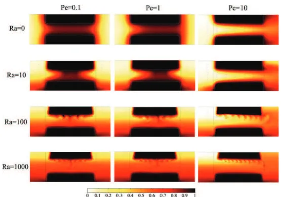
It is also interesting to see the influences of gravity for different Ra numbers and Pe numbers. Figure 17

plots a diagram of simulation results for various Ra and Pe. Figure17briefly exhibits the trends corresponding to Ra and Pe variations. When Ra is zero or small, the fluid flow is almost symmetric and stable. With the in-creasing of Ra, natural convection is gradually strength-ened and the physical instabilities become more and more strong and complex. In our examples, natural convection mostly happens around the upper interface rather than the bottom interface, as gravity and density gradients are in the same direction in the latter zone. Small-scale patterns, like wavelets around the inter-face, are observed. The number of wavelets increases when increasing the Ra number, greatly impacting the roughness of the interface during the dissolution. The

role of the Péclet number is complex. On one hand, disturbances may be advected outside the domain of interest, which would result in an apparent increase in stability. On the other hand, a larger Péclet number means a thinner boundary layer, with larger density gradients in favor of a strong salt fingering mechanisms. While we clearly see that, for low Ra number, the

Fig. 17 Diagram for Pe–Ra

tube-scale convective pattern is “washed” out of the do-main at large Péclet numbers, it does not mean that the occurrence of salt fingering is greatly affected at high Péclet numbers. Given the choice of a reference scale, i.e., the channel diameter, the geometry depends on a dimensionless ratio A. We did not explore different values of this ratio. Our particular choice A = 5 cor-responds to a channel of relatively large extension, in order to be able to obtain several natural convection patterns at large Raleigh numbers. A thorough study of the impact of this parameter has to be undertaken but is beyond the scope of this paper. While the study of hydrodynamic instabilities has been very popular in many different domains, the coupling of natural convection and dissolution has received less attention and will remain our objective in future studies. We did not explore here very large Peclet numbers. In terms of the characteristics of the Pe–Ra diagram, we think that the various pattern limits have been explored. Higher Pe values would increase the “instability washing out” mechanism. However, very large Pe numbers will pro-duce very thin boundary layers, and it will be necessary to verify that the interface thickness does not affect the accuracy of the dissolution modeling.

4 Conclusion

For simulations of the solid–liquid dissolution process, one can use either explicit treatment methods

(rep-resented by ALE in this paper) or diffuse interface methods (a local non-equilibrium DIM in this paper). ALE methods face difficulties when solving problems with complex interfaces, e.g., sharp angles, complex pore structures, as it relies strongly on the mesh shape. On the contrary, the DIM methods are easier to imple-ment for simulating dissolution problems, as the whole domain is described through a phase field (volume fraction of liquid phase in this paper). In this paper, adopting the idea from [15], a local non-equilibrium diffuse interface model based on a porous medium theory is extended to study dissolution problems with density variations taken into account. A closure prob-lem is solved with a unit cell abstracted from a plane flow to obtain the effective coefficients for the aver-aged equations, e.g., effective diffusion coefficient D∗

Aβ,

exchange coefficient α. Several numerical tests with a plane-flow geometry were carried out to study the features of DIM simulations, for instance, the influence of the exchange coefficient magnitude and shape on the diffuse interface thickness and displacement. An “optimum” expression for the exchange coefficient was obtained by looking at the agreement between the DIM solutions and the reference ALE solutions.

Numerical tests showed the ability of DIM computa-tions to reproduce conveniently flows with strong den-sity variations, i.e., large Rayleigh numbers. Unstable flows producing salt fingers and interface wavelets were observed as a function of the Rayleigh number, Ra. Computations showed also the impact of the Péclet

number on the instabilities dynamic. A diagram illus-trating the Ra–Pe interactions was proposed for flow in a tube-like domain.

It must be mentioned here that non-traditional terms in the macro-scale transport equations have been ne-glected in this study. Some non-linearities and depen-dences have also been discarded, like for instance dis-persion mechanisms (Taylor disdis-persion for the plane unit cell). Would they improve the simulations, for instance by leading to a better convergence? We have not found evidence in preliminary tests. Of course, this is a different matter when the local non-equilibrium model is used for a true porous medium application, as illustrated in [14], for which the effective properties must be estimated accurately.

A further advantage of using a diffuse interface model is that it allows us to introduce easily auto-matic remeshing algorithms, such as adaptive mesh refinement (AMR) algorithms, which can greatly im-prove the calculation speed, since very fine meshes are required near the interface. The AMR algorithm for 2D and 3D simulations using the local non-equilibrium DIM will be presented in a subsequent paper.

Acknowledgment The authors would like to thank INERIS for the financial support.

Appendix A: Upscaling of the balance equations

Substituting Eqs.13and14into Eq.18, we have ∂­ρβωAβ ® ∂t | {z } [a]accumulation + ∇ ·­ρβωAβvβ ® | {z } [b]advection = ∇ ·­ρβDAβ∇ωAβ ® | {z } [c]diffusion −1 V Z Aβσ nβσ · ρβ ¡ vβ− w¢ dA | {z } [d]phase exchange (32) We introduce the deviations of the mass fraction and velocity, respectively, by

˜

ωAβ = ωAβ− ÄAβ (33)

˜vβ = vβ− εβ−1Vβ (34)

Using a Taylor’s series expansion, terms involving the density may be written

­ ρβωAβ ® =Dρβ ³­ ωAβ ®β + ˜ωAβ ´ ωAβ E = ¿µ ρβ ³­ ωAβ ®β´ + ∂ρβ ∂ωAβ ˜ ωAβ+ · · · ¶ ωAβ À (35) In Eq. 35, it can be demonstrated using the clas-sical theory of dispersion that ∂ρβ

∂ωAβω˜Aβ has the order

of O¡l

LÄAβ¢, so that when satisfying the constraint

O¡_LlÄAβ

¢ ≪ ρβ

¡

ÄAβ¢, Eq.35can be simplified to

¿µ ρβ ¡ ÄAβ ¢ + ∂ρβ ∂ωAβ ˜ ωAβ+ · · · ¶ ωAβ À =­ρβ ¡ ÄAβ ¢ ωAβ ® (36) Implementing a Taylor’s expansion again for the spatial variations of the averaged quantities, we have ­ ρβ ¡ ÄAβ ¢ ωAβ ® = ¿ ρβ µ ÄAβ|x+y · ∇ÄAβ+ 1 2y y : ∇∇ÄAβ+ · · · ¶ ωAβ À (37) Following the analysis of [28], Eq.37can be simplified to ¿ ρβ µ ÄAβ|x+y · ∇ÄAβ+ 1 2y y : ∇∇ÄAβ+ · · · ¶ ωAβ À =­ρβ ¡ ÄAβ|x ¢ ωAβ ® = ρβ ¡ ÄAβ ¢ ­ ωAβ ® = εβρβ ¡ ÄAβ ¢ ÄAβ (38)

thus we can make the following simplification ­ ρβωAβ ® = εβρβ∗ÄAβ (39) where ρ∗ βrepresents ρβ ¡ ÄAβ¢.

Similarly, we can also obtain the simplifications: ­ ρβωAβvβ ® = ρ_β∗­ωAβvβ ® (40) ­ ρβDAβ∇ωAβ ® = ρβ∗ ­ DAβ∇ωAβ ® (41) This enables us to extend the term [a] in Eq.32as [a] = µ εβρβ∗ ∂ÄAβ ∂t + ÄAβ ∂εβρ∗β ∂t ¶ (42)

Term [b] can be extended as [b ] = ∇ ·­ρβωAβvβ ® = ∇ ·¡ρ_β∗­ωAβvβ ®¢ = ∇ ·¡ρ_β∗¡ÄAβVβ+ ­ ˜ ωAβvβ ®¢¢ = ÄAβ∇ · ¡ ρ_β∗Vβ ¢ +¡ρ_β∗Vβ ¢ · ∇ÄAβ + ρ∗β∇ · ­ ˜ ωAβ˜vβ ® +­ω˜Aβ˜vβ ® · ∇ρβ∗ (43) Term [c] can be extended as

[c] = ∇ ·­ρβDAβ∇ωAβ ® = ∇ ·¡ρ_β∗­DAβ∇ωAβ ®¢ = ∇ ·   ρ ∗ βDAβ   ∇ ¡ εβÄAβ ¢ + 1 V Z Aβσ nβσωAβd A       (44) = ∇ ·   ρ ∗ βDAβ   εβ∇ÄAβ+ 1 V Z Aβσ nβσω˜Aβd A       (45) According to Eqs.16–17, term [d] can be extended as [d] = Kβσ = −1 V Z Aβσ nβσ · ρβ ¡ vβ− w¢ dA = 1 V Z Aβσ nβσ · ρβDAβ ¡ 1− ωAβ ¢ ∇ ωAβd A (46)

where Kβσ represents the exchange term between the σ-phase and the β-phase.

In a whole, Eq.32can be written as,

εβρβ∗ ∂ÄAβ ∂t + ÄAβ ∂εβρβ∗ ∂t + ÄAβ∇ · ¡ ρ_β∗Vβ ¢ +¡ρ_β∗Vβ ¢ · ∇ÄAβ + ρβ∗∇ · ­ ˜ ωAβ˜vβ ® +­ω˜Aβ˜vβ ® · ∇ρβ∗ = ∇ · ρ∗βDAβ   εβ∇ÄAβ+ 1 V Z Aβσ nβσω˜Aβd A    +Kβσ (47)

Similarly, we can also write the averaged form of the total mass continuity equation (Eq.1) as,

∂εβρβ∗ ∂t + ∇ · ¡ ρ_β∗Vβ ¢ =Kβσ (48)

Subtract ÄAβ×Eq.48to Eq.47, we obtain the

aver-aged form of the balance equation as follows: εβρβ∗ ∂ÄAβ ∂t + ¡ ρ_β∗Vβ ¢ · ∇ÄAβρβ∗∇ · ­ ˜ ωAβ˜vβ ® +­ω˜Aβ˜vβ ® · ∇ρβ∗ = ∇ ·   ρ ∗ βDAβ   εβ∇ÄAβ+ 1 V Z Aβσ nβσω˜Aβd A       +¡1− ÄAβ ¢ Kβσ (49) where Kβσ = 1 V Z Aβσ nβσ· ρβDAβ ¡ 1− ωAβ ¢ ∇ ÄAβd A +1 V Z Aβσ nβσ · ρβDAβ ¡ 1− ωAβ ¢ ∇ ˜ωAβd A (50)

In order to develop an equation for the deviation of the mass fraction, we firstly subtract ωAβ×Eq.1from

Eq.2and obtain ∂ωAβ ∂t + vβ· ∇ωAβ= ∇ · ¡ ρβDAβ∇ωAβ ¢ (51) Subtracting Eq.49׳εβρβ∗ ´−1 to Eq.51, we have ∂ ˜ωAβ ∂t +˜vβ· ∇ÄAβ+ vβ· ∇ ˜ωAβ = ε−1β ∇ · ­ ˜ ωAβ˜vβ ® +¡εβρβ∗ ¢−1­ ˜ ωAβ˜vβ ® · ∇ρ∗β + 1 ρ_β∗∇ · ¡ ρ_β∗DAβ∇ ˜ωAβ ¢ + 1 ρ_β∗∇ · £¡ ρ_β∗− ρβ ¢ DAβ∇ωAβ ¤ +¡εβρ∗β ¢−1 ∇ · ρβ∗DAβ    1 V Z Aβσ nβσω˜Aβd A    −¡εβρβ∗ ¢−1¡ 1− ÄAβ ¢ Kβσ (52)

For l ≪ L, it can be assumed that ε_β−1∇ ·­ω˜Aβ˜vβ ® ≪ vβ· ∇ ˜ωAβ (53) ε_β−1∇ ·   ρ ∗ βDAβ 1 V Z Aβσ nβσω˜Aβd A    ≪ ∇ ·¡ρ_β∗DAβ∇ ˜ωAβ ¢ (54) It is also assumed that

¡ εβρβ∗ ¢−1­ ˜ ωAβ˜vβ ® · ∇ρβ∗≪ ε −1 β ∇ · ­ ˜ ωAβ˜vβ ® (55) 1 ρ∗ β ∇ ·£¡ρ_β∗− ρβ ¢ DAβ∇ωAβ ¤ ≪ 1 ρ∗ β ∇ ·¡ρ_β∗DAβ∇ ˜ωAβ ¢ (56) Then we can simplify Eq.52to

∂ ˜ωAβ ∂t + ˜vβ· ∇ÄAβ+ vβ· ∇ ˜ωAβ = 1 ρ_β∗∇ · ¡ ρ_β∗DAβ∇ ˜ωAβ ¢ −¡εβρβ∗ ¢−1 1 V Z Aβσ nβσ · ρβDAβ∇ ˜ωAβ 1− ωeq d A (57)

We suppose that, in a unit cell, ρβ≃ ρβ∗, so that the last term of the above equation can be replaced by

¡ εβρβ∗ ¢−1 1 V Z Aβσ nβσ· ρβDAβ∇ ˜ωAβ 1− ωeq d A =¡εβ ¢−1 1 V Z Aβσ nβσ · DAβ∇ ˜ωAβ 1− ωeq d A (58)

In Eqs.49 and57, non-homogeneous terms can be viewed as source terms for ˜ωAβ, so that ˜ωAβ can be

represented by the following expression according to [27] analysis:

˜

ωAβ =bβ· ∇ÄAβ+sβ(ωeq− ÄAβ) (59)

where bβ and sβ are the mapping variables of the closure problem of the mass fraction deviation. They obey two different closure problems (problem Ia and problem Ib) approximating Eq. 57 as presented be-low. In practice, starting with the work [15], we need to couple problems Ia and Ib, i.e., sβ appears in problem Ia. Problem Ia ˜vβ+ vβ· ∇bβ = ∇ · ¡ DAβ∇bβ ¢ − ε−1_β 1 V Z Aβσ nβσ ·DAβ∇bβd A (60) BC1 bβ = 0at Aβσ (61) bβ ¡ r + li ¢ =bβ(r) , i = 1, 2, 3 (62) ­ bβ ®β = 0 (63) Problem Ib vβ· ∇sβ= ∇ · ¡ DAβ∇sβ ¢ − 1 V Z Aβσ nβσ ·DAβ∇sβd A (64) BC2 sβ= 1at Aβσ (65) sβ¡r + li ¢ =sβ(r) , i = 1, 2, 3 (66) ­ sβ®β = 0 (67)

Using these above forms in Eq. 49 leads to the following averaged equation form for the dissolution problem: εβρβ∗ ∂ÄAβ ∂t + ρ ∗ β(Vβ− (1 − ÄAβ)u1β+DAβ∇εβ) · ∇ÄAβ− ρβ∗∇ · ¡ dβÄAβ ¢ = ∇ ·³εβρβ∗D∗Aβ· ∇ÄAβ ´ + (1 − ÄAβ)Kβσ (68) with u1β = 1 ρ_β∗ 1 V Z Aβσ ρβ ¡ 1− ωeq¢ D Aβnβσ ·£∇bβ+ ¡ 1−sβ¢I¤ dA (69) dβ= − 1 V Z Aβσ DAβ ¡ nβσsβ¢ dA + ­sβ˜vβ ® (70)

D∗_Aβ = εβDAβ    I + ε −1 β 1 V Z Aβσ ¡ nβσbβ¢ dA    − ε−1_β ­bβ˜vβ ® (71) Kβσ =£α1+ (1 − ÄAβ)−1α2 ¤ (ωeq− ÄAβ) (72) α1= 1 V Z Aβσ ρβ ¡ 1− ωeq ¢ DAβ ¡ nβσ· ∇sβ¢ dA (73) α2= ∇ρβ∗· ­ sβ˜vβ ® (74) Since our only goal is to obtain a diffuse interface model, it is not necessary to keep all the features of the Darcy-scale non-equilibrium model. Therefore, in order to simplify the diffuse interface model, we neglect the terms u1β, dβ, α2 and DAβ∇εβ. Consequently, Eq.

75can be simplified as εβρβ∗ ∂ÄAβ ∂t + ρ ∗ βVβ· ∇ÄAβ = ∇ ·³ρ_β∗D∗_Aβ· ∇ÄAβ ´ + (1 − ÄAβ)Kβσ (75) where Kβσ =    1 V Z Aβσ ρβ ¡ 1− ωeq ¢ DAβ ¡ nβσ · ∇sβ¢ dA    סωeq− ÄAβ ¢ = α(ωeq− ÄAβ) (76)

Concerning the σ -phase, the upscaling method ap-plied to Eq.4leads to

∂εσhρσiσ ∂t = 1 V Z Aβσ ρσnσβ· wd A (77)

Since ρσ is a constant and εβ+ εσ = 1, according to Eq.9, we rewrite the last equation as

ρσ ∂εβ ∂t = 1 V Z Aβσ nβσ · wd A = Kβσ. (78)

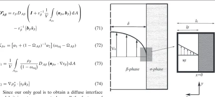
Appendix B: Analysis for the effective coefficients

To obtain the estimates of the effective coefficients for solid–liquid dissolution problems, we consider a simple unit cell as represented in Fig18. εβcould be computed as lβ/lc, where lcis regarded as the characteristic length of the unit cell.

Fig. 18 A unit cell used for solid–liquid interface dissolution

In a domain including the interface, we have mass and momentum boundary layers that develop (Fig.18), and we will make the simplification in the unit cell that the velocity vβ has a linear distribution against x in the unit cell. Therefore, we have the following expressions for vβ:

vβ =V0x/δ =PeDAβx/δ2 (79)

Replacing this equation into the closure problems Eqs.60–67, we are able to obtain the solutions for the closure variables, bβand sβ, expressed as,

bβx= 0 (80) bβy= Pe³16X3_{− 21ε} βX2+ 6ε2βX ´ 96η (81) sβ= ³ 3X2 − 6εβX + 2εβ2 ´ 2ε2 β (82) where X = x/lcand η = δ/lc.

Substituting the last three equations into Eq. 71

and Eq.73, we have the following expressions for the effective diffusion coefficient and the exchange term,

D∗ Aβ=   εβDAβ 0 0 εβDAβ µ 1+ Pe 2_ε4 β 1920η2 ¶   (83) α = 3 l2 cεβ DAβ (84)

The effective permeability can also be obtained by the traditional upscaling,

K = ε 2 β 3l2 c I. (85)

Appendix C: 1D analytical solution of DIM equations

We define a diffuse interface zone ZDI with thickness

δ, where the left boundary approximates εβ = 0and the right boundary approximates εβ = 1. When the mass exchange coefficient α is infinite, δ approaches to 0 and ÄAβ approaches to ωeq in ZDI. Consequently, an integration of Eq.22over ZDIleads to,

ρσδ dεβ dt =Kβσ (86) where Kβσ = R ZDIρβα ¡

ωeq− ÄAβ¢ dZ is the

integra-tion of the mass exchange in ZDI. According to the mass balance, the speed of moving boundary w can be expressed as,

w= −δdεβ

dt (87)

Equations86and87lead to the following relation, w= − 1

ρσ

Kβσ (88)

Integrating of Eq.21over ZDI, we have − ρβw+ ¡ ρβVβ ¢ |Z+ Z− = −ρβw+ ¡ ρβVβ ¢ Z+− ¡ ρβVβ ¢ Z−=Kβσ (89)

Since Vβ equals zero in the solid domain and equals

V (velocity going out of the interface) in the liquid domain, Eq.89can be rewritten as,

−ρβw+ ρβV = Kβσ (90)

Multiply Eq. 21 with ÄAβ and add to Eq. 23, then

integrating over ZDI, we have ∂εβρβÄAβ ∂t δ + ¡ ρβVβÄAβ ¢¯ ¯Z+ Z− =¡εβρβDAβ∇ÄAβ ¢¯ ¯Z+ Z−+Kβσ (91) or

−ÄAβρβw+ ÄAβρβV = ρβDAβ∇ÄAβ+Kβσ (92)

Arranging Eqs.88,90, and92, we have w= ρβ

ρσ(1 − ωeq)

DAβ∇ÄAβ (93)

which has the same form as Eq.16.

References

1. Anderson, D.M., McFadden, G.B.: Diffuse-interface meth-ods in fluid mechanics. Annu. Rev. Fluid Mech. 30, 139–165 (1998)

2. Anderson, R.Y., Kirkland, D.W.: Dissolution of salt deposits by brine density flow. Geology 8, 66–69 (1980)

3. Beckermann, C., Diepers, H.-J., Steinbach, I., Karma, A., Tong, X.: Modeling melt convection in phase-field simula-tions of solidification. J. Comput. Phys. 154, 468–496 (1999) 4. Bekri, S., Thovert, J.F., Adler, P.M.: Dissolution of porous

media. Chem. Eng. Sci. 50, 2765–2791 (1995)

5. Boettinger, W.J., Warren, J.A., Beckermann, C., Karma, A.: Phase-field simulation of solidification. Annu. Rev. Mater. Res. 32, 163–194 (2002)

6. Bousquet-Melou, P., Neculae, N., Goyeau, B., Quintard, M.: Averaged solute transport during solidification of a binary mixture: active dispersion in dendritic structures. Metall. Mater. Trans. B 33, 365–376 (2002)

7. Cahn, J.W., Hilliard, J.: Free energy of a nonuniform sys-tem. I. Interfacial free energy. J. Chem. Phys. 28, 258–267 (1958)

8. Collins, J.B., Levine, H.: Diffuse interface model of diffusion-limited crystal growth. Phys. Rev. B 31, 6119–6122 (1985)

9. Dell’Isola, F., Gouin, H., Rotoli, G.: Nucleation of spheri-cal shell-like interfaces by second gradient theory: numerispheri-cal simulations. Eur. J. Mech. B Fluid 15, 545–568 (1996) 10. Dijk, P.E., Berkowitz, B.: Buoyancy-driven dissolution

enhancement in rock fractures. Geology 28, 1051–1054 (2000)

11. Dijk, P.E., Berkowitz, B., Yechieli, Y.: Measurement and analysis of dissolution patterns in rock fractures. Water Re-sour. Res. 38 (2002). doi:10.1029/2001WR000246

12. Donea, J., Giuliani, S., Halleux J.P.: An arbitrary Lagrangian–Eulerian finite element method for transient dynamic fluid–structure interactions. Comput. Methods Appl. Mech. Eng. 33, 689–723 (1982)

13. Glimm, J., Grove, J.W., Li, X.L., Shyue, K.M., Zeng, Y., Zhang, Q.: Three-dimensional front tracking. SIAM J. Sci. Comput. 3, 703–727 (1998)

14. Golfier, F., Quintard, M., Whitaker, S.: Heat and mass trans-fer in tubes: an analysis using the method of volume averag-ing. J. Porous Media 5(3), 169–185 (2002)

15. Golfier, F., Zarcone, C., Bazin, B., Lenormand, R., Lasseux, D., Quintard, M.: On the ability of a Darcy-scale model to capture wormhole formation during the dissolution of a porous medium. J. Fluid Mech. 457, 213–254 (2002)

16. Hirt, C.W., Nicolas, B.D.: Volume of fluid (VOF) method for the dynamics of free boundaries. J. Comput. Phys. 39, 201– 225 (1981)

17. Kang, Q., Zhang, D., Chen, S.: Simulation of dissolution and precipitation in porous media. J. Geophys. Res. 108, 2505 (2003). doi:10.1029/2003JB002504

18. Kovacevic, I., Sarlera, B.: Solution of a phase-field model for dissolution of primary particles in binary aluminum alloys by an r-adaptive mesh-free method. Mater. Sci. Eng. A 413, 423– 428 (2005)

19. Leo, P.H., Lowengrub, J.S., Jou, H.J.: A diffuse interface model for microstructural evolution in elastically stressed solids. Acta Mater. 46, 2113–2130 (1998)

20. Lopez, J., Hernandez, J., Gomez, P., Faura, F.: An improved PLIC-VOF method for tracking thin fluid structures in in-compressible two-phase flows. J. Comput. Phys. 208(1), 51–74 (2005)