Comparative study of infrared thermography, ultrasonic
C-scan, X-ray computed tomography and terahertz
imaging on composite materials
Thèse
Hai Zhang
Doctorat en génie électrique
Philosophiæ doctor (Ph. D.)
Comparative study of infrared thermography,
ultrasonic C-scan, X-ray computed tomography and
terahertz imaging on composite materials
Thèse
Hai Zhang
Sous la direction de:
Résumé
L’évaluation non destructive (NDT) des matériaux composites est compliquée en raison de la vaste gamme de défauts rencontrés (y compris délaminage, microfissuration, fracture de la fibre, retrait des fibres, fissuration matricielle, inclusions, vides et dommages aux chocs). La capacité de caractériser quantitativement le type, la géométrie et l’orientation des défauts est essentielle. La thermographie infrarouge (IRT), en tant que technique de diagnostic d’image, peut satisfaire le besoin industriel croissant de NDT&E.
Dans la thèse, la thermographie par excitation optique et mécanique a été utilisée pour étu-dier différents matériaux composites, dont 1) des préformes sèches en fibres de carbone, 2) des composites de fibres naturelles, 3) des composites hybrides de basalte-fibres de carbone soumis à une charge d’impact (séquence de type sandwich et séquence d’empilement intercalé), 4) des défauts micro-dimensionnés dans un composite polymère renforcé de fibre de carbone (CFRP) en 3D avec une couture de type « joint en T », et 5) des peintures sur toile qui peuvent être considérées comme des matériaux composites. Une nouvelle technique IRT de thermo-graphie de ligne par micro-laser (micro-LLT) a été proposée pour l’évaluation des porosités submillimétriques dans le CFRP. La microscopie de points par micro-laser (micro-LST) et la micro-vibrothermographie (micro-VT) ont également été présentées avec l’utilisation de mi-crolentilles. La thermographie pulsée (PT) et la thermographie modulée « à verrouillage » (LT) ont été comparées à la tomographie par rayons X (TC) pour validation. Le C-scan ultrasonore (UT) et l’imagerie par ondes tera-hertziennes en onde continue (CW THz) ont également été réalisés à des fins comparatives. L’inspection par techniques thermographiques est une question ouverte à discuter pour le public scientifique. En fait, la thermographie par impulsions (PPT) basée sur la transformation de phase a été utilisée pour estimer la profondeur des dommages. Pour traiter les données thermographiques, on a également utilisé la reconstruction de signal thermographique de base (B-TSR), la thermographie des composants principaux (PCT) et la thermographie des moindres carrés partiels (PLST). Enfin, une analyse complète et compa-rative basée sur le diagnostic d’images thermographiques a été menée en vue d’applications industrielles potentielles.
Abstract
Non-destructive testing (NDT) of composite materials is complicated due to the wide range of flaws encountered (including delamination, micro-cracking, fiber fracture, fiber pullout, matrix cracking, inclusions, voids, and impact damage). The ability to quantitatively characterize the type, geometry, and orientation of flaws is essential. Infrared thermography (IRT), as an image diagnostic technique, can satisfy the increasing industrial need for NDT&E.
In the thesis, optical and mechanical excitation thermography were used to investigate differ-ent composite materials, including 1) carbon fiber dry preforms, 2) natural fiber composites, 3) basalt-carbon fiber hybrid composites subjected to impact loading (sandwich-like and interca-lated stacking sequence), 4) micro-sized flaws in a stitched T-joint 3D carbon fiber reinforced polymer composite (CFRP), and 5) paintings on canvas which can be considered as com-posite materials. Of particular interest, a new IRT technique micro-laser line thermography (micro-LLT) was proposed for the evaluation of submillimeter porosities in CFRP. Micro-laser spot thermography (micro-LST) and micro-vibrothermography (micro-VT) were also presented with the usage of a micro-lens. Pulsed thermography (PT) and lock-in thermogra-phy (LT) were compared with x-ray computed tomograthermogra-phy (CT) for validation. Ultrasonic C-scan (UT) and continuous wave terahertz imaging (CW THz) were also conducted for the comparative purpose. The inspection by thermographic techniques is an open matter to be discussed for the scientific audience. In fact, pulse phase thermography (PPT) based on phase transform was used to estimate the damage depth. Basic thermographic signal reconstruction (B-TSR), principal component thermography (PCT) and partial least squares thermography (PLST) (another more recent advanced image processing technique) were also used to pro-cess the thermographic data. Finally, a comprehensive and comparative analysis based on thermographic image diagnostics was conducted in view of potential industrial applications.
Contents
Résumé iii
Abstract iv
Contents v
List of Tables vii
List of Figures viii
Acknowledgements xvii
Introduction 1
1 A Review of NDT&E techniques 4
1.1 Optical Excitation Thermography in this research . . . 4
1.2 Mechanical Excitation Thermography . . . 5
1.3 Ultrasonic C-scan (UT) . . . 6
1.4 X-ray Computed Tomography (CT) . . . 6
1.5 Continuous Wave Terahertz Imaging (CW THz). . . 7
2 Infrared Image Processing 9 2.1 Pulsed Phase Thermography (PPT) . . . 9
2.2 Partial Least Square Thermography (PLST) . . . 10
2.3 Principal Component Thermography (PCT) . . . 12
2.4 Basic Thermographic Signal Reconstruction (B-TSR) . . . 14
2.5 Cold Image Subtraction (CIS) . . . 15
3 Image Diagnosis for Industrial Carbon Fiber Dry Preform 16 3.1 Introduction. . . 16
3.2 Carbon Fiber Dry Preforms . . . 17
3.3 Experimental Configurations . . . 19
3.4 Experimental Measurement for Thermal Diffusivity . . . 20
3.5 Experimental Results and Analysis . . . 22
3.6 Summary . . . 26
4 Image Diagnosis and Characterization for Natural Fiber Composites 30 4.1 Introduction. . . 30
4.3 Experimental Configurations . . . 33
4.4 Experimental Results and Analysis . . . 36
4.5 Summary . . . 42
5 Image Diagnostics of Impact Damage in Basalt and Carbon Fiber Com-posites 45 5.1 Introduction. . . 45
5.2 Basalt-Carbon Hybrid Composites . . . 46
5.3 Experimental Configurations . . . 47
5.4 Experimental Results and Analysis . . . 48
5.5 Summary . . . 55
6 Image Diagnosis for Micro-sized Flaws in CFRP 57 6.1 Introduction. . . 57
6.2 T-joint CFRP . . . 59
6.3 Inspection Results Using the Established Techniques . . . 61
6.4 Micro Laser Line Thermography (Micro-LLT) . . . 67
6.5 Lock-in Micro-LLT and Micro-LST . . . 76
6.6 Micro-vibrothermoraphy (Micro-VT) . . . 79
6.7 Summary . . . 82
7 Non-destructive Investigation of Paintings on Canvas 84 7.1 Introduction. . . 84
7.2 Description of The Samples . . . 87
7.3 Experimental Configurations . . . 88 7.4 Result Analysis . . . 91 7.5 Summary . . . 94 Conclusion 96 A List of contributions 98 Bibliography 101
List of Tables
3.1 Orientation/width of layers and defects. . . 18
3.2 Thermal diffusivity by theoretical calculation and experimental measurement. . 21
3.3 Relationship between modulated frequency fb and detection depth z. . . 22
3.4 Performance of thermographic methods. . . 28
4.1 Dent depth as a function of impact energy. . . 33
4.2 Flir Phoenix (MWIR) technical specifications [1]. . . 34
4.3 Physical properties of materials. . . 36
4.4 Relationship between modulated frequency fb and depth z. . . 42
4.5 Capabilities of different techniques. . . 44
5.1 Thickness and fiber volume fraction of specimens. . . 46
5.2 Damaged areas obtained from PCT in PT and VT. . . 49
5.3 Damaged areas obtained from PLST. . . 50
5.4 Calculated thermal diffusivity α. . . 51
5.5 Relationship between modulated frequency fb and depth z. . . 52
5.6 Damaged areas obtained from PPT and LT. . . 53
6.1 The model geometrical parameters . . . 61
6.2 The material properties . . . 70
6.3 Detection capacity of pulsed micro-LLT. . . 76
6.4 Micro-VT generator technical specifications. . . 79
List of Figures
2.1 Schematic representation of the transformation of the 3D thermal data into a
2D raster-like matrix. . . 12
2.2 (a) Thermographic data rearrangement from a 3D sequence to a 2D A matrix in order to apply SVD, (b) rearrangement of 2D U matrix into a 3D matrix
containing the EOFs [2]. . . 13
2.3 Typical use of TSR (model: 8 plies CFRP (0.0125” / ply)) [3] . . . 14
2.4 An example with an academic aluminum plate to explain cold image subtraction. 15
3.1 Photographs of TW and PW specimens: (a) TW-01: front side, (b) TW-02: front side, (c) PW-01: front side, (d) TW-01: rear side, (e) TW-02: rear side,
(f) PW-01: rear side. . . 17
3.2 Photographs of US specimens: (a) US-01: front side, (b) US-02: front side, (c)
US-03: front side, (d) US-01: rear side, (e) US-02: rear side, (f) US-03: rear side. 18
3.3 Optical excitation thermography set-ups: (a) schematic set-up for PT using flashes, (b) schematic up for PT and LT using lamps, (c) experimental
set-up for PT using flashes, (d) experimental set-set-up for PT and LT using lamps. . 19
3.4 (a) Experimental measurement set-up, (b) an example for the α calculation. . . 21
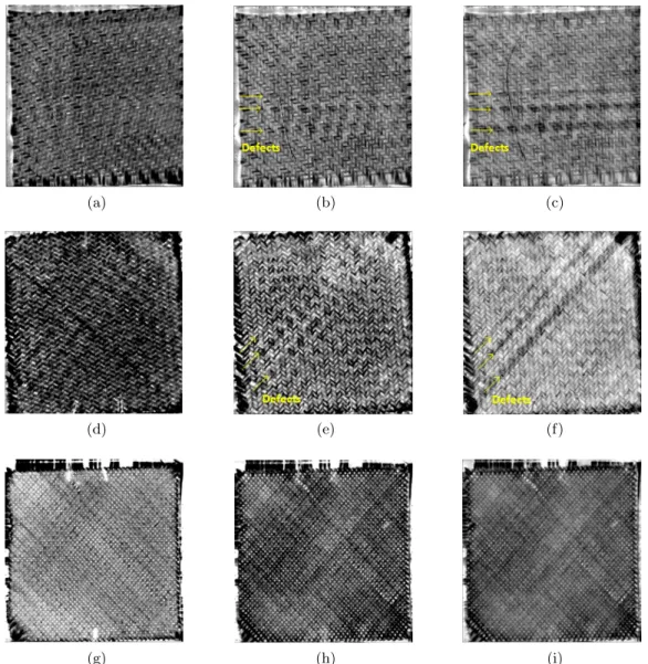
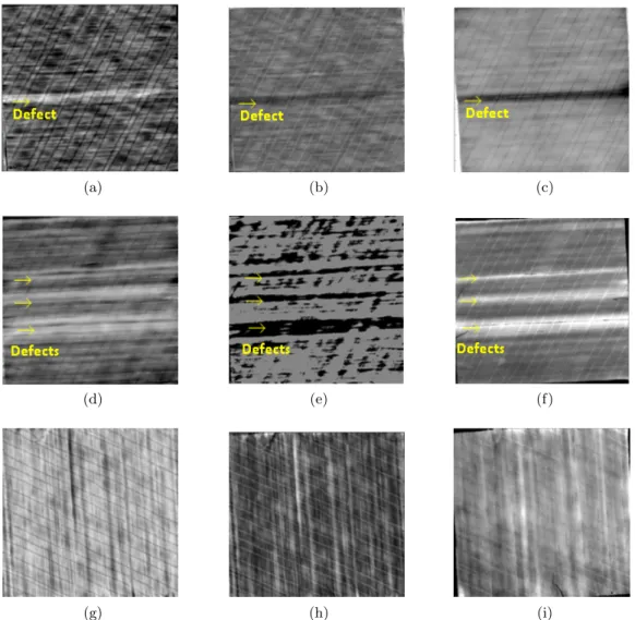
3.5 Phase transform results of TW/PW specimens using the flashes set-up and 88 fps: (a) 01: 0.25 mm, (b) 01: 0.4 mm, (c) 01: 0.5 mm, (d) TW-02: 0.25 mm, (e) TW-TW-02: 0.4 mm, (f) TW-TW-02: 0.5 mm, (g) PW-01: 0.25 mm,
(h) PW-01: 0.4 mm, (i) PW-01: 0.5 mm. . . 23
3.6 B-TSR and PCT results of TW/PW specimens using the flashes set-up and 88 fps: (a) TW-01: B-TSR (1st), (b) TW-01: B-TSR (2nd), (c) TW-01: PCT (EOF03), (d) TW-02: B-TSR (1st), (e) TW-02: B-TSR (2nd), (f) TW-02: PCT (EOF03), (g) PW-01: B-TSR (1st), (h) PW-01: B-TSR (2nd), (i) PW-01: PCT
(EOF01). . . 24
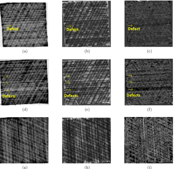
3.7 PLST results of TW/PW specimens using the flashes set-up and 88 fps: (a) TW-01: 1st loading, (b) TW-01: 2nd loading, (c) TW-01: 3rd loading, (d) TW-02: 1st loading, (e) TW-02: 2nd loading, (f) TW-02: 3rd loading, (g)
PW-01: 1st loading, (h) PW-01: 2nd loading, (i) PW-01: 3rd loading. . . 25
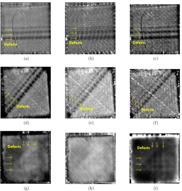
3.8 Phase transform results of US specimens using the flashes set-up and 88 fps: (a) US-01: 0.15 mm, (b) US-01: 0.3 mm, (c) US-01: 0.4 mm, (d) US-02: 0.15 mm, (e) US-02: 0.3 mm, (f) US-02: 0.4 mm, (g) US-03: 0.15 mm, (h) US-03:
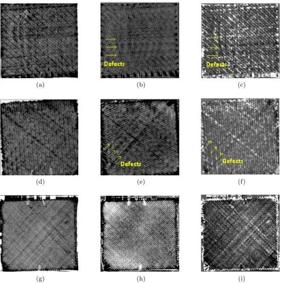
3.9 B-TSR and PCT results of US specimens using the flashes set-up and 88 fps: (a) US-01: B-TSR (1st), (b) US-01: B-TSR (2nd), (c) US-01: PCT (EOF01), (d) US-02: B-TSR (1st), (e) US-02: B-TSR (2nd), (f) US-02: PCT (EOF01),
(g) US-03: B-TSR (1st), (h) US-03: B-TSR (2nd), (i) US-03: PCT (EOF01). . 27
3.10 PLST results of US specimens using the flashes set-up and 88 fps: (a) US-01: 1st loading, (b) US-01: 3rd loading, (c) US-01: 5th loading, (d) US-02: 1st loading, (e) US-02: 3rd loading, (f) US-02: 5th loading, (g) US-03: 1st loading,
(h) US-03: 3rd loading, (i) US-03: 5thUS loading.. . . 28
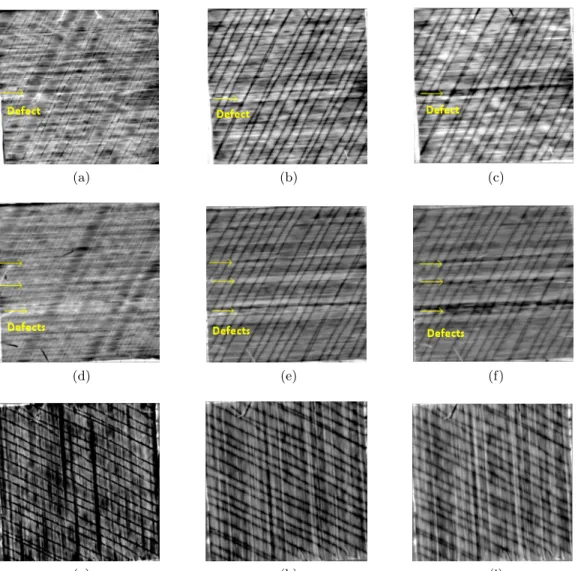
3.11 Thermographic results of PW-01 and US-03 using the flash/halogen lamps set-ups and 55 fps: (a) PW-03: 0.9 mm, (b) PW-01: 1.65 mm, (c) PW-01: B-TSR (1st), (d) PW-01: PCT (EOF03), (e) US-03: 0.5 mm, (f) US-03: 0.9 mm, (g)
US-03: B-TSR (1st), (h) US-03: PCT (EOF03).. . . 29
3.12 (a) US-03: Phase-based LT (0.8 mm), (b) US-03: PCT (EOF04), (c) US-03:
twisted front photo, (d) US-03: twisted rear photo. . . 29
4.1 BFRP specimens (rear side): (a) 7.5 J, (b) 15 J, (c) 22.5 J. . . 31
4.2 Jute/hemp fiber hybrid laminates (rear side): (a) plate No. 1, (b) plate No. 2,
(c) plate No. 3. . . 32
4.3 SCB specimens (front side): (a) 5 J, (b) 10 J, (c) 20 J, (d) 30 J. . . 32
4.4 Optical excitation thermography set-ups: (a) schematic set-up for LT [4], (b) schematic set-up for PT (flashes) [4], (c) experimental set-up for LT/PT
(halo-gen lamps), (d) experimental set-up for PT (flashes). . . 33
4.5 VT set-up, (a) schematic set-up using lock-in signals [4], schematic set-up using
pulse signals [4], (c) experimental set-up.. . . 34
4.6 UT experimental set-up. . . 35
4.7 CW sub-THz imaging system in reflection mode: (a) experimental set-up, (b)
schematic set-up. . . 35 4.8 PT results of BFRP: (a) 7.5 J: 0.28 mm, (b) 15 J: 0.28 mm, (c) 22.5 J: 0.28 mm, (d) 7.5 J: 0.85 mm, (e) 15 J: 0.85 mm, (f) 22.5 J: 0.85 mm, (g) 7.5 J: 1 mm, (h) 15 J: 1 mm, (i) 22.5 J 1 mm, (j) 7.5 J: PCT (EOF03), (k) 15 J: PCT (EOF04), (l) 22.5 J: PCT (EOF03). . . 37 4.9 UT results of BFRP: (a) 7.5 J, (b) 15 J, (c) 22.5 J. . . 38
4.10 VT results BFRP: (a) 7.5 J: PCT (EOF06), (b) 15 J: PCT (EOF03), (c) 22.5
J: PCT (EOF02). . . 38
4.11 Front-side results of 15 J BFRP: (a) photo, (b) UT result, (c) CW sub-THz result, (d) intensity curve for sub-THz result, (e) phase: 0.28 mm, (f) phase:
0.85 mm, (g) phase: 1 mm, (h) PCT: EOF03. . . 39
4.12 IRT results of JHFP: (a) plate No.1: 0.44 mm, (b) plate No.2: 0.44 mm, (c) plate No.3: 0.44 mm, (d) plate No.1: 1.72 mm, (e) plate No.2: 1.72 mm, (f) plate No.3: 1.72 mm, (g) plate No.1: PT (PCT: EOF02), (h) plate No.2: PT (PCT: EOF03), (i) plate No.3: PT (PCT: EOF03), (j) plate No.1: VT (PCT:
EOF04), (k) plate No.2: VT (PCT: EOF04), (l) plate No.3: VT (PCT: EOF06). 40
4.13 IRT results of SCB: (a) 5 J: 1.65 mm, (b) 10 J: 1.65 mm, (c) 20 J: 1.65 mm, (d) 30 J: 1.65 mm, (e) 5 J: 1.94 mm, (f) 10 J: 1.94 mm, (g) 20 J: 1.94 mm, (h) 30 J: 1.94 mm, (i) 5 J: PT (PCT: EOF), (j) 10 J: PT (PCT: EOF), (k) 20 J: PT (PCT: EOF), (l) 30 J: PT (PCT: EOF), (m) 5 J: VT (PCT: EOF), (n) 10
4.14 Phase-based LT results of SCB: (a) 5 J: 0.95 mm, (b) 10 J: 0.95 mm, (c) 20 J: 0.95 mm, (d) 30 J: 0.95 mm, (e) 5 J: 1.9 mm, (f) 10 J: 1.9 mm, (g) 20 J: 1.9 mm, (h) 30 J: 1.9 mm, (i) 5 J: 4.25 mm, (j) 10 J: 4.25 mm, (k) 20 J: 4.25 mm,
(l) 30 J: 4.25 mm. . . 43
5.1 Photographs of the impact regions (rear side): (a) B, (b) C, (c) BCs, (d) BCa. 47 5.2 Optical excitation thermography configurations: (a) schematic set-up for PT using flashes, (b) schematic set-up for LT and PT using lamps, (c) experimental set-up for PT using flashes, (d) experimental set-up for LT and PT using lamps. 47 5.3 VT configuration, (a) schematic set-up, (b) experimental set-up. . . 48
5.4 PCT results of PT: (a) B: EOF 04, (b) C: EOF 04, (c) BCs: EOF 04, (d) BCa: EOF 04. . . 49
5.5 PCT results of VT: (a) B: EOF 03, (b) C: EOF 03, (c) BCs: EOF 04, (d) BCa: EOF 03. . . 49
5.6 PLST results: (a) B: Loading 01), (b) C: Loading 01, (c) BCs: Loading 01, (d) BCa: Loading 01, (e) B: Loading 02, (f) C: Loading 02, (g) BCs: Loading 02, (h) BCa: Loading 02, (i) B: Loading 03, (j) C: Loading 03, (k) BCs:Loading 03, (l) BCa: Loading 03. . . 50
5.7 PPT results: (a) B: 0.68 mm, (b) C: 1.05 mm, (c) BCs: 0.87 mm, (d) BCa: 0.87 mm, (e) B: 0.96 mm, (f) C: 1.48 mm, (g) BCs: 1.23 mm, (h) BCa: 1.23 mm, (i) B: 1.19 mm, (j) C: 1.84 mm, (k) BCs: 1.52 mm, (l) BCa: 1.52 mm. . . 52
5.8 LT results: (a) B: 2.15 mm, (b) C: 2.09 mm, (c) BCs: 2.75 mm, (d) BCa: 2.75 mm, (e) B: 3.05 mm, (f) C: 3.31 mm, (g) BCs: 3.88 mm, (h) BCa: 3.88 mm. . 53
5.9 CT slices: (a) B: 0.1 mm, (b) C: 0.1 mm, (c) BCs: 0.1 mm, (d) BCa: 0.1 mm, (e) B: 0.6 mm, (f) C: 0.5 mm, (g) BCs: 0.8 mm, (h) BCa: 0.8 mm, (i) B: 0.8 mm, (j) C: 1.7 mm, (k) BCs: 1.7 mm, (l) BCa: 1.7 mm, (m) B: 1 mm, (n) C: 3 mm, (o) BCs: 2.7 mm, (p) BCa: 2.7 mm, (q) B: 3.3 mm, (r) C: 3.3 mm, (s) BCs: 3.3 mm, (t), BCs: 3.3 mm. . . 54
6.1 Typical dry-core in a non-stitched CFRP T-Joint (microscopic inspection). . . 58
6.2 (a) The complete 3D fabrication model, (b) a high-resolution photography of the preform, (c) the procedure of a triangular-shaped noodle processing for T-joint insertion. . . 59
6.3 (a) The textile unit cell model (mm), (b) the single layer preform model. . . 60
6.4 The model geometrical relation. . . 60
6.5 (a) Complete stitched 3D T-joint sample, (b) front side of the sample. . . 61
6.6 Microscopic inspection results of T-joint CFRP (a) top-section, (b) cross-section. 62 6.7 UT results of T-joint CFRP (2.25 MHz) (a) pulsed-echo, (b) through-transmission, (c) color scale for signal amplitude percent. . . 63
6.8 (a) Classical PT set-up[4], (b) experimental set-up. . . 64
6.9 PT results of T-joint CFRP (a) first derivative, (b) second derivative. . . 64
6.10 (a) Classical VT set-up[4], (b) experimental set-up. . . 64
6.11 VT results of T-joint CFRP.. . . 65
6.12 (a) Classical LST set-up[5], (b) experimental set-up[6]. . . 65
6.13 (a) image prior to heating, (b) heating spot. . . 66
6.14 ST results of T-joint CFRP (locked-in method) (a) surface, (b) depth: 0.21 mm, (c) depth: 0.65 mm . . . 66
6.15 (a) Micro-laser line thermography experimental set-up, (b) laser spot to laser
line. . . 67
6.16 The x-ray tomography results (a) surface, (b) depth: 90 µm, (c) depth: 0.18 mm. 68
6.17 The micro-laser line thermography results (a) cold image, (b) raw image with
contrast adjustment, (c) PCT. . . 69
6.18 The geometrical model. . . 71
6.19 (a) The micro-CT measurements (surface), (b) the corresponding model geo-metrical parameters, (c) the geogeo-metrical parameters of the porosities A and
B. . . 72
6.20 (a) surface temperature distribution (heating time: 0.5 s), (b) slice temperature distribution (heating time: 0.5 s), (c) surface temperature distribution from top
view. . . 73
6.21 Slice temperature distribution from top view when the heating time is 0.5 s: (a) surface, (b) depth: 50 µm, (c) depth: 0.1 mm, (d) depth: 0.2 mm, (e) depth:
0.5 mm. . . 74
6.22 Slice temperature distribution from side view: (a) heating time: 0.5 s, (b)
heating time: 1 s. . . 75
6.23 The simulation results after the corresponding image processing: (a) CIS, (b)
PCT. . . 75
6.24 Lock-in micro-LLT set-up: (a) experimental set-up, (b) schematic set-up. . . . 77
6.25 Micro-LST experimental set-up.. . . 78
6.26 Micro-CT slices (a) surface, (b) depth: 90 µm, (c) depth: 0.18 mm, (d) depth:
0.414 mm. . . 79
6.27 Micro-LLT results (a) pulse: 0.5 s, cold image, (b) lock-in: 5 Hz, PCT (EOF 8), (c) lock-in: 5 Hz, FT amplitude, (d) lock-in: 5 Hz, FT amplitude (defects marked) (e) lock-in: 1 Hz, FT amplitude, (f) lock-in: 1 Hz, FT amplitude
(defects marked) (g) lock-in: 5 Hz, FT phase, (h) lock-in: 1 Hz, FT phase. . . . 80
6.28 Micro-LST results (a) pulse: 0.5 s, cold image, (b) lock-in: 1 Hz, PCT (EOF
5), (c) lock-in: 1 Hz, FT amplitude, (d) lock-in: 1 Hz, FT phase. . . 81
6.29 Micro-VT experimental set-up. . . 82
6.30 Micro-VT results (a) pulse: 10 s, (b) pulse: 10 s (defects marked). . . 82
7.1 “James Abbott McNeill Whistler, Arrangement in Grey and Black, No. 1: Portrait of the Painter’s Mother, 1871, oil on canvas, 144.3 cm × 162.4 cm,
Musée d’Orsay, Paris". . . 88
7.2 The photographs of the paintings on canvas: (a) the canvas A, (b) the canvas B, (c) the textile support made from hemp and nettle, (d) the textile support
made from flax and juniper. . . 89
7.3 CW sub-THz imaging system: (a) schematic set-up in reflection mode, (b) schematic set-up in transmission mode, (c) experimental set-up in reflection
mode, (d) experimental set-up in transmission mode. . . 90
7.4 PT set-up using flash: (a) schematic set-up, (b) experimental set-up. . . 90
7.5 CW THz results: (a) painting on canvas A in reflection mode, (b) canvas A in transmission mode, (c) painting on canvas B in reflection mode, (d) canvas B
in transmission mode. . . 91
7.6 PCT results: (a) painting A: EOF 02, (b) painting A: EOF 03, (c) painting A:
7.7 PLST results: (a) painting A: Loading 01, (b) painting A: Loading 02, (c) painting A: Loading 03, (d) painting B: Loading 01, (e) painting B: Loading 02,
Abbreviations
B-TSR Basic thermographic signal reconstruction
BCa Basalt-carbon fiber hybrid composite with alternately stacked structure
BCs Basalt-carbon fiber hybrid composite with sandwich-like structure BFRP Basalt fiber reinforced polymer
CFRP Carbon fiber reinforced polymer
CH Culture heritage
CIS Cold image subtraction CT X-ray computed tomography CW Continuous wave
EOF Empirical Orthogonal Function FEA Finite element analysis
IRT Infrared thermography
JHFP Jute-hemp fiber hybrid polymer laminate LLT Laser line thermography
LT Lock-in thermography
Micro-CT X-ray micro-computed tomography
Micro-LLT Micro-laser line thermography Micro-LST Micro-laser spot thermography Micro-VT Micro-vibrothermography
NDT Nondestructive testing
PCT Principal component thermography PLST Partial least squares thermography
PPT Pulse phase thermography PT Pulsed thermography PW Plain weave
SCB Homogeneous Particleboards of Sugarcane Bagasse THz Terahertz
TW Twill weave
US Unidirectional stitched
UT Ultrasonic C-scan VT Vibrothermography
Texte de l’épigraphe
Acknowledgements
The last five years of my life has been filled with wonderful and challenging experiences for many reasons and I have a lot to be grateful for.
I would like to express my sincere gratitude and appreciation to my supervisor, Professor Xavier Maldague, for providing me guidance and encouragement. I appreciate the opportunity to work in such a professional but friendly environment.
I want to thank all the members of the Computer Vision and Systems Laboratory at Laval University. Specially I would like to mention Dr. Clemente Ibarra-Castanedo who helped me a lot during my Ph. D. and is always willing to help, listen and discuss new ideas; and Dr. Annette Schwerdtfeger who always so kindly helped me revising my texts.
I am very grateful for the collaboration with all team members of the CRIAQ COMP-501 project. Specially I would like to thank Prof. François Robitaille and Prof. Simon Joncas who helped me with the composite samples. Additionally the financial support of the industrial partners: Bell Helicopter (Canada) Inc., Bombardier Inc., Hutchinson Inc., Delastek Inc., Texonic Inc., CTT group through the following agencies: Natural Sciences and Engineering Research Council of Canada (NSERC), Consortium for Research and Innovation in Aerospace in Quebec (CRIAQ) and Canada Research Chair in Multipolar Infrared Vision (MiViM). I would also like to acknowledge the bilateral project supported by the governments of Québec and Bavaria, Ministère des Relations Internationales and Ministry of External Affairs. Spe-cially the support of Dr. Ulf Hassler from Fraunhofer EZRT (Germany).
I would also like to thank Dr. Stefano Sfarra from University of L’Aquila (Italy) and Marc Genest from National Research Council (NRC) Canada for their assistance.
I also want to extend my gratitude and appreciation to the thesis committee members for their time to read this thesis and for their valuable recommendations that contributed for the enrichment of the final version of this document.
Introduction
Background
Quality control (QC) is playing an increasingly important role for modern industrial produc-tion. This enhances the need of advanced image diagnostic techniques [7]. Image diagnostics has been applied in many sectors of QC, e.g., monitoring of electronic chips or dies in semi-conductor production lines, defect inspection during automatic manufacturing and damage detection of composite materials in the aerospace industry, etc [8; 9]. Image diagnostics in-cludes a wide group of analytical techniques used in science and industry to evaluate the properties of materials, components, or systems preventing potential damages after manufac-turing or in service [10;11]. During the manufacturing and applications of composite materials, besides employing advanced manufacturing techniques to raise the production rate, the uti-lization of reliable and cost-effective condition monitoring, fault diagnosis, non-destroctive testing (NDT), and structural health monitoring is very important [12;13;14]. In this direc-tion, the inspection of post-impact damages of industrial aerospace composite materials via image diagnostic techniques is becoming more and more common [15].
Infrared thermography (IRT) technique is based on the recording of images and is gaining increasing attention in the recent years due to its fast inspection rate, contactless nature, spatial resolution and acquisition rate improvements of infrared cameras. In addition, the de-velopment of advanced image processing techniques plays an important role in its exponential increment [16;17]. IRT can be used to assess and predict the structural integrity beneath the surface by measuring the distribution of infrared radiation and converting the measurements into a temperature scale [18]. Among the whole set of experimental set-ups, optical excitation thermography has been applied due to its ability to retrieve quantitative information concern-ing the defects. In addition, mechanical excitation thermography is also attractconcern-ing increasconcern-ing attention due to the powerful excitation approach.
The thesis is based on the image diagnosis and evaluation of different composite materials by IRT, ultrasonic C-scan (UT), X-ray computed tomography (CT) and continuous wave terahertz imaging (CW THz) for the comparative purpose. In addition, new IRT techniques are also proposed.
Research Objective
The main objective of the research is to evaluate different composite materials by IRT, UT, CT and CW THz for the comparative purpose. Advanced image processing technique will also contribute to the evaluation. New IRT techniques are also proposed to address the new issues in the field of NDT&E. Finally, a comprehensive and comparative analysis based on image diagnostics was conducted in view of potential industrial applications.
Organization
The thesis is organized into 7 chapters.
In Chapter 1, different NDT&E techniques are reviewed: 1) optical excitation thermography including PT and LT, 2) UT, 3) CT, 4) CW THz.
In Chapter 2, the common and recently developed data analyzing and image processing meth-ods are reviewed: 1) pulsed phase thermography (PPT), 2) partial least square thermography (PLST), 3) principal component thermography (PCT), 4) basic thermal signal reconstruction (B-TSR), 5) cold image subtraction (CIS).
In Chapter 3, optical excitation thermography was used to evaluate six carbon fiber dry preforms with different textile structures, thicknesses and defects. Comprehensive comparisons were conducted for: 1) providing the thermographic characteristics of different preforms; 2) summarizing the capability of image diagnostic/processing techniques; and 3) offering the most feasible monitoring modality for industrial manufacturing.
In Chapter 4, optical and mechanical excitation thermography were used to evaluate impacted mineral and vegetable fiber composites including basalt fiber reinforced polymer laminates (BFRP), jute/hemp fiber hybrid polymer laminates (JHFP), and homogeneous particleboards of sugarcane bagasse (SCB). In addition, UT and CW THz imaging were also carried out on the mineral fiber laminates. Finally, a comprehensive comparison of different techniques for natural fiber composites detection was conducted.
In Chapter 5, optical and mechanical excitation thermography were used to investigate basalt fiber reinforced polymer (BFRP), carbon fiber reinforced polymer (CFRP) and basalt-carbon fiber hybrid specimens subjected to impact loading. Of particular interest, two different hybrid structures including sandwich-like and intercalated stacking sequence were used. In particular, PT and LT were compared with x-ray computed tomography (CT) for validation.
In Chapter 6, a new laser line thermography (LLT) is presented. X-ray micro-computed tomography (micro-CT) was used to validate the infrared results. Then, a finite element analysis (FEA) is performed. The geometrical model needed for finite element dis-cretization was developed from micro-CT measurements. The model is validated for the experimental results. The same infrared image processing techniques were used for the
ex-perimental and simulation results for comparative purposes. In addition, a new micro-laser spot thermography (micro-LST) and micro-vibrothermography (micro-VT) were also proposed thanks to the use of micro-lens. Finally a comparison of micro-laser excitation thermography and micro-ultrasonic excitation thermography is conducted.
In Chapter 7, a CW THz (0.1 THz) imaging system was used to inspect paintings on canvas both in reflection and in transmission modes. In particular, two paintings were analyzed: in the first one, similar materials and painting execution of the original artwork were used, while in the second one, the canvas layer is slightly different. Flash thermography was used herein together with the THz method in order to observe the differences in results for the textile support materials. The canvas textiles can be considered as composite materials.
Chapter 1
A Review of NDT&E techniques
In this chapter, we will review the modern NDT&E techniques proposed in the literature.
1.1
Optical Excitation Thermography in this research
Optical excitation thermography includes pulsed thermography (PT) and lock-in thermogra-phy (LT) experimental set-ups among others.
In PT, photographic flashes or high-energy lamps are used to generate a heat pulse on the specimen surface. The heat transmits itself through the specimen, by diffusion, and then returns to the specimen surface. As time elapses, the surface temperature decreases uniformly for a specimen without internal flaws. On the contrary, subsurface discontinuities can be thought of as resistances to heat flow that change the diffusion rate and produce abnormal temperature patterns at the surface. If these patterns are large enough, then they can be detected with an IR camera and only a few mK as 4T is needed for the detection of thermal imprints using modern thermographic imaging equipment [4;19].
The Fourier equation for the propagation of a Dirac heat pulse in a semi-infinite isotropic solid by conduction is: T (z, t) = T0+ Q pkρcpπt e(− z 2 4αt) (1.1)
where, Q[J/m2]is the energy absorbed by the surface and T
0[K] is the initial temperature.
The Dirac heat pulse consists of periodic waves at all frequencies and amplitudes. A photo-graphic flash provides an approximately square-shaped heat pulse, which can be considered as a convenient approximation. Therefore, the signal can be decomposed by periodic waves at several frequencies. The shorter the pulse, the broader the range of frequencies.
LT, derived from photothermal radiometry, is also known as a modulated technique. In LT configuration, the absorption of modulated optical heating leads to a temperature modulation,
which transmits itself through the specimen as a thermal wave. When the thermal wave is reflected by the defect boundary, the superposition to the original thermal wave will lead to the transformation of the response signal amplitude and phase on the surface. These signals are simultaneously recorded by the IR camera. Photothermal radiometry is a raster point-by-point technique which requires a long acquisition time, especially for deep defects (low modulation frequencies). Sinusoidal waves are typically used in LT, which has the following advantages: 1) frequency and shape of the response are preserved, and 2) only the amplitude and phase delay of the wave may change [4;19].
Heat diffusion through a solid can be described by Fourier’s law of heat diffusion [20]: 52T − 1
α · ∂T
∂t = 0 (1.2)
where, α = k/ρcp[m2/s] is the thermal diffusivity of the material, k[W/mK] is thermal
con-ductivity, ρ[kg/m3]is the density, and c
p[J/kgK]is the specific heat at constant pressure.
Fourier’s law for a periodic thermal wave propagating through a semi-infinite homogeneous material can be expressed as [21]:
T (z, t) = T0e(−z/µ)cos(
2π · z
λ − ωt) (1.3)
where, T0[◦C] is the initial temperature change, ω = 2πf[rad/s] is the modulation frequency,
f [Hz] is the frequency, λ[m] is the thermal wavelength: λ = 2πµ, and µ[m] is the thermal diffusion length, which determines the rate of decay of the thermal wave as it penetrates through a material: µ = r 2 · α ω = r α π · f (1.4)
The amplitude and the phase delay can be calculated from the Fourier transform as detailed in section 2.1.
1.2
Mechanical Excitation Thermography
Vibrothermography (VT) uses mechanical waves to stimulate internal defects without heating the surface as in optical excitation thermography. Photothermal radiometry can be considered as the predecessor of optical thermography; VT should be the successor of optoacoustics or photoacoustics phenomena in which microphones or piezoceramics in contact with the specimen and a lock-in amplifier were used to detect the thermal wave signature from a defect. In VT, ultrasonic waves travel through a specimen, in which an internal defect results in a complex combination of absorption, scattering, beam spreading and dispersion of the waves. The waves generate heat which subsequently travels by conduction in all directions [22]. An IR camera faces the surfaces of the specimen to capture the defect signature [4].
1.3
Ultrasonic C-scan (UT)
Ultrasonic C-scan is a well-established NDT method which has the ability to detect flaws in either the partial or entire thickness of the materials[23]. It has been widely used to detect flaws in metals[24]. It is also increasingly used to detect composites due to its flexibility and convenience.
It is a challenge to detect thick 3D CFRP using ultrasonic c-scan due to its complex internal structure. The complex internal structure can cause attenuation and scattering of ultra-sonic beams[25]. Ultrasonic c-scan has been widely used to detect voids and laminates in composites[26].
1.4
X-ray Computed Tomography (CT)
The division between what is considered ’conventional’ computed tomography and ’micro-tomography’ is an arbitrary one, but generally the term micro-tomography is used to refer to results obtained with at least 50-100 µm spatial resolution [27]. CT has become a familiar technique. Recently it is also increasingly gaining popularity as an accessible laboratory technique for NDT of materials and components, especially due to the recent appearance of several commercial systems. Such instruments offer the potential for the widespread use of micro-CT as a tool for characterization of damage in composite materials [28].
Application of micro-CT to composite materials was concentrated on metal-matrix and ceramic-matrix composites in the past. The spatial scale of features in these materials including fiber location and waviness [29], fiber breakage [30], local porosity and density [31], void volume [32], fatigue crack growth [33], etc. are accessible to micro-CT. However, recently some studies on polymer matrix composites have also been reported. In 2000, impact damage including fiber fracture and delamination in T300/914 carbon fiber/epoxy laminates was characterized [34]. In 2002, impact damage in an epoxy/E-glass composite was also measured [35]. In 2004, micro-CT was used to determine internal structure in a polymer foam reinforced with short fibers [36]. In 2005, a study was undertaken to assess the capabilities and limitations of micro-CT for fiber-reinforced polymer-matrix composites, where different specimens with a variety of damage types, geometries and dimensions were investigated to assess the effect of the system resolution on the ability to determine the internal geometry of flaws including delamination, matrix crack, and especially micro-crack, which is a subject of critical interest in the study of fiber-reinforced polymer-matrix composite laminates [28]. In 2006, an evaluation of micro-CT was performed to determine the geometry of fiber bundles and voids in glass fiber reinforced polymers (GFRP). As a consequence, each fiber bundle and inter bundle voids can be observed separately [37].
1.5
Continuous Wave Terahertz Imaging (CW THz)
The electromagnetic waves range inherent to THz spectroscopy is located between 0.1 THz and 10 THz. THz wave generation is a challenge because the THz range is located at the boundary of electronics (based on the motion of electrons) and the photonics (based on the atomic transitions of electrons) modes of EM wave generation. However, the development of photonics and electronics in recent years has enabled the compact yet sophisticated THz imaging systems [38]. The principles of continuous wave (CW) imaging has been known for several decades [39;40]. Pulse imaging can provide depth, frequency-domain or time-domain information of the object, while CW imaging can only yield intensity data using a fixed frequency source and a single detector [41]. However, in THz imaging, a CW imaging system is compact, simple and relatively low-cost without a pump–probe system. Simultaneously, the complexity of the optics involved can be greatly reduced [42]. A recent THz time-domain system uses a shaker-technique to reduce measurement time, so the total observation time depends on scanning itself. Therefore, both pulse and CW THz systems can provide fast scanning. Regarding scientific research, simplicity is the main advantage of CW THz while the key advantage of pulse THz is flexibility, in which all the information is recorded within a single measurement to be processed in order to acquire the needed information for different applications. Since the frequency spectrum of CW THz is narrow, a large F -number Fresnel lens can be used to increase the resolution by focusing onto a spot [43].
In order to introduce the reader to the “result analysis" section it is important to describe the main physical concepts at the base of the THz method, as well as the experimental set up used to record the data. Usually, materials have different reflection and absorption coefficients for THz radiation, e.g., metals are better reflectors, polar liquids such as water are excellent absorbers, and anisotropic materials such as composites have variable reflectance relative to the fibre direction. The THz refractive indices and absorption coefficients are related to the material’s structure and properties. The Claausius-Mossotti equation (Eq. 1.5) [44] is usually used to calculate the refractive indices, which links the dielectric constant ε to the microscopic polarizability P , ε − 1 ε + 2 = 4π 3 NA ρ MP (1.5)
where NAis Avogadro’s number, ρ is the mass density, and M is the molecular weight.
The model developed by Schlömann [45] and Strom [46] is usually used to calculate the absorption coefficients. The model explains far-infrared absorption in amorphous materials in terms of disorder-induced coupling of radiation into the acoustic photon modes [47].
CW THz wave propagations in uniform solid materials is linear, and the transmission intensity can fit Beer’s Law very well. For instance, in case of wood inspection, it is known that spruce
absorption correlates with its density in the THz range, and this can be used for density mapping [48]. The derived CW THz absorption coefficient of various timbers can be obtained as follows [49]:
α
ρ ≈ 4.69 (1.6)
Chapter 2
Infrared Image Processing
In this chapter, we will review the infrared image processing techniques proposed in the liter-ature.
2.1
Pulsed Phase Thermography (PPT)
Discrete Fourier transform (DFT), or more precisely fast Fourier transform (FFT) on thermo-graphic data was first proposed by Maldague and Marinetti in 1996 [50]. DFT can be used to extract amplitude and phase information from LT and PT data. DFT can be written as [51]:
Fn= 4t N −1
X
k=0
T (k · 4t)exp(−j2πnk/N ) = Ren+ Imn (2.1)
where, j is the imaginary number (j2 = −1), n designates the frequency increment (n =
0, 1, . . . N), 4t is the sampling interval, Re and Im are the real and the imaginary parts of the transform, respectively.
Re and Im are used to estimate amplitude and phase [52]: An= p Re2 n+ Im2n (2.2) φn= tan−1( Imn Ren ) (2.3)
DFT can be used with any waveform and has the advantage of de-noising the signal. FFT can also be implemented instead of DFT for phase and amplitude transform due to its fast processing. The most important characteristic of phase and amplitude transform is that they provide the possibility to obtain quantitative results in a straightforward manner. A relationship exists between the depth z of a defect and the thermal diffusion length µ. Physico-mathematical expressions have been proposed, such as:
z = C1· µ = C1·
r α
where, fb is known as the blind frequency - the frequency at which a given defect has enough
(phase or amplitude) contrast to be detected, while C1 is calculated after a series of
experi-ments.
It has been observed that C1 ≈1 for amplitude transform [53], while reported values for phase
transform are in the range of 1.5 to 2 [53], with C1 = 1.82 typically adopted for similar cases
such as the present [54]. Therefore, for NDT applications, phase transform is more important than amplitude because it can retrieve the deeper information. The frequency components can be derived from the time spectra as follows:
fn=
n
N · 4t (2.5)
where, n designates the frequency increment (n = 0, 1, . . . N), 4t is the time step, and N is the total number of frames in the sequence.
Phase φn is particularly important because it is less affected than raw thermal data by
envi-ronmental reflections, emissivity variations, non-uniform heating, surface geometry, and ori-entation. These phase characteristics are very attractive not only for qualitative inspections but also for quantitative characterization of materials [19;4]. This technique is also known as pulse phase thermography (PPT) [50].
2.2
Partial Least Square Thermography (PLST)
Partial least square (PLS) methods relate the information present in two data tables that collect measurements on the same set of observations. PLS methods proceed by deriving latent variables which are optimal linear combinations of the variables of a data table. Indeed, one of the advantages of these techniques is the possibility of analyzing simultaneously two matrices X and Y , taking into account the relationship between each other. One of these matrices is necessarily the data matrix, the second one could be the time vector or a model matrix. After choosing a number of components c (usually, similar to the useful components in principal component analysis – PCA) PLS performs the simultaneous decomposition of both X and Y . Mathematically, PLS is expressed as follows:
X = T · PT + E (2.6)
Y = U · QT + F (2.7)
where, P and Q are defined as loadings, T is an orthogonal matrix defined as scores and E and F are residuals. If X ∈ Rnxs and Y ∈ Rnxm, then the loading P ∈ Rsxc, the loading
Q ∈ Rmxc and the score T ∈ Rnxc. In Equations 2.6and2.7, T (n × a) is known as the scores matrix and its elements are denoted by ta(a = 1, 2, . . . , A). The scores can be considered as
The matrices P (N × a) and Q(M × a) are called loadings (or coefficients) matrices and they describe how the variables in T relate to the original data matrices X and Y . Finally, the matrices E(n × N) and F (n × M) are called residuals matrices and they represent the noise or irrelevant variability in X and Y , respectively.
It can be noted in Equations 2.6 and 2.7 that the X-scores (T ) are predictors of Y and also model X, i.e., both Y and X are assumed to be, at least partly, modeled by the same latent variables. The scores are orthogonal and are estimated as linear combinations of the original variables xk with the coefficients, called weights, xka(a = 1, 2, . . . , A). Thus, the scores matrix
T is expressed by:
T = X · W (2.8)
Once the scores matrix T is obtained, the loadings matrices P and Q are estimated through the regression of X and Y onto T . Next, the residual matrices are found by subtracting the estimated versions of T PT and T QT from X and Y , respectively. Finally, the regression
coefficients for the model are obtained using Equation 2.8:
B = W · QT (2.9)
which yields the regression model:
Y = XB + F = XW QT + F (2.10)
The decomposition of the predictor X matrix is carried out using the nonlinear iterative partial least square (NIPALS) algorithm.
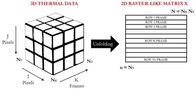
The application of PLRS to the square pulsed thermography (SPT) data is achieved by decom-posing the raw thermal data into multiple PLS components, each component being orthogonal to each other. Since each of the PLS components is characterized by its variance, it is pos-sible to identify via the PLS components different phenomena affecting the overall thermal regime. The thermal images obtained during the SPT inspection are typically arranged into a 3D matrix, whose x and y axes are represented, respectively, by i and j pixels, while the z axis corresponds to the k frame number. Nx and Ny correspond to the total number of pixels
along the x and y directions, while NT is the total number of frames (Fig. 2.1).
In order to perform the decomposition of the thermal data sequence into PLS components, it is firstly necessary to transform the 3D thermal data into a 2D raster-like matrix, as shown in Fig. 2.1. This process is known as unfolding. The unfolded X matrix (corresponding to the thermal sequence) has dimensions NT × Nx· Ny and physically represents NT observations
(or samples) of Nx· Ny variables (or measurements). On the other hand, the dimension of the
predicted matrix Y – defined by the observation time during which the thermal images were captured – is N × 1. More information regarding the PLST technique can be found in [55].
Figure 2.1: Schematic representation of the transformation of the 3D thermal data into a 2D raster-like matrix.
2.3
Principal Component Thermography (PCT)
Principal Component Analysis (PCA) used to process thermographic sequences to extract features and reduce redundancy by projecting the thermal response data onto a system of orthogonal components is known as PCT [56].
The PCA is a linear projection technique for converting a matrix A to a matrix of the lower dimension by projecting A onto a new set of principal axis. One simple approach to the PCA is to use Singular Value Decomposition (SVD). In general, a matrix A of the dimension M ×N (M > N) can be decomposed as [57]:
A = U RVT (2.11)
where U is the eigenvector matrix of the dimension M ×N, R is an N ×N diagonal matrix with positive or zero elements representing the singular values of matrix A, V T is the transpose of an N × N matrix.
For PCT, in order to apply the SVD to thermographic data, the 3D thermogram matrix representing time and spatial variations has to be reorganized as a 2D M × N matrix A [58; 2]. This can be done by rearranging the thermograms for every time as columns in A, as illustrated in Fig. 2.2a [2]. Under this configuration, the columns of U represent a set of orthogonal statistical modes known as Empirical Orthogonal Functions (EOFs) that describe the data spatial variations. On the other hand, the Principal Components (PCs), which represent time variations, are arranged row-wise in matrix V T . The resulting U matrix that provide spatial information can be rearranged as a 3D sequence as illustrated in Fig. 2.2b [2].
Figure 2.2: (a) Thermographic data rearrangement from a 3D sequence to a 2D A matrix in order to apply SVD, (b) rearrangement of 2D U matrix into a 3D matrix containing the EOFs [2].
Compared with FT that relying on prescribed basis functions (a set of sinusoidal basis func-tions), PCT method is an eigenvector based transform [57]. It is possible to achieve a compact representation for a complex signal by applying PCT. The first EOF will represent the most characteristic variability of the data; the second EOF will contain the second most important variability, and so on. Usually, 1000 thermogram sequence can be adequately represented with only 10 or less EOFs [58]. Beyond reducing redundancy, PCT is also proposed as a contrast enhancement approach [59].
2.4
Basic Thermographic Signal Reconstruction (B-TSR)
Thermographic Signal Reconstruction (TSR) [3] is widely used in commercial pulsed thermog-raphy systems. In TSR, a polynomial function is fit to each pixel time history to minimize temporal noise. Images created from the instantaneous logarithmic time derivatives of the fit function are typically viewed and analyzed, since the derivative images are much more sen-sitive to subsurface features than the original data sequence from the IR camera. Individual pixel time history derivatives can be evaluated quantitatively for automated evaluation or measurement of depth or thermal diffusivity. Once the polynomials have been calculated for each pixel, the coefficients may be archived instead of the original data sequence, resulting in significant degree of data compression.
It is important, though, to set the duration of pulse heating so as to accommodate the proper-ties of the sample. In particular, TSR is sensitive to transient events during cooling. Therefore, a long heating period and late acquisition may diminish the positive effects of TSR. Fig. 2.3
shows a typical use of TSR on a 8 plies CFRP specimen.
Figure 2.3: Typical use of TSR (model: 8 plies CFRP (0.0125” / ply)) [3]
The implementation of TSR that is used in industrial systems is based on patented and proprietary technology that has optimized specifically for performance with other components
in the system. In this study, we have used the basic form of TSR that has been reported in the literature, which we refer to as “B-TSR”. Our polynomial calculation is based on a standard Matlab polynomial fit. Results presented here using B-TSR do not necessarily represent the performance of commercial TSR systems.
2.5
Cold Image Subtraction (CIS)
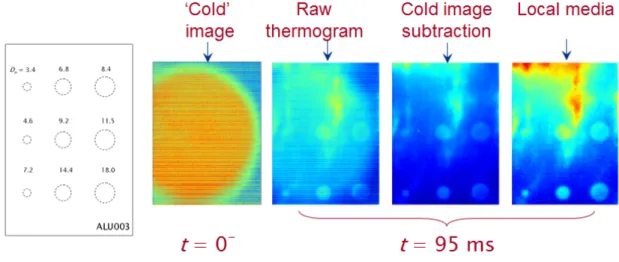
Cold image subtraction (CIS) is intended to reduce the effects of fixed artifacts in a ther-mographic sequence. For example, reflections from the environment such as residual heating coming from the lamps and even the reflection from the camera that appears during the acqui-sition. Since these artifacts are more or less constant during the whole acquisition, including before heating when the image is cold, this image or the average of several images can be subtracted before heating, so their effect can be reduced [60]. Figure 2.4 shows an example with an academic aluminum plate.
In Fig. 2.4, the cold image is affected by noise due to a non-uniform correction (NUC) which was badly performed. This happens when an old NUC is used. The noise can be seen in the raw sequence as well (the 2nd image in Fig. 2.4) although it is less evident since the temperature is higher.
Figure 2.4: An example with an academic aluminum plate to explain cold image subtraction.
Cold image subtraction can be considered as a pre-processing step to improve the quality of the sequence and then one can use more advanced algorithms such as phase pulse thermography, principal component thermography, etc.
Chapter 3
Image Diagnosis for Industrial Carbon
Fiber Dry Preform
3.1
Introduction
IRT, as an optical image diagnostic technique, has been used for composite materials [61;62]. However, IRT use for monitoring of dry preform during industrial manufacturing is poorly documented in the open literature.
CFRP, are preferred for aircraft component construction due to their excellent mechanical properties, e.g. high strength/stiffness and low densities [63; 64]. However, manufacturing costs remain an obstacle to wider use. Nowadays, CFRP are often manufactured using out-of-autoclave liquid molding (LM) processes, which provide flexibility and reduce cost. However, laying down thin reinforcement fabrics during the stacking process results in low reproducibil-ity. The use of advanced preforms, which are manufactured as assembled units, may alleviate this issue. Therefore, NDT is considered as a means of identifying defects in dry preforms during or after lay-down [14;13]. NDT conducted on dry preforms prior to resin infusion can greatly improve reproducibility and reduce rejection rates. Among NDT techniques, IRT is increasingly and particularly attractive [65;66].
In this work, pulsed and lock-in thermography were used to evaluate six carbon fiber dry preforms. Two of them are two-layered twill weave fabrics (thickness: ∼0.5 mm), one is a four-layered plain weave fabric (thickness: ∼1 mm), and the other three are stitched fabrics with two layers (thickness: ∼0.5 mm) and four layers (thickness: ∼1 mm). Flashes and halogen lamp set-ups were used, respectively. Quantitative analysis, which is important for NDT tech-niques, was conducted by phase transform. In addition, advanced image processing techniques including phase transform, CIS, B-TSR, PCT and PLST were used to process the thermo-graphic data for comparative purposes. In particular, PLST, one of the newest advanced post-processing techniques, was extensively applied. Finally, comprehensive comparisons were
conducted for: 1) providing the thermographic characteristics of different preforms; 2) sum-marizing the capability of image diagnosis/processing techniques; and 3) offering the most feasible monitoring modality for industrial manufacturing.
3.2
Carbon Fiber Dry Preforms
The specimens were made from 3 Texonic carbon fiber fabrics: a 215 g/m2 2×2 balanced twill
weave (TW), a 197 g/m2 balanced plain weave (PW), and a 285 g/m2 unidirectional stitched
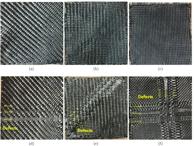
fabric (US). The fabrics were made from Toho Tenax HTS40 fibers. The TW and PW fabrics used 3K yarns while the US fabric used 12K yarns. For each fabric, a 100 mm × 100 mm specimen composed of 2 or 4 layers was prepared. Layers were assembled into preforms using Airtec2 spray adhesive, and each specimen was compacted under 4.6 KPa for 300 seconds. For the TW and PW specimens where the yarns extend along 2 orientations in each ply: 0/90◦ or ±45◦ shown in Fig. 3.1, the defects were fabricated by removing yarns. For the
(a) (b) (c)
(d) (e) (f)
Figure 3.1: Photographs of TW and PW specimens: (a) TW-01: front side, (b) TW-02: front side, (c) PW-01: front side, (d) TW-01: rear side, (e) TW-02: rear side, (f) PW-01: rear side.
to the orientation of yarns by cutting stitches to enable the removal of yarns, or by cutting yarns. The width/orientation of layers and defects are shown in Table 3.1. Measured sample thicknesses were ∼1 mm for PW-01/US-03, and ∼0.5 mm for the other TW/US specimens. The defects selected in this work are typical in manufacturing, and the corresponded NDT is poorly documented in the open literature.
(a) (b) (c)
(d) (e) (f)
Figure 3.2: Photographs of US specimens: (a) US-01: front side, (b) US-02: front side, (c) US-03: front side, (d) US-01: rear side, (e) US-02: rear side, (f) US-03: rear side.
Table 3.1: Orientation/width of layers and defects.
TW-01 TW-02 PW-01 US-01 US-02 US-03 Orientation of layer 0/90, 0/90 ±45, ±45 ±45, ±45, ±45, 0/90 0/90 90/90 90/90/90/90 Width & orientation of defect 1/2 yarn l ←→ 1 yarn ←→ % ←→ l ←→ l ←→ 2 yarn ←→ % ←→ l l ←→ 3 yarn ←→ % ←→ l
(a) (b)
(c) (d)
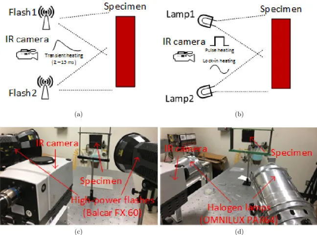
Figure 3.3: Optical excitation thermography set-ups: (a) schematic set-up for PT using flashes, (b) schematic set-up for PT and LT using lamps, (c) experimental set-up for PT using flashes, (d) experimental set-up for PT and LT using lamps.
3.3
Experimental Configurations
Fig. 3.3a and 3.3c show the schematic and experimental set-up for PT using photographic flashes, and two Balcar FX 60 (6.4 KJ each, 5 ms duration) photographic flashes were used in this set-up. Figs. 3.3b and 3.3d show the schematic and experimental set-up for PT and LT using halogen lamps, and two OMNLUX PAR64 (1000 W, 5 s duration) halogen lamps were used correspondingly. A mid-wave IR camera (FLIR Phoenix, InSb, 3 -5 µm, 640 × 512 pixels) was used to record the temperature profile. Three modalities were used: a) flashes set-up with 300 frames cooling time and 88 fps; b) flashes set-up with 10 s cooling time and 55 fps; and c) halogen lamps set-up with 15 s cooling time and 55 fps. In this work, RMF and CIS were performed prior to phase transform, B-TSR, PCT and PLST in PT; RMF was performed prior to Fourier transform and PCT in LT.
3.4
Experimental Measurement for Thermal Diffusivity
According to Eq. 2.4, the thermal diffusivity α is a parameter of particular interest for calculating the depth by phase transform. α can be obtained by either theoretical calculation or experimental measurement.
In the theoretical calculation method, α can be expressed as follows according to Eq. 1.1: α = k
ρcp (3.1)
where, cp[J/KgK] is the specific heat at constant pressure, ρ[Kg/m3] is the density, and
k[W/mK] is the thermal conductivity.
For composite materials, α can be calculated by [67;68;69]:
αcomposite= N
X
1
(Wf · αmaterial)N (3.2)
where, N is the number of constituent materials in the composite, and Wf is the weight
fraction material.
Eq. 3.2is linked to the fact that the α parameter is composed of physical quantities, but not composed of pseudo-physical quantities, as happens for the Cp parameter. Therefore, taking
into account the Buckingham theorem, it is possible to sum each layer for its volume fraction and mass fraction, respectively. This enables the obtaining of the final α and volume.
For carbon fiber dry preforms, the properties of both carbon fiber and air properties should both be considered. However, the weight fraction of air is difficult to quantify because of uncertainty over sample thickness. Therefore, an experimental measurement for α is more reasonable in this case.
In the experimental measurement method, the thermal diffusivity can be determined by ex-posing a sample of the material to a high-intensity, short duration heat pulse in the front face while recording the temperature evolution from the rear face. This approach was origi-nally proposed by Parker [70], based on determination of the time of maximum surface. The diffusivity can be obtained using the known specimen thickness L:
α = 0.139 · L 2 t1 2 (3.3) where t1
2 is the time when the temperature reaches half the maximum value.
This technique was later refined using different time parameters. The resulting technique is called the partial times method, in which the following equations were introduced to estimate the diffusivity [71]: α = L 2 t5 6 [0.818 − 1.708 · ( t1 3 t5 6 ) + 0.885 · ( t1 3 t5 6 )2] (3.4)
α = L 2 t5 6 [0.954 − 1.581 · ( t1 2 t5 6 ) + 0.558 · ( t1 2 t5 6 )2] (3.5) α = L 2 t5 6 [1.131 − 1.222 · ( t2 3 t5 6 )] (3.6)
where, α[m2/s]is the thermal diffusivity, which corresponds to the mean value of the three
re-sults; L is the specimen thickness; t1
2, t
1 3 and t
5
6 correspond to the times when the temperature
is equal to 1/2, 1/3, and 5/6 of the maximum value, respectively.
Estimations from any of these equations provide similar results. Fig. 3.4a shows the
experi-(a) (b)
Figure 3.4: (a) Experimental measurement set-up, (b) an example for the α calculation.
mental measurement modality using the flashes set-up, and Fig. 3.4b shows an example for the calculation of the mean value α. The same IR camera and flashes were used to record the temperature profile. Table 3.2 shows the thermal diffusivity α obtained by theoretical
Table 3.2: Thermal diffusivity by theoretical calculation and experimental measurement. Specimen Theoretical calculation Experimental measurement Thermal diffusivity α [10−7m2/s] TW/PW 1.85 ∼1.6
US 1.85 ∼0.5
calculation without considering air, and experimental measurements, respectively. In the the-oretical calculation, the following carbon fiber properties were used: cp = 1296 J/KgK, ρ =
1790 Kg/m3, k =0.43 W/mK [72]. In the measurements, the TW and PW specimens showed
similar thermal diffusivity, and the US specimens showed a similar value among themselves, but different values to TW and PW specimens. Therefore, mean value calculation were per-formed for the TW/PW and US specimens, respectively. This discrepancy may result from differences in air and carbon fiber value fraction difference, which is difficult to express in theoretical calculations in the case of dry preforms.
The measurement method cannot function properly when the specimen is thick, as heat cannot transfer throughout the specimen. In addition, the measurement is an approximate calculation, in which the specimen thickness plays an important role according to Eqs. 3.4-3.6. However, the measurement method is more appropriate than the theoretical calculation in this case due to the lack of information on the air volume fraction. Table3.3shows the calculated detection depth z according to the measured thermal diffusivity α and the modulated frequency fb used
in this work.
Table 3.3: Relationship between modulated frequency fb and detection depth z.
Modulated frequency fb[Hz] 2,9 1.1 0.65 0.35 0.2 0.08 0.065
Depth z[mm] TW/PWUS 0.25 0.40.15 / 0.50.3 0.4/ 0.90.5 0.8/ 1.650.9
3.5
Experimental Results and Analysis
Fig. 3.5shows the phase transform results for the TW and PW specimens. The flashes set-up and 88 fps was used with a cooling time of 300 frames. Images from depths of 0.25 mm (2.9 Hz), 0.4 mm (1.1 Hz) and 0.5 mm (0.65 Hz) were obtained. Defects in the two-layered TW specimens were detected at a depth of 0.4 mm as shown in Figs. 3.5band 3.5e, and they can be seen more clearly at a depth of 0.5 mm (Figs. 3.5c and3.5f). No defects were detected at a depth of 0.24 mm (Figs. 3.5a and 3.5d) since there were no defects located at this depth. Defects were detected with increasingly clear features along with depth. Defects in the four-layered specimen PW-01 (Figs. 3.5g, 3.5h and 3.5i) were not detected as they are located deeper than 0.5 mm.
Fig. 3.6 shows B-TSR and PCT results for TW and PW specimens using the flashes set-up and 88 fps. In B-TSR, the 1st derivative results are clearer. For the four-layered PW specimen, defects were detected by B-TSR and PCT, as shown in Fig. 3.6gand3.6i. PCT showed clearer results than phase transform, but the lack of quantitative analysis is a significant disadvantage. PLST can also provide additional results along with depth, as shown in Fig. 3.7. In PLST, 1st loading results are nearer to the surface than 2nd loading results, which are shallower than 3rd loading results. Similar to phase transform, defects were also detected with increasingly clear features along with depth. Again, defects in the four-layered specimen PW-01 were not detected. Although phase transform shows clearer results, PLST needs less processing time. However, PLST can only provide qualitative depth information, which is also a disadvantage compared with phase transform.
Fig. 3.8 shows phase transform results for US specimens obtained by the same modality as used for results shown in Fig. 3.5. Images at depths of 0.15 mm (2.9 Hz), 0.3 mm (0.65 Hz) and 0.4 mm (0.35 Hz) were obtained. The defects in the two-layered US specimens were detected
(a) (b) (c)
(d) (e) (f)
(g) (h) (i)
Figure 3.5: Phase transform results of TW/PW specimens using the flashes set-up and 88 fps: (a) TW-01: 0.25 mm, (b) TW-01: 0.4 mm, (c) TW-01: 0.5 mm, (d) TW-02: 0.25 mm, (e) TW-02: 0.4 mm, (f) TW-02: 0.5 mm, (g) PW-01: 0.25 mm, (h) PW-01: 0.4 mm, (i) PW-01: 0.5 mm.
in Figs. 3.8a - 3.8f, and they are increasingly clear as the depth increases. This observation concurs with the theoretical prediction because defects in the two-layered US specimens were fabricated from the middle depth approximately. Defects in the four-layered specimen US-03 (Figs. 3.8g,3.8h and 3.8i) were not detected because they are located much deeper than 0.4 mm. Compared with TW/PW resutls, defects in US specimens can be detected at shallower depths due to the simpler structures of the preforms. However, detection at deeper depths is more difficult than with TW and PW specimens due to the lower thermal diffusivity value. Figs. 3.9and3.10show B-TSR, PLST and PCT results for US specimens obtained using the flashes set-up and 88 fps. Defects in the four-layered specimen US-03 were not detected due to
(a) (b) (c)
(d) (e) (f)
(g) (h) (i)
Figure 3.6: B-TSR and PCT results of TW/PW specimens using the flashes set-up and 88 fps: (a) TW-01: B-TSR (1st), (b) TW-01: B-TSR (2nd), (c) TW-01: PCT (EOF03), (d) TW-02: B-TSR (1st), (e) TW-02: B-TSR (2nd), (f) TW-02: PCT (EOF03), (g) PW-01: B-TSR (1st), (h) PW-01: B-TSR (2nd), (i) PW-01: PCT (EOF01).
the lower thermal diffusivity value. Similarly, PLST results are not as clear as those obtained with the other techniques. However, PLST requires less processing time and it can provide qualitative depth information.
Fig. 3.11shows thermographic results for PW-01 and US-03 obtained with the flashes/halogen lamps set-ups and 55 fps. The cooling times were 10 and 15 s for the flashes/halogen lamps set-ups, respectively. For PW-01, the depths of 0.9 mm (0.2 Hz) and 1.65 mm (0.065 Hz) were investigated using the flashes/halogen lamps set-ups, respectively. For US-03, the depths of 0.5 mm (0.2 Hz) and 0.9 mm (0.065 Hz) were investigated correspondingly. Defects in PW-01
(a) (b) (c)
(d) (e) (f)
(g) (h) (i)
Figure 3.7: PLST results of TW/PW specimens using the flashes set-up and 88 fps: (a) TW-01: 1st loading, (b) TW-TW-01: 2nd loading, (c) TW-TW-01: 3rd loading, (d) TW-02: 1st loading, (e) TW-02: 2nd loading, (f) TW-02: 3rd loading, (g) PW-01: 1st loading, (h) PW-01: 2nd loading, (i) PW-01: 3rd loading.
were detected more clearly at a depth of 0.9 mm as shown in Fig. 3.11a, and they disappeared at a depth of 1.65 mm (Fig. 3.11b) because this is beyond the depths which can be successfully investigated in this specimen. Defects in US-03 were not detected at a depth of 0.5 mm (Fig.
3.11e), and a defect was detected at a depth of 0.9 mm (Fig. 3.11f), which coincides with the theoretical estimation. B-TSR and PCT show clearer results for both specimens. Detection in sample US-03 is more difficult than it is in the same-thickness PW-01, which may be due to its higher density as discussed in section 3.2. A possible solution is to increase the heat power by LT, which was also done in order to obtain additional information. The phase-based result at a depth of 0.8 mm (0.08 Hz and 3 periods) is shown in Fig. 3.12a, and the PCT result is shown in Fig. 3.12b. Indeed, phase-based LT shows clearer results and additional
(a) (b) (c)
(d) (e) (f)
(g) (h) (i)
Figure 3.8: Phase transform results of US specimens using the flashes set-up and 88 fps: (a) US-01: 0.15 mm, (b) US-01: 0.3 mm, (c) US-01: 0.4 mm, (d) US-02: 0.15 mm, (e) US-02: 0.3 mm, (f) US-02: 0.4 mm, (g) US-03: 0.15 mm, (h) US-03: 0.3 mm, (i) US-03: 0.4 mm.
information compared with phase-based PT. However, the fabric was twisted (Fig. 3.12cand
3.12d) after 3 periods of heating because the thermoplastic stitch cannot sustain the higher thermal energy, which shows a great difference from composites. Therefore, PT is the more feasible solution for carbon fiber dry preforms inspection according to the previous analysis in this work.
3.6
Summary
Image diagnosis and characterization for carbon fiber dry preform was conducted and analyzed by optical excitation thermography in this chapter, which demonstrates feasible fast IRT-NDT modality for dry preforms inspection prior to resin infusion and manufacturing. The
(a) (b) (c)
(d) (e) (f)
(g) (h) (i)
Figure 3.9: B-TSR and PCT results of US specimens using the flashes set-up and 88 fps: (a) US-01: B-TSR (1st), (b) US-01: B-TSR (2nd), (c) US-01: PCT (EOF01), (d) US-02: B-TSR (1st), (e) US-02: B-TSR (2nd), (f) US-02: PCT (EOF01), (g) US-03: B-TSR (1st), (h) US-03: B-TSR (2nd), (i) US-03: PCT (EOF01).
air and carbon fiber weight fraction difference leads to a discrepancy in thermal diffusivity, which is difficult to bring to light using theoretical calculation. Therefore, an experimental measurement of the thermal diffusivity prior to inspection is needed in the case of dry preforms. For higher density specimens, deeper detection is more difficult and requires more energy than for lower density specimens due to greatly different thermal diffusivities of the constituent materials.
Table. 3.4shows the performance of different thermographic techniques for dry carbon fiber preform inspection (the comparison is based on the specimens used in this work). Overall, IRT can provide clear results by phase transform, B-TSR, PCT and PLST. Among these techniques, B-TSR and PCT show the clearest results. The lack of quantitative analysis is a
(a) (b) (c)
(d) (e) (f)
(g) (h) (i)
Figure 3.10: PLST results of US specimens using the flashes set-up and 88 fps: (a) US-01: 1st loading, (b) US-01: 3rd loading, (c) US-01: 5th loading, (d) US-02: 1st loading, (e) US-02: 3rd loading, (f) US-02: 5th loading, (g) US-03: 1st loading, (h) US-03: 3rd loading, (i) US-03: 5thUS loading.
Table 3.4: Performance of thermographic methods.
Defect identification ability B-TSR ≈ PCT > phase transform ≈ PLST Technical simplicity (less processing time) B-TSR ≈ PCT ≈ PLST > phase transform
Quantitative analysis Shallow-defect PT (phase)
1 ≈ B-TSR
Deep-defect PT (phase)2 ≈ B-TSR ≈ LT (phase) Qualitative depth information Shallow-defect PT (phase)
1 ≈ B-TSR ≈ PLST
Deep-defect PT (phase)2 ≈ B-TSR ≈ PLST ≈ LT (phase) PT (phase)1: flashes modality; PT (phase)2: halogen lamps modality;
disadvantage of PCT [73]. Phase transform can provide quantitative analysis and additional information, which is often important for a NDT technique. PLST can also show additional results as the depth increases, but not as clearly as phase transform. PLST can only provide qualitative depth information, but it needs less processing time than phase transform. The
(a) (b) (c) (d)
(e) (f) (g) (h)
Figure 3.11: Thermographic results of PW-01 and US-03 using the flash/halogen lamps set-ups and 55 fps: (a) PW-03: 0.9 mm, (b) PW-01: 1.65 mm, (c) PW-01: B-TSR (1st), (d) PW-01: PCT (EOF03), (e) US-03: 0.5 mm, (f) US-03: 0.9 mm, (g) US-03: B-TSR (1st), (h) US-03: PCT (EOF03).
(a) (b) (c) (d)
Figure 3.12: (a) US-03: Phase-based LT (0.8 mm), (b) US-03: PCT (EOF04), (c) US-03: twisted front photo, (d) US-03: twisted rear photo.
flashes modality can detect shallow-defects because it can reach higher frequency. On the contrary, the halogen lamps modality is better for deep-defects detection.
Differently from composites, dry preforms featuring thermoplastic stitches cannot sustain high energy heating so that LT is inappropriate in such a case. Although this may limit the maxi-mum detection depth, IRT is a more feasible technique for dry preforms inspection compared with CT, which are much more expensive and time-consuming [60; 74]. Of interest, B-TSR and PCT are more appropriate for fast detection. Therefore, the development of an automatic system for identifying defects in dry preforms based on infrared computer vision could be built for industrial applications [75;76].