Compressed sensing applied to modeshapes reconstruction

To cite this document: Morlier, Joseph and Bettebghor, Dimitri Compressed

sensing applied to modeshapes reconstruction. (2011) In: IMAC XXX

Conference and exposition on structural dynamics, 30 Jan – 02 Feb 2012,

Jacksonville, USA.

OATAO is an open access repository that collects the work of Toulouse researchers and

makes it freely available over the web where possible.

This is an author-deposited version published in:

http://oatao.univ-toulouse.fr/

Eprints ID: 5163

Any correspondence concerning this service should be sent to the repository

administrator:

staff-oatao@inp-toulouse.fr

Compressed sensing applied to modeshapes reconstruction

Joseph Morlier 1*_{, Dimitri Bettebghor} 2

1 _{Université de Toulouse, ICA, ISAE DMSM ,10 avenue edouard Belin 31005 Toulouse cedex 4, France}

2 _{Onera DTIM MS2M, 10 avenue Edouard Belin, Toulouse, France}

* _{Corresponding author, Email: joseph.morlier@isae.fr, Phone no: + (33) 5 61 33 81 31, Fax no: + (33) 5 61 33 83 30}

ABSTRACT

Modal analysis classicaly used signals that respect the Shannon/Nyquist theory. Compressive sampling (or Compressed Sampling, CS) is a recent development in digital signal processing that offers the potential of high resolution capture of physical signals from relatively few measurements, typically well below the number expected from the requirements of the

Shannon/Nyquist sampling theorem. This technique combines two key ideas: sparse representation through an informed

choice of linear basis for the class of signals under study; and incoherent (eg. pseudorandom) measurements of the signal to extract the maximum amount of information from the signal using a minimum amount of measurements. We propose one classical demonstration of CS in modal identification of a multi-harmonic impulse response function. Then one original application in modeshape reconstruction of a plate under vibration. Comparing classical

!

2 inversion and

!

1 optimization to

recover sparse spatial data randomly localized sensors on the plate demonstrates the superiority of

!

₁ reconstruction (RMSE).

1. Introduction

Compared to nondestructive testing (ultrasound techniques, analysis of magnetic fields, radiology, thermal methods) vibration-based analysis allows a mixed global/local analysis of the structure with the potential of being applied in situ (laser vibrometer, optical sensor, etc) [1,2]. Deciding on an optimal sensor placement and optimal frequency sampling is a common problem encountered in many engineering applications and is a critical issue in the construction and implementation of an effective Structural Health Monitoring system (SHM). As a first example we study the modeshape reconstruction from grid placement. It highlights the fact that mode shapes visualization is often biased due to spatial aliasing. On figure 1, we can see that 9 grid point measurement are not enough precise to reconstruct the (3,1) mode shape.

Plate length (cm) P la te w id th ( cm ) 20 40 60 80 100 20 40 60 80 100 0 0.2 0.4 0.6 0.8 1 Plate length (cm) P la te w id th ( cm ) 20 40 60 80 100 20 40 60 80 100 ₀ 0.1 0.2 0.3 0.4 0.5

Fig. 1. : (3,1) mode of vibrating plate plus regular grid distribution of sensors in white circles (a) and The cubic interpolation which shows a spatial aliasing in mode shape reconstruction (b). A regular grid of 9 sensors permits only to reconstruct the (1,1).

In a first paper [3] we use Monte Carlo approach to demonstrate the ability of Kriging method at high spatial density to reconstruct mode shape with accuracy using regular or random grid. In this paper we are not analyzing a problem of Sensor Placement Optimization (SPO), which aims at identifying the sensor layout that will optimize one or more of the probabilistic performance measures. A detailed literature about SPO can be found in [2,4]. We prefer to have a “signal processing” approach. According to well known theorem sampling theorem, Stubbs and Park [5] introduced this theorem for spatial data for avoiding well know problem called “aliasing”. Schulz et al. [6] address the issue of damage resolution as a function of spatial distribution of sensors. They show that damage can be located within a spatial resolution equal to the distance between sensors on a structure. Sazonov and Klinkhachorn have developed an optimal sampling theory [7]. This approach allows us to estimate high resolution modeshapes taking into account experimental noise and enables to evaluate even small damages. This method use the curvature mode shape properties to find relationship between optimal sampling data and Signal to Noise Ratio and have been adapted for wavelets approach by Morlier et al [8].

The first works combining acoustic measurement and parcimonious approach were presented last year at the French Congress of Acoustics [9,10]. The advanced mathematical techniques so-called Compressive Sensing (CS) benefit fields as diverse as sensors, signal processing, image compression etc ... CS is used to find some kind of underlying structure behind most of the analog signals on the condition that these signals are sparse [11,12,13]. It is then possible to acquire signal at lower sampling frequency, and therefore no longer verify the Shannon/Nyquist frequency.

2. Compressive sensing: learning by numerical examples

The least-squares solution to such problems is to minimize the

!

₀norm—that is, minimize the amount of energy in the system. This is usually simple mathematically (involving only a matrix multiplication by the pseudo-inverse of the basis sampled in). However, this leads to poor results for many practical applications, for which the unknown coefficients have nonzero energy. To enforce the sparsity constraint when solving for the underdetermined system of linear equations, one can minimize the number of nonzero components of the solution. The function counting the number of non-zero components of a vector was called the

!

₀norm by David Donoho. Candès. et. al. [11,12], proved that for many problems it is probable that the

!

₁norm is equivalent to the

!

₀ norm, in a technical sense: This equivalence result allows one to solve the

!

₁problem, which is easier than the

!

₀ problem. Finding the candidate with the smallest

!

₁ norm can be expressed relatively easily as a linear program, for which efficient solution methods already exist [14].

The traditional approach to data acquisition is based on the Shannon-Nyquist theorem: to acquire a signal with a bandwidth of size W must be sampled at a higher frequency 2W. The compressive sensing exploits the fact that many real signals can be expressed in a sparse way and the inconsistency between certain types of bases to reduce this number of samples. A vector S-sparse is a vector that has at most S nonzero components. Many natural signals, when expressed in a particular base, have a representation with many significant coefficients. Data compression exploits this fact by removing these low coefficients, which slightly reduces the signal quality. These real-world signals (e.g. sound, images, video) can be viewed as an n-dimensional vector. To acquire this signal, we consider a linear measurement model, in which we measure an m-n-dimensional vector b = Ax ∈ Rm _{for some m × n measurement matrix A (thus we measure the inner products of x with the rows of A). For}

instance, if we are measuring a time series in the frequency domain, A would be some sort of Fourier matrix. This leads to the following classical question in linear algebra :

How many measurements m do we need to make in order to recover the original signal x exactly from b? The classical theory of linear algebra is as follows:

• If there are at least as many measurements as unknowns (m ≥ n), and A has full rank, then the problem is determined or overdetermined, and one can easily solve

Ax = b

uniquely (e.g. by gaussian elimination).

• If there are fewer measurements than unknowns (m < n), then the problem is underdetermined even when A has full rank. Knowledge of

Ax = b

restricts x to an (affine) subspace of Rn_{, but does not determine x completely. However,}

if one has reason to believe that x is “small”, one can use the least squares solution :

x = argmin

x:Ax=b

x

_!

2

= A

*

(AA

*

)

!1

Compressed sensing is advantageous whenever signals are sparse in a known basis. So the advantage is obvious when measurements (or simulations) are expensive and mathematical inversion is cheap. Such situations can arise in imaging (e.g. the “single-pixel camera”), Sensor networks, MRI Astronomy etc…and modal analysis.

In fact, the above proof also shows how to reconstruct an S-sparse signal

x ! R

n from the measurements

b = Ax

. x is the unique sparsest solution to

Ax = b

. In other words,

x = argmin

x:Ax=b

x

_! 0 (1) where

x

_! 0

:=

x

i 0 i=1 n

!

=#{1 " i " n:xi # 0}

is the sparsity of x.

Unfortunately, in contrast to the

!

₂ minimisation problem (least-squares),

!

₀minimisation is computationally intractable (in fact, it is an NP-hard problem). In part, this is because

!

₀minimisation is not a convex optimisation problem. A simple, yet surprisingly effective, way to do so is

!

1 minimisation (or basis pursuit); thus, our guess x* for the problem

Ax = b

is

given by the formula :

x

!

= argmin

x:Ax=b

x

_!

1 (2)

This is a convex optimisation problem, However, the

!

₁norm is not differentiable and this prevents from using classical optimization algorithm from differentiable optimization (such as SQP,...). Nonetheless, this non-differentiable convex optimization problem can be transformed in a linear programming optimization problem

x

!

= argmin

_x,y"#n_{,y >0:Ax=b i=1}

y

i n

$

and then can be solved fairly quickly by linear programming methods. Note that compressed sensing has equivalent formulations in the statistical field of regression. Best subset regression methods for instence seek amongst all the predictors the best set that explain the best the outcome to be predicted. This equivalent to

!

₀ minimization. Several heuristics exist to solve it through for instance best forward and best backward subset selection. The same way

!

1 minimization has equivalent

in regression, these are for instance lasso or LAR (Least Angle Regression) techniques. A valuable reference on these specific regression techniques is [15]. The main assumption behind these statistical techniques, which is precisely the same underlying assumption for compressed sensing, is known in statistics as bet on sparsity.

In a recent paper [16], the authors use CS on accelerometer signals of vibration of a bridge. The interest is obvious when engineers try to analyse vibrations during a year, using hundreds of sensors (MEMS and wireless network). We can note that the choice of the basis (wavelets, Fourier) is crucial with this type of approaches. In aeronautic we have the same interest in continuous monitoring of structures over a long period (flutter detection).

We try to illustrate a basic application of CS in the next example (using Matlab code

!

1-Magic of the University of Caltech

[14]). Let’s take the example of an analog signal (ie Fs = 400Hz >> Nyquist frequency) to 4 frequency components 30, 60,

100 and 130 Hz. We will compare in figure 2 the reconstruction of the signal regularly sampled at Fs=150 Hz using

0 0.5 1 1.5 2 2.5 ï0.4 ï0.3 ï0.2 ï0.1 0 0.1 0.2 0.3 0.4 time (s) Displacement

f = analog blue, f2 sampled magenta, b = random green

(a) 0 50 100 150 200 ï3 ï2 ï1 0 1 2 3 4 frequency (Hz) c = idct(f), idct(f2) Spectrum Magnitude (b) Fig. 2. Analog signal (in blue), discretized signal (magenta) respecting Nyquist frequency (N points) and

randomized signals at low resolution (N/10) (a), and DCT spectrum comparison (b)

We see that the spectrum (DCT) has four resonances in the continuous signal, and 4 also in the digital signal but aliasing appears because Fs is too low: the time signal reconstruction will not be correct. When we solve this problem using Moore-Penrose pseudo inverse, we can note the appearance of noise in Figure 3b (whereas CS imposes zero coefficients).

It is then easy to compare the result of the spectrum reconstructed by

!

₂norm and the solution "magic" by using the

!

₁ norm given in figure 3.

0 50 100 150 200 ï2 ï1 0 1 2 3 4 x = l₁ solution, A*x = b frequency (Hz) Spectrum Magnitude (a) 0 50 100 150 200 −0.3 −0.2 −0.1 0 0.1 0.2 0.3 0.4 0.5 frequency (Hz) Spectrum Magnitude y = l 2 solution, A*y = b (b) Fig. 3. Comparison of DCT spectrum of reconstructed signals by

!

₁ inversion (a) and

!

₂ inversion (b) of

randomized signals. The

!

₂ inversion is not capable of good reconstruction (noise)

We shall then compare the reconstruction on zoomed time signal (Figure 4) : NRandom varies from N/5 to N/10, where N

is number of samples. We see that the

!

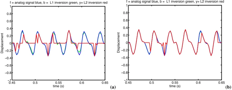
2 norm solutions and sampling the 'classic' is not correct with respect to the accuracy

0.45 0.5 0.55 0.6 0.65 ï1 ï0.8 ï0.6 ï0.4 ï0.2 0 0.2 0.4 0.6 0.8 1 time (s) Displacement

f = analog signal blue, b = L1 inversion green, y= L2 inversion red

(a) 0.45 0.5 0.55 0.6 0.65 ï1 ï0.8 ï0.6 ï0.4 ï0.2 0 0.2 0.4 0.6 0.8 1 time (s) Displacement

f = analog signal blue, b = L1 inversion green, y= L2 inversion red

(b) Fig. 4. Comparison of reconstructed signals by

!

₁inversion (green) for different sampling N/10 (a) and N/5: (b) of randomized signals. From the time domain (zoom) The

!

₂ inversion (red) is not capable of good reconstruction of the

continuous signal (blue) whereas

!

₁ optimization (green) is reliable even for low sampling.

Of course reconstructions

!

₂ and

!

₁inversion become better with increasing the number of observations. The current trend is to develop sampling acquisition cards for CS, but the requirements go beyond the technological limits of today's sensors.

3. Modeshapes reconstruction

When dealing with modeshapes reconstruction the principle is classicaly to make a regular grid of sensors. CS principles will permit to make sensor placement random. In numerical computation, surface interpolation functions create a continuous (or prediction) surface from sampled point values. The continuous surface representation of a raster dataset represents height, concentration, or magnitude. In Matlab, zi=griddata(x,y,z,xi,yi) fits a surface of the form z=f(x,y) to the data in the (usually) non uniformly-spaced vectors (x,y,z). Here we study empirically the feasibility of using. Shannon's sampling theorem is well known in 1D (time domain) but it also exists in 2D as demonstrate in the figure 5. Generally, the estimation accuracy will increase together with the sampling density.

(a) _(b)

Fig. 5.: In general artefacts are due to under-sampling or poor reconstruction: Temporal aliasing (Shannon’s theorem) (a), Spatial aliasing (b) due to limited spatial resolution and induce loss of details.

We propose to compare least square

!

₂inversion with CS method using randomly chosen sensors on the vibrating structures. A FEM modal analysis of a (Simply Supported) SSSS plate was done using following geometrical and material properties (length=width= 0.8m; height= 0.01m;E = 210e9 Pa; nu = 0.33; rho = 7700). We choose to illustrate the CS principle using few sensors and a well-chosen (physical) dictionary basis (Fourier Basis). In these numerical experiments, we used 8 sensors and chose a natural basis of the first 25 eigenmodes of simply supported rectangular plate. The

!

₂ norm minimization is computed through Moore-Penrose pseudo-inverse of the observation matrix A, while the

!

₁ norm minimization is performed through simplex method.

0 50 100 0 50 100 ï0.1 ï0.05 0

Real transverse displacement

ï0.1 ï0.05 0

Contour of real transverse displacement

0 20 40 60 80 100 0 20 40 60 80 100 ï0.1 ï0.05 0 0 50 100 0 50 100 ï0.1 ï0.05 0

L2 transverse displacement approximation

ï0.15 ï0.1 ï0.05 0

Contour of transverse displacement approximation

0 20 40 60 80 100 0 20 40 60 80 100 ï0.15 ï0.1 ï0.05 0 0 50 100 0 50 100 ï0.1 ï0.05 0 CS displacement approximation ï0.1415 ï0.0707 0

Contour of CS displacement approximation

0 20 40 60 80 100 0 20 40 60 80 100 ï0.1415 ï0.0707 0 0 50 100 0 50 100ï5 0 5

x 10ï3 Error for CS approximation

0 1 2 3 4

x 10ï3 Contour of error for CS approximation

0 20 40 60 80 100 0 20 40 60 80 100 0 1 2 3 4 x 10ï3 0 50 100 0 50 100 ï0.1 ï0.05 0

Real transverse displacement

ï0.1 ï0.05 0

Contour of real transverse displacement

0 20 40 60 80 100 0 20 40 60 80 100 ï0.1 ï0.05 0 0 50 100 0 50 100 ï0.1 ï0.05 0

L2 transverse displacement approximation

ï0.15 ï0.1 ï0.05 0

Contour of transverse displacement approximation

0 20 40 60 80 100 0 20 40 60 80 100 ï0.15 ï0.1 ï0.05 0 0 50 100 0 50 100 ï0.1 ï0.05 0 CS displacement approximation ï0.1415 ï0.0707 0

Contour of CS displacement approximation

0 20 40 60 80 100 0 20 40 60 80 100 ï0.1415 ï0.0707 0 0 50 100 0 50 100ï5 0 5

x 10ï3 Error for CS approximation

0 1 2 3 4

x 10ï3 Contour of error for CS approximation

0 20 40 60 80 100 0 20 40 60 80 100 0 1 2 3 4 x 10ï3 (a) (b)

Fig. 6. First modeshape reconstruction of a SSSS plate. The sensors are in red (randomly chosen) on the ‘continuous’ modeshape (a) one can see the

!

₂ inversion results on bottom. (b) We demonstrate the CS ability to reconstruct the

modeshape, on bottom one can see the error versus continuous modeshape (maximum error of 5E-3).

It should be noted whenever the dimension of x remains low, there is no substantial difference in terms computational burden between the two methods. However, for larger dimension (ranging from 100 for instance), the dimension of linear program, which is the double of the dimension of x, can lead to a prohibitive execution time. For such large problem decomposition-aggregation methods can help to save computational time. Indeed, the linear problem has a specific structure (often denote block-angular) that can be exploited through classical decomposition algorithm of large-scale linear programming (such as Benders decomposition or Dantwig-Wolfe decomposition).

Experimentaly modeshapes are commonly estimated from the residues obtained by curve fitting algorithm from set of FRFs [17]. This numerical study can be compared to experimental test where Laser Doppler Vibrometer can be moved automatically and so control the succession of acquisition for each point of the grid (regular or random). One can notice there are a variety of ways to derive a prediction for each location; each method is referred to as a model. With each model, there are different assumptions made of the data, and certain models are more applicable for specific data (for example, one model may account for local variation better than another). The existing methods of interpolation method can be found in [18,19]: Inverse Distance, Polynomial Regression, Kriging, Nearest Neighbour, Minimum Curvature, Radial Basis Function etc. Error due to sensor placement uncertainties can be defined by thrust regions (different radius depending of each sensor accuracy). This is not taken into account in this study but clearly affect the modeshape estimation.

4. Conclusion

We present an interesting approach for modal analysis using signals (1D, 2D) that do not respect the Shannon’s theorem. A simple multi harmonic vibration signal is proposed to illustrate the CS principles (

!

₁minimization). A more realistic example based on modeshape reconstruction has been done and the reconstruction appears to be enhanced by the use of CS method comparing to classical

!

₂ inversion. We also exhibit on the plate example (modal analysis) the crucial choice (physical) of dictionary basis (Fourier Basis). Future works will test the CS ability on more complex structures (thin-walled structure) using ‘optimized’ dictionary basis adapted for experimental modal analysis using random sensors placement.

References

[1] Doebling S. W., Farrar C. R., Prime M. B., and Shevitz D. W., Damage Identification and Health Monitoring of Structural and Mechanical Systems From Changes in Their Vibration Characteristics: A Literature Review, LANL Report LA-13070-MS, 1996.

[2] H. Sohn. C.R. Farrar, F. M. Hemez, D. D. Shunk, S. W. Stinemates, B. R. Nadler and J. J. Czarnecki, A Review of Structural Health Monitoring Literature form 1996-2001,LANL Report LA-13976-MS, 2004.

[3] Morlier, J., Chermain B. and Gourinat Y., Original statistical approach for the reliability in modal parameters estimation. (2009) In: MAC XXVII A Conference and Exposition on Structural Dynamics, 2009, Orlando.

[4] Guratzsch R.F., Sensor placement optimization under uncertainty for structural health monitoring of hot aerospace structures, PhD thesis, Vanderbilt University, 2007.

[5] Stubbs N., Park, S., and Sikorski Optimal sensor placement for mode shapes via Shannon's sampling theorem. Microcomputers in civil engineering , 11, 411-419, 1996.

[6] Schulz M.J., Naser A.S., Thyagarajan S.K., Mickens T., and Pai P.F. Structural Health Monitoring Using Frequency Response Functions and Sparse Measurements, Proceedings of the International Modal Analysis Conference, 760-766, 1998.

[7] Sazonov E., Klinkhachorn P., Optimal spatial sampling interval for damage detection by curvature or strain energy mode shapes, Journal of Sound and Vibration 285, 783-801, 2005.

[8] Morlier J., Bos F., Castera P., Diagnosis of a portal frame using advanced signal processing of laser vibrometer data, Journal of Sound and Vibration 297,2006, 420–431, 2006.

[9] Chardon G., Peillot A., Daudet L., and Ollivier F., Le “Compressed sensing” pour l’holographie acoustique de champ proche - I : Aspects algorithmiques et simulations, Actes du 10ème Congrès Français d’Acoustique, Lyon, France, 2010.

[10] Peillot A., Chardon G., Ollivier F., and Daudet L., Le “Compressed sensing” pour l’holographie acoustique de champ proche - II : Mise en oeuvre expérimentale, Actes du 10ème Congrès Français d’Acoustique, Lyon, France, 2010.

[11] E. J. Candès, J. Romberg and T. Tao. Stable signal recovery from incomplete and inaccurate measurements. Comm. Pure Appl. Math., 59 1207-1223, 2006.

[12] Donoho, D. L., Compressed Sensing, IEEE Transactions on Information Theory, V. 52(4), 1289–1306, 2006. [13] Candès, E.J., & Wakin, M.B., An Introduction To Compressive Sampling, IEEE Signal Processing Magazine, 2008. [14] L1-MAGIC is a collection of MATLAB routines: http://users.ece.gatech.edu/~justin/l1magic/

[15] Friedman J., Hastie T., Tibshirani R., The Elements of Statistical Learning, Springer, 2009.

[16] Yuequan Bao, James L. Beck, and Hui Li, Compressive sampling for accelerometer signals in structural health monitoring, Structural Health Monitoring, 2010.

[17] D. J. Ewins: Modal Testing: Theory, Practice and Application, 1995. [18] Funkhouser T.A., Computer Graphics Course COS 426, 1999.