THÈSE
THÈSE
En vue de l’obtention du
DOCTORAT DE L’UNIVERSITÉ DE TOULOUSE
Délivré par : l’Université Toulouse 3 Paul Sabatier (UT3 Paul Sabatier)
Présentée et soutenue le 5 Décembre 2016 par :
Alexandre Sauvé
Caractérisation des effets systématiques de l’instrument Planck/HFI, propagation et impact sur les données scientifiques
JURY
Peter VON BALLMOOS Professeur d’Université Président du Jury Anthony BANDAY Directeur de Recherche Co-directeur de thèse
François COUCHOT Directeur de Recherche Membre du Jury
Keith GRAINGE Professeur d’Université Rapporteur
Ludovic MONTIER Ingénieur de Recherche Directeur de thèse
Michel PIAT Maître de Conférences Membre du Jury
Isabelle RISTORCELLI Chargée de Recherche Membre du Jury
Louis RODRIGUEZ Ingénieur Rapporteur
École doctorale et spécialité :
SDU2E : Astrophysique, Sciences de l’Espace, Planétologie Unité de Recherche :
IRAP / CNRS (UMR 5277) Directeur(s) de Thèse :
Ludovic MONTIER et Anthony BANDAY Rapporteurs :
iii
Declaration of Authorship
I, Alexandre Sauvé, declare that this thesis titled, “Caractérisation des effets systématiques de l’instrument Planck/HFI, propagation et impact sur les données scientifiques” and the work presented in it are my own. I confirm that:
• This work was done wholly or mainly while in candidature for a research degree at this University.
• Where any part of this thesis has previously been submitted for a degree or any other qualification at this University or any other institution, this has been clearly stated. • Where I have consulted the published work of others, this is always clearly attributed. • Where I have quoted from the work of others, the source is always given. With the
exception of such quotations, this thesis is entirely my own work. • I have acknowledged all main sources of help.
• Where the thesis is based on work done by myself jointly with others, I have made clear exactly what was done by others and what I have contributed myself.
Signed: Date:
v
Résumé
Université Paul SabatierSciences de l’Univers de l’Environnement et de l’Espace Docteur en philosophie
Caractérisation des effets systématiques de l’instrument Planck/HFI, propagation et impact sur les données scientifiques
par Alexandre Sauvé
Planckest un satellite de l’ESA lancé en 2009, il représente la troisième génération
d’ob-servatoires spatiaux dans l’ère de la cosmologie de précision. Sa mission était de cartographier le fond diffus cosmologique (CMB) avec une extrême précision (∆T/T < 10−5). Le niveau
de précision requis nécessite un niveau de contrôle extrêmement élevé des effets systéma-tiques introduits par les instruments embarqués. Il se trouve qu’une combinaison inattendue d’éléments a conduit à une amplification de l’impact des effets de non linéarité introduits par le composant de numérisation des données scientifiques de l’instrument HFI, conduisant à l’introduction d’un des effets systématiques les plus difficiles à maîtriser. Ce manuscrit présente le travail qui a conduit à la caractérisation et à la correction de cette non-linéarité. Tout d’abord la modélisation de la réponse thermique complexe des détecteurs bolo-métriques sous intensité modulée est présentée. Puis la caractérisation de la réponse des détecteurs et de l’électronique de lecture est réalisée via l’utilisation du signal produit par l’impact des particules cosmiques sur les détecteurs. Dans un deuxième temps, les étapes menant à la caractérisation de précision des composants de numérisation sont détaillée. Pour pouvoir corriger l’effet de non-linéarité sur les données scientifiques, la chaîne complète de l’électronique de lecture est modélisée en prenant en compte la réponse des détecteurs sous intensité modulée et les effets non-linéaires du composant de numérisation avec le bruit. En plus de cela, il a fallu tenir compte du signal parasite complexe généré par le compresseur de l’étage de refroidissement cryogénique à 4 K, son inclusion dans la correction est détaillée. Ceci a mené à une correction qui a réduit l’impact de cet effet d’un ordre de grandeur sur le catalogue des données Planck de 2015. Finalement une étude est menée pour mesurer l’im-pact de cet effet de non-linéarité sur l’analyse scientifique de la Galaxie en polarisation et sur la cosmologie à travers le spectre de puissance angulaire du CMB. Une étude préliminaire est menée pour la détection de l’annihilation de nuages d’antimatière survivant à l’époque de la recombinaison en utilisant la carte d’effet Sunyaev-Zeldovich de Planck, et comment cette détection est affectée par la stratégie de scan de Planck.
vii
Abstract
Université Paul SabatierSciences de l’Univers de l’Environnement et de l’Espace Doctor of Philosophy
Caractérisation des effets systématiques de l’instrument Planck/HFI, propagation et impact sur les données scientifiques
by Alexandre Sauvé
Planck is an ESA spacecraft launched in 2009, it is the third generation of spatial
ob-servatory in the era of precision cosmology. Its mission goal was to map with an exquisite precision (∆T/T < 10−5) the Cosmic Microwave Background (CMB). The required level of
accuracy needs an unusually high level control of the systematic effects introduced by the on-board instruments. However, an unexpected conjunction of elements has enhanced the nonlinearity introduced by the chip performing the digitization of science data by the HFI instrument. It resulted in the most challenging systematic effect to deal with. It is presented here the work performed to characterize and correct for this nonlinear effect.
First a detailed modeling of the complex thermal response of the bolometer detectors under AC biasing is presented. The detector response is then further characterized by using the signal produced by cosmic particles. Second, the steps leading to the in-flight accurate characterization of the digitization chip are detailed. To correct for the nonlinear effect on science data, the full electronics readout chain response is modeled, taking into account the detector response under AC biasing and the nonlinear effect of the digitization chip with the noise. Furthermore, the complex parasitic signal originating from the 4 K cryogenic stage mechanical cooler has also to be taken into account. The provided correction has been applied with success to the HFI data 2015 release reducing the effect by an order of magnitude. Finally it is studied how the nonlinearity effect of the digitization component affects the galactic and cosmological scientific analysis through the angular power spectrum of the CMB. A preliminary study is performed for the detection of surviving antimatter clouds annihilating with matter at the epoch of recombination with the Planck map of Sunyaev-Zeldovich effect, and how it is affected by the scanning strategy of the spacecraft.
ix
Acknowledgements
Ce travaille de thèse s’est déroulé sur plus de trois ans, et avant toute autre chose je dois remercier mon fils qui du haut de ses sept ans a été extrêmement bienveillant à mon égard malgrès les très nombreuses heures que j’ai passé devant un écran au lieu de jouer avec lui.
Cette thèse est co-financée par le CNES et la société Noveltis, je tiens à les remercier et plus particulièrement Olivier Lamarle ainsi que Philippe Bru d’avoir accepté de me prendre sous leur aile.
Je remercie mon directeur de thèse Ludovic Montier de m’avoir offert l’opportunité de réaliser cette thèse ainsi que son énergie indéfectible pour débloquer tout les problèmes qui ont pu se présentér sur le chemin. Il a souffert avec beaucoup d’abnégation pour la relecture des deux articles que j’ai rédigé durant ces trois annés ainsi que ce manuscrit avec mon anglais approximatif qui n’aime pas les “s”. Mon co-directeur de thèse Anthony Banday a également été d’un grand soutien et a toujours su fournir des réponses précises et des conseils pertinents chaque fois que j’en avais besoin.
J’ai une pensée particulière pour François Couchot qui a porté à bout de bras l’équipe ADC pendant plusieurs années avec sa nonchalance et sa bonne humeur qui lui vont si bien. Il m’a donné de nombreux conseils et appris énormément, il a notamment porté à ma connaissance la méthode des Lagrange Multipliers qui a débouché sur la correction d’ADC utilisé pour les données Planck 2015. Mais surtout il m’a fait découvrir le P’tit Cahoua du Bd St-Marcel, ce qui n’a pas de prix!
Dans le travail sur les ADC j’ai également eu beaucoup de plaisir à échanger avec Guil-laume Patanchon, les discussions qu’on a eu étaient très animées et constructives.
Je tiens également à remercier toute l’équipe du café matinal (et bénévole) de l’IRAP sans qui rien de tout ceci n’aurait été possible!
The development of Planck has been supported by: ESA; CNES and CNRS/INSU-IN2P3-INP (France); ASI, CNR, and INAF (Italy); NASA and DoE (USA); STFC and UKSA (UK); CSIC, MICINN and JA (Spain); Tekes, AoF and CSC (Finland); DLR and MPG (Germany); CSA (Canada); DTU Space (Denmark); SER/SSO (Switzerland); RCN (Norway); SFI (Ireland); FCT/MCTES (Portugal); and PRACE (EU). A description of the
PlanckCollaboration and a list of its members, including the technical or scientific activities
in which they have been involved, can be found at http://www.rssd.esa.int/index.php? project=PLANCK&page=PlanckCollaboration.
xi
Contents
Declaration of Authorship iii
Résumé v Abstract vii Acknowledgements ix Introduction Générale 1 1 Introduction 7 1.1 Context . . . 7
1.1.1 History of the Universe . . . 7
1.1.2 The Cosmic Microwave Background . . . 7
Anisotropies . . . 8
The angular power spectrum . . . 9
1.1.3 Observational history of the CMB in brief . . . 11
1.2 The Planck spacecraft . . . 12
1.2.1 overview . . . 12
Mission goals . . . 12
History . . . 12
Characteristics of the HFI instrument . . . 13
1.2.2 Scanning strategy . . . 13
1.2.3 The cooling system . . . 14
1.2.4 HFI Systematics . . . 17
Major sources of systematics . . . 18
1.2.5 The Calibration and Performance Validation (CPV) phase . . . 19
1.2.6 The HFI Electronic Readout Chain . . . 19
Overview . . . 20
HFIdetectors biasing . . . 20
Amplification and balance of detectors signal . . . 20
Digitization by the ADC : the fast samples . . . 21
Signal summation . . . 21
Compression . . . 22
1.3 Data processing . . . 22
1.3.1 overview . . . 22
Time ordered data . . . 22
1.3.2 Production of HFI sky maps . . . 26
1.4 Polarization-Sensitive bolometers (PSB) of HFI . . . 27
1.5 Planck results . . . 28
1.5.1 Study of our Galaxy . . . 28
Polarization properties of dust grains . . . 28
1.5.2 The Sunyaev-Zeldovich (SZ) effect . . . 30 Clusters of galaxies . . . 31 Matter-Antimatter annihilation . . . 32 1.5.3 Cosmology . . . 33 1.6 Lessons learned . . . 34 I Readout Response 37 2 time transfer function analytical model 39 2.1 Context . . . 39
2.1.1 Definition of the time transfer function . . . 39
2.1.2 Characterization . . . 40
Thermal response model . . . 40
Calibration of the HFI thermal response . . . 40
Degeneracy with the scanning beam . . . 41
2.2 Discussion of the AC paper . . . 41
2.2.1 Motivations . . . 41
2.2.2 AC paper content . . . 43
2.2.3 Constraints for the LFER model . . . 43
2.3 Test of the analytical model against HFI data . . . 44
2.3.1 Fit setups . . . 44 2.3.2 Results . . . 45 Setup 1 . . . 45 Setup 2 . . . 45 Setup 3 . . . 45 2.4 Perspectives . . . 46
2.4.1 ADC nonlinearity correction . . . 46
2.4.2 Three thermal component model . . . 46
2.4.3 The disc form factor thermal model . . . 46
2.5 Conclusions . . . 49
3 Glitches exploitation 51 3.1 Introduction . . . 51
Glitches origin . . . 51
Characterization of the glitch families . . . 51
3.1.1 Relation with the time transfer function . . . 53
The continuous Finite Impulse Response (FIR) . . . 53
3.2 Building glitch templates . . . 56
3.2.1 Formalism . . . 56
Projection of glitches in Euclidean space . . . 56
Glitch selection . . . 57
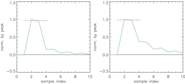
Glitch normalization . . . 58
Noise radius . . . 58
Visualization of the glitch cloud . . . 58
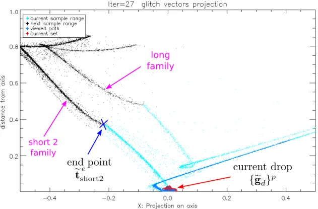
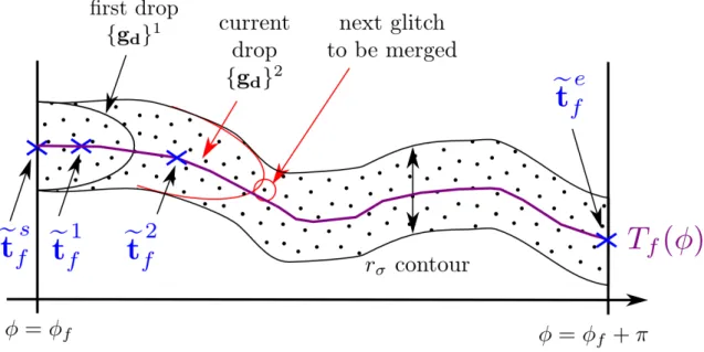
3.2.2 Glitch templates reconstruction with the capillarity method . . . 59
Localisation of starting point . . . 60
Path following . . . 61
3.2.3 Estimation of the continuous FIR . . . 62
Reconstruction of the continuous FIR . . . 62
xiii
3.3 Applications . . . 64
3.3.1 Validation of the the empirical time transfer function model . . . 64
3.3.2 Analysis of thermal properties of detectors . . . 65
3.3.3 High frequency transfer function constraints . . . 65
Motivation . . . 66
Model of the glitch FIR . . . 66
Results . . . 66
3.4 Perspectives . . . 68
3.5 Conclusions . . . 69
II ADC characterization and correction 71 4 ADC chip characterization 75 4.1 Historical overview of the ADC issue . . . 75
On-ground qualification : the back-door is open . . . 75
The variable gain mystery . . . 76
ADC nonlinearity evidence from fast samples histograms . . . 77
Dipole size compared to ADC nonlinear features . . . 77
The beginning of my contribution . . . 78
4.2 Understanding the ADC of HFI . . . 79
4.2.1 Basics of a Successive Approximation Register (SAR) ADC . . . 79
MSB and LSB . . . 79
Algorithm . . . 79
Architecture . . . 79
A non-ideal capacitive array . . . 80
4.2.2 ADC nonlinearity characterization in general . . . 80
Quantization noise . . . 81
Transfer function and Code Transition Points (CTP) . . . 82
Differential NonLinearity (DNL) . . . 82
Integral NonLinearity (INL) . . . 84
DNL estimation with ramp . . . 84
DNL estimation with Gaussian noise . . . 85
4.2.3 Target accuracy for INL characterization . . . 85
4.3 INL estimation from cold fast samples . . . 87
4.3.1 Slow thermal variations . . . 87
4.3.2 Estimation of INL with Gaussians . . . 87
4.3.3 Results of the INL estimation . . . 89
4.3.4 Fit of generic SAR nonlinearity model . . . 91
4.4 INL estimations from HFI electronics flight spare . . . 92
4.4.1 Experimental setup . . . 93
4.4.2 Data acquisition . . . 94
4.4.3 Estimation of INL from Setup B . . . 94
4.4.4 The 64-code periodic pattern . . . 95
4.4.5 Uncertainty estimation for the EOL sequence . . . 96
4.5 SPICE model approach . . . 97
4.5.1 Workplan . . . 97
4.5.2 DAC architecture of the 7809LPRP . . . 98
4.6 Cardiff full scale acquisition . . . 99
4.6.1 Acquisition setup . . . 99
4.7 INL estimation from in-flight warm data . . . 101
4.7.1 The EOL sequence . . . 101
EOL warmup . . . 101
HFIDPU reboot versus LFI requirements . . . 102
EOL sequence . . . 102
ADC scale coverage with ibias parameter . . . 104
Gaussian noise and channel gamp parameter . . . 104
4.7.2 INL estimation with maximum likelihood . . . 105
Signal model for EOL sequence . . . 105
Likelihood function . . . 106
Free parameters . . . 107
INL estimation method . . . 107
4.7.3 INL uncertainty . . . 108
4.8 Validation of a candidate INL . . . 109
4.8.1 The smooth histogram method . . . 110
4.8.2 The raw gain method . . . 110
ADC nonlinearity correction of fast samples . . . 111
Cold fast samples model of signal response . . . 111
Calculating the raw gain . . . 112
Overcoming the 4 K lines bias . . . 112
Stability of the raw gain over the mission . . . 113
4.9 Perspectives . . . 115
4.9.1 Avoiding ADC nonlinearity . . . 115
Increasing signal dynamic . . . 115
Using analog integration . . . 117
DPU correction . . . 117
4.9.2 New track for the INL estimation . . . 118
4.10 Conclusions . . . 118
5 Correction of science data 121 5.1 Principle . . . 121
5.2 Analog signal model . . . 122
5.2.1 Slow sky signal variations . . . 122
5.2.2 Signal Model . . . 123
5.2.3 The raw gain . . . 123
Estimation with a Principal Component Analysis (PCA) . . . 123
Inference of the relative error on the raw gain . . . 124
5.2.4 The raw constant . . . 125
Deglitching . . . 125
Characterization the raw constant parameter . . . 127
Per ring binning . . . 127
5.2.5 Iterative estimation of the parameters . . . 128
5.3 Digitization with noise . . . 129
5.3.1 Noise model . . . 129
5.3.2 summation of noisy fast samples . . . 130
5.3.3 Estimation of the fast samples noise RMS . . . 131
5.4 Science data transfer function . . . 132
5.4.1 Separation of modulation half periods . . . 132
5.4.2 Transfer function expression . . . 133
5.4.3 Correction of science data . . . 134
xv
Application to simulations at full mission scale . . . 135
5.5 Validation of the correction . . . 137
5.5.1 Formalism . . . 137
5.5.2 Production of PBRs with the 1D drizzling algorithm . . . 137
The 1D drizzling projection . . . 137
Filtering effect of the 1D drizzling . . . 138
Half parity PBRs . . . 139
5.5.3 The half parity gain observable . . . 139
5.5.4 The half parity sum observable . . . 140
5.5.5 Impact of ADC nonlinearity correction on bogopix gains . . . 141
5.5.6 Simulations . . . 142
Simulation setup . . . 142
Nulltest . . . 144
ADC nonlinearity effect validation . . . 146
Half parity observable characterization . . . 146
Frequency domain . . . 146
5.6 Conclusions . . . 147
6 4 K lines 149 6.1 Characterization of 4 K lines . . . 149
6.1.1 Origin . . . 149
6.1.2 Impact on ADC nonlinearity observables . . . 150
6.1.3 4 K lines on science data . . . 151
Spectral distribution on TOIs . . . 151
Estimation of 4 K lines with the 18 samples chunks method . . . 151
Drift over the mission . . . 153
Sub-ring variations . . . 155
Cross channel correlations . . . 159
Modulation by the sorption cooler bed switching . . . 159
6.1.4 4 K lines on fast samples . . . 162
The 4 K lines window problematic . . . 162
The CPV fast samples sequences . . . 164
Estimation of unfolded 4 K lines harmonics : the forrest . . . 164
Time domain drift over CPV 1 and CPV 2 . . . 167
Spectral drift over CPV 1 and CPV 2 . . . 167
6.2 Inclusion of 4 K lines in the ADC nonlinearity correction . . . 169
6.2.1 Updated analog signal model . . . 169
6.2.2 Updated science data transfer function . . . 169
6.2.3 Simulations . . . 170
Simulation of the 4 K lines effect on correction . . . 170
Susceptibility of ADC nonlinearity to 4 K lines harmonics . . . 171
6.3 Estimation of parameters for 2013 data release . . . 172
6.3.1 Breaking degeneracy with the half parity sum . . . 172
6.3.2 Using even modulation harmonics from CPV . . . 174
6.3.3 Parameters estimation using the Lagrange multipliers method . . . 175
6.3.4 2013 correction results . . . 176
Quantification of the improvement . . . 178
Analysis with the half parity 9-gain observable . . . 178
6.4 Alternative parameters estimation for 2015 correction . . . 181
6.4.1 Characterization of science data transfer function parameters . . . 181
Generation of transitions with folding constraints . . . 184
Analysis of the MCMCs . . . 186
Stability of the raw constant over the mission . . . 187
6.4.2 The global raw constant method . . . 189
Global raw constant model . . . 189
Estimation of the global raw constant parameter . . . 190
Results . . . 191
6.5 Conclusions and perspectives . . . 192
III Propagation of systematics on science 195 7 Propagation of ADC nonlinearity to science 197 7.1 ADC impact on Galactic polarization . . . 197
7.1.1 Simulation . . . 197
7.1.2 Degeneracy with the bandpass mismatch (BPM) effect . . . 199
7.2 ADC impact on CMB science . . . 200
7.2.1 Half-parity methodology . . . 201
Principle . . . 201
Production of HPD maps . . . 201
Characterization of the ADC effect on the T T spectrum with a simulation202 Multi-component Noise model for science data . . . 204
Comparison with half-ring difference (HRD) map . . . 206
7.2.2 Analysis of ADC nonlinearity impact on science . . . 207
Photometric calibration . . . 207
Impact on the T T spectrum . . . 209
7.2.3 Impact in polarization . . . 209
7.3 Conclusions . . . 211
8 Preliminary study for the detection of primordial matter-antimatter an-nihilation with Planck data 213 8.1 Introduction . . . 213
8.1.1 Context . . . 213
8.1.2 The Planck tSZ-map . . . 216
8.2 Characterization of the scanning strategy leakage . . . 216
8.2.1 Angular power spectrum split in the co/cross-scan directions . . . 216
8.2.2 Application of the co/cross-scan harmonic decomposition to the tSZ-map217 8.2.3 Characterization of the scanning strategy leakage with simulations . . 217
8.3 Conclusions and perspectives . . . 218
Conclusions et perspectives 223
Conclusions and perspectives 229
A Building the analytical response in frequency domain of AC biased
bolome-ters 235
B SPIE Astronomical Telescope + Instrumentation proceeding 263
xvii
D Orsay ground calibration datasets 285
E Schematics of the Cardif setup 287
F Sorption cooler schematic and sensors 289
G DMC objects Location 293
H Transfer function of the DPU summation 295
H.1 Parasitic wave description . . . 295 H.2 Raw samples integration effect . . . 296 H.3 Raw samples integration TF for 4K lines . . . 296
xix
List of Figures
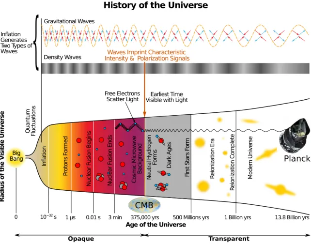
1.1 History of the Universe . . . 8
1.2 Spherical harmonics functions . . . 10
1.3 Angular power spectrum of the CMB . . . 10
1.4 The horn antenna used to make the first CMB detection . . . 11
1.5 Comparison of CMB results from COBE, WMAP and Planck . . . 12
1.6 Planck mission time-line . . . 13
1.7 Planck Scanning strategy . . . 14
1.8 Cutaway view of Planck, with the temperatures of key components in flight . 15 1.9 Thermal architecture of the HFI focal plane . . . 16
1.10 Thermal variations of the bolometer plate temperature over the mission . . . 17
1.11 Schematic of the HFI readout electronic chain . . . 19
1.12 Functional view of in-flight signal processing . . . 21
1.13 Example of raw science data TOI . . . 23
1.14 Example of Phased Binned Ring . . . 23
1.15 HFI 143 GHz intensity sky maps at different stages of processing . . . 24
1.16 Overview of the HFI data processing pipeline . . . 25
1.17 Example of an HFI PSB . . . 27
1.18 Planck full sky maps from the 9 frequency bands . . . 29
1.19 Polarized emission of foreground components . . . 30
1.20 All-sky view of the angle of polarization at 353 GHz . . . 31
1.21 Visualization of SZ effects for the cluster Abell 2319 . . . 32
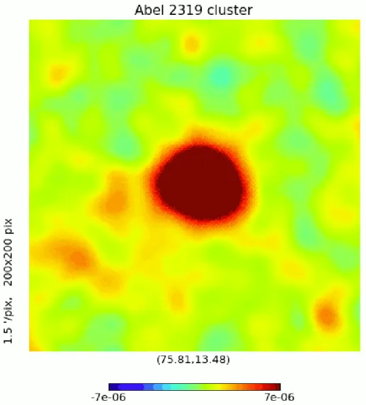
1.22 The cluster Abel 2319 as seen in the Planck y-map . . . 33
1.23 CMB intensity map at 50 resolution . . . 34
2.1 Thermal response of the time transfer function . . . 41
2.2 Scanning beam map . . . 42
2.3 Analytical model fit setup 1: data = raw gain only . . . 47
2.4 Analytical model fit setup 2: data = raw gain + TF . . . 47
2.5 Analytical model fit setup 3: data = TF only . . . 47
2.6 Thermal model with three components . . . 48
2.7 Thermal filtering profile for two 100 GHz channels . . . 48
2.8 Thermal dissipation with a disc model for the link to the heat sink . . . 49
3.1 Glitch rate versus SREM measurements and number of sun spots . . . 52
3.2 Examples of glitches on demodulated science data . . . 52
3.3 HFI bolometers annotated with glitch energy deposit locations . . . 54
3.4 Glitch families . . . 54
3.5 Simulation of glitch from energy deposit at different phases within the mod-ulation period . . . 55
3.6 Simulation of the continuous FIR . . . 56
3.7 Glitch normalization with pseudo energy . . . 57
3.8 Example of 2D projection of glitch cloud . . . 59
3.9 Example of glitches in start location configuration . . . 60
3.11 Examples of continuous FIR reconstructed with glitch dat . . . 63
3.12 Comparison of short glitch FIR with two early time transfer function model candidates . . . 64
3.13 Comparison of glitch families with the optical time transfer function . . . 65
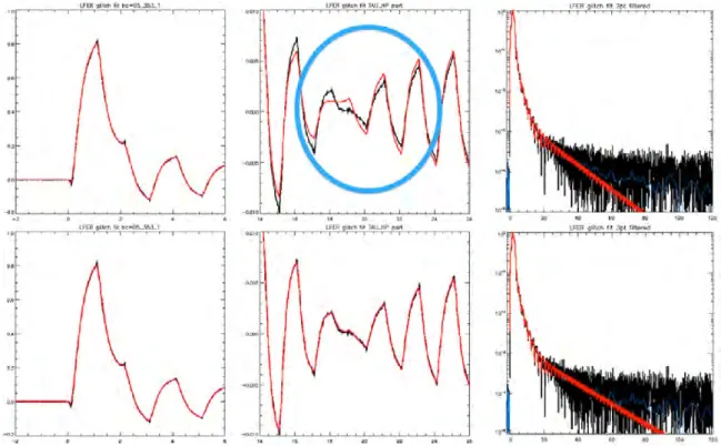
3.14 Fit residuals values for different free parameters selection of the LFER model 67 3.15 Example of fits of a short2 glitch with the LFER model . . . 67
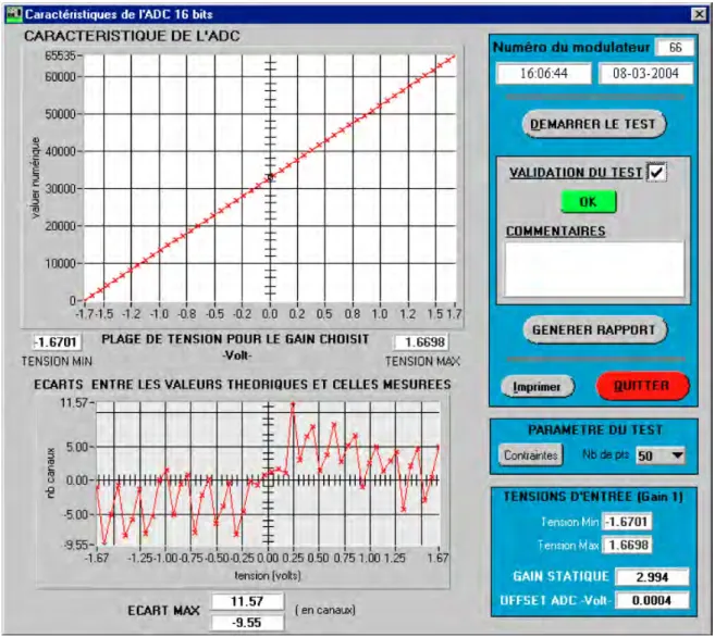
4.1 Example of on-ground qualification test for an HFI ADC . . . 76
4.2 Survey sky map differences before and after time variable gain correction . . 77
4.3 Histogram of the ADC output values over the HFI mission . . . 78
4.4 Example of SAR operation with a 4-bit ADC . . . 80
4.5 Simplified n-bit SAR ADC architecture. . . . 81
4.6 A 16-bit example of a capacitive DAC. . . 81
4.7 Example of a non ideal ADC transfer function . . . 83
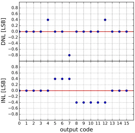
4.8 Example DNL and INL . . . 83
4.9 Normal CDF annotated with quantization step size . . . 86
4.10 DC level variations over the mission on a per ring basis . . . 87
4.11 Example of fast samples periods selection for local INL reconstruction . . . . 88
4.12 Example of INL and DNL built from cold fast samples . . . 89
4.13 Absolute error estimate for quantization step size built from cold fast samples 90 4.14 Generic SAR model fit results of the 11 first most significant bits for two channels. . . 92
4.15 Photo of the HFI electronics flight spare taken at IAS in February 2012 . . . 93
4.16 Histogram of fast samples for flight spare channel FS60 . . . 95
4.17 LCF drift on the INL for channel FS60 . . . 96
4.18 Resulting DNL and INL for FS60 after LCF component removal . . . 97
4.19 Resulting DNL and INL for FS60 after LCF component removal (Zoom) . . . 97
4.20 Visualization of the 64-code periodic pattern . . . 98
4.21 Correlation of DNL yielded by Setup A and B . . . 99
4.22 Diagram of the 7809LPRP DAC . . . 100
4.23 Fullscale INL estimated from Cardiff measurements . . . 101
4.24 INL with the 64-code pattern and jumps each 64 codes removed . . . 102
4.25 Temperature of the detectors plate during the first two month of EOL warmup103 4.26 Histogram of the fast samples acquired over the EOL sequence . . . 103
4.27 Variation of the REU temperature over the mission . . . 104
4.28 Signal shape for a warm detector . . . 105
4.29 Estimated INL for the ADC of the channel 00_100-1a . . . 109
4.30 Histogram of fast samples corrected for ADC nonlinearity . . . 111
4.31 Raw gains calculated with fast samples periods from different science data bins113 4.32 Effect of ADC nonlinearity correction on raw gain stability over the HFI mis-sion for channel 03_143-1a (unbiased) . . . 114
4.33 Estimation of ADC nonlinearity from raw gain consistency over HFI mission 116 4.34 Functional diagram of readout electronics with increased signal dynamic . . . 117
4.35 Functional diagram of readout electronics with analog integration . . . 117
4.36 Functional diagram of readout electronics with in-flight ADC correction . . . 118
5.1 Simplified model of the HFI readout electronics with ADC nonlinearity . . . 121
5.2 Typical signal dynamic of the solar dipole on channel 10_143-2a . . . 122
5.3 Principal Component Analysis outputs for channel 00_100-1a . . . 124
5.4 Example of raw gains estimated with a PCA . . . 125
xxi
5.6 Example of glitch on a fast samples period . . . 127
5.7 raw constant drift over the HFI mission for the channel 42-143-6 . . . 128
5.8 Effect of noise on the ADC transfer function . . . 130
5.9 PDF of the squared residuals for fast samples periods fit . . . 132
5.10 PDF of the squared residuals for fast samples periods compared with simulations133 5.11 Correction parameters shifted to the first fast samples integration index for channel 01_100-1b . . . 133
5.12 Science data transfer function for both modulation parities on channel 01_100-1b134 5.13 Simulation at fast samples level of the readout chain with nonlinear ADC . . 136
5.14 Simulation of ADC nonlinearity correction residuals for parity zero . . . 136
5.15 The 1D drizzling projection . . . 137
5.16 Transfer function modulus of the 1D drizzling in the HFI configuration . . . . 138
5.17 Example of PBRs produced with the 1D drizzling . . . 140
5.18 Correlation plot between PBRs produced from each modulation parity . . . . 141
5.19 ADC observable: the half parity gain relative difference . . . 142
5.20 Half parity gain observable for all channels . . . 143
5.21 ADC observable: the half parity sum standard deviation . . . 144
5.22 Bogopix gains . . . 144
5.23 Simulation of ADC nonlinearity effect over the full mission . . . 145
5.24 Simulation of ADC nonlinearity effect in frequency domain . . . 147
6.1 The 4K mechanical compressors, prior to integration to the spacecraft . . . . 150
6.2 Correlation plots between the 4 K lines level and ADC nonlinearity observables152 6.3 4 K lines on science data TOI spectra . . . 153
6.4 Difference between the 4 K lines removal by cutfreq and a manual version . 154 6.5 Estimation of 4 K lines with the 18 samples chunks method . . . 155
6.6 4 K lines drift throughout the mission . . . 155
6.7 4 K lines amplitude drift in time on science data for all channels . . . 156
6.8 4 K lines at sky circle time scale averaged on all channels . . . 157
6.9 4 K lines at sky circle time scale averaged on all channels . . . 157
6.10 DFT of 4 K lines amplitudes all over the mission at one minute time resolution158 6.11 4 K lines correlation matrices for full sky survey 1 . . . 160
6.12 4 K lines correlation matrices for full sky survey 2 . . . 160
6.13 4 K lines correlation matrices for survey 3 . . . 161
6.14 4 K lines correlation matrices for survey 4 . . . 161
6.15 Schematic of the LFI 20 K sorption cooler . . . 162
6.16 Comparison of sorption cooler helium pressure and 4 K lines variations . . . . 163
6.17 Estimated periodicity of the 4 K lines shortest modulation . . . 163
6.18 Example of contiguous fast samples periods from the CPV2 sequence . . . 165
6.19 Spectral distribution of the unfolded 4 K lines during the CPV 2 sequence . . 166
6.20 Spectral distribution of the unfolded 4 K lines for all channels grouped by belt during the CPV 2 sequence . . . 166
6.21 Reconstructed time domain 4 K lines periods for CPV 1 and CPV 2 . . . 168
6.22 Variation of the time domain unfolded 4 K lines period between CPV 1 and CPV 2 . . . 168
6.23 Spectral drift over CPV 1 and CPV 2 . . . 169
6.24 Simulation of 4 K lines impact on ADC nonlinearity using half parity gain observable . . . 171
6.25 Spectrum of ADC nonlinearity susceptibility Sg to unfolded 4 K lines . . . . 173
6.26 Even modulation harmonics templates from CPV . . . 174
6.28 Estimates of unfolded 4 K lines harmonics . . . 177 6.29 Removal of 4 K lines from the averaged fast samples period . . . 177 6.30 ADC nonlinearity observables for the Planck 2013 data release . . . 179 6.31 ADC nonlinearity 9-gain observables for the Planck 2013 data release . . . 180 6.32 Half parity 9-gain observables for all HFI detector channels (no correction) . 182 6.33 Half parity 9-gain observables for all HFI detector channels (2013 correction) 183 6.34 Schematic view of the folded vector complement for the transition . . . 185 6.36 Burn in period of the MCMC . . . 187 6.37 Likelihood of harmonic values with tight prior on amplitudes . . . 188 6.38 Likelihood of harmonics values with relaxed prior on amplitudes . . . 188 6.39 Likelihood with only 7 harmonics . . . 188 6.40 Consistency of half period sum residuals over the mission . . . 189 6.41 Consistency of the raw constant over the mission . . . 190 6.42 half parity sum of the global raw constant . . . 191 6.43 ADC nonlinearity residuals after correction with the global raw constant
pa-rameter set . . . 192 6.44 ADC nonlinearity observables calculated with the 2015 parameter set . . . . 193 7.1 Functional diagram for the simulation of ADC nonlinearity residuals in
polar-ization . . . 198 7.2 Simulation of polarization maps at 353 GHz . . . 198 7.3 Simulation of ADC nonlinearity residuals on polarization maps at 353 GHz . 199 7.4 Simulation of ADC nonlinearity effect on polarization fraction and angle at
353 GHz . . . 199 7.5 Dust leakage correction maps 353 GHz . . . 200 7.6 Half-parity difference map principle . . . 201 7.7 HPD maps before and after ADC nonlinearity correction . . . 202 7.8 TT power spectrum calculated with HPD maps . . . 203 7.9 TT power spectrum calculated with simulated HPD maps . . . 203 7.10 Simulation of the HPD noise spectrum at TOI level . . . 204 7.11 Functional diagram for the multi-component noise model of science data . . . 205 7.12 Validation of the multi-component noise model on science data TOI . . . 205 7.13 Comparison with the T T spectrum of the HRD map . . . 207 7.14 ADC nonlinearity error compared to the solar dipole amplitude . . . 208 7.15 Impact of ADC nonlinearity on the scientific analysis of the T T spectrum . . 209 7.17 TT EE and BB spectra of ADC nonlinearity residuals estimated from HPD
maps of 143 GHz channels . . . 212 8.1 Expected patterns for the interfaces between matter and antimatter . . . 214 8.2 Constraints on ABC domain size from gamma observations . . . 215 8.3 Planck map of the Compton parameter . . . 219 8.4 Leakage of the scanning strategy in the tSZ-map . . . 219 8.5 Spherical harmonics selection for co-scan / cross-scan directions . . . 220 8.6 Co/cross-scan angular power spectra of the tSZ-map . . . 220 8.7 Co/cross-scan harmonic decomposition in a small region of the tSZ-map . . . 221
xxiii
List of Tables
2.1 Results of the raw gain and 2015 time transfer function fit using the analyt-ical model on channel 00_100-1a. The time constant of the second thermal component is calculated with τ2ϕ = Gs02/C02 by extrapolation of the single
component formula. . . 45 3.1 Cases of free parameter considered . . . 66 3.2 . . . 68 4.3 gamp parameter . . . 105 6.1 dates of the fast samples CPV sequences . . . 164 6.2 Global raw constant parameter sets produced in 2015 . . . 191 G.1 DMC objects location for detectors channels. The bc label is meant to be
xxv
List of Abbreviations
ADC Analog to Digital Converter ADU Analog Digital Unit
CMB Cosmic Microwave Background CPV Calibration Performance Validation CTP Code Transition Point
DAC Digital to Analog Converter DFT Discrete Fourier Transform DNL Differential Non Linearity DPC Data Processing Center FPU Focal Plane Unit
HFI High Frequency Instrument INL Integral Non Linearity LFI Low Frequency Instrument LSB Least Significant Bit PAU Pre Amplifier Unit PLA Planck Legacy Archive
PSB Polarization Sensitive Bolometer PDF Probability Density Function REU Readout Electronic Unit RMS Root Mean Square SWB Spider Web Bolometer SZ Sunyaev Zeldovich (effect) TF Transfer Function
xxvii
List of Symbols
P power W (J s−1)
ω angular frequency rad
≡ equivalent to binary operator ' asymptotically equivalent binary operator ≈ is approximately binary operator ∝ is proportional to binary operator hxi average value of x unary operator
1
Introduction générale
Pour bien définir le fond du sujet qui nous intéresse commençons par un tour d’horizon de la théorie sur la formation de notre Univers qui décrit le mieux les observations. Selon la théorie de l’inflation, l’Univers a connu une période d’expansion très rapide après l’instant initial du Big Bang pendant ses premières 10−32s. Dans les instants qui ont suivi, la matière et
l’anti-matière se sont formées, leur annihilation réciproque a donné naissance à la la majeure partie des photons du fond diffus cosmologique (CMB), mais une légère asymétrie dans le rapport des deux en faveur de la matière a fait que cette dernière domine dans l’Univers moderne. Environ 380 000 ans après l’instant initial, l’expansion qui a suivi l’inflation a suffisamment refroidis le plasma dense et chaud de matière baryonique et de photons pour permettre la recombinaison des protons avec les électrons libres et former des atomes d’hydrogène ma-joritairement. C’est à cette époque qu’on appelle la recombinaison que le CMB est émis, ses photons n’étant plus soumis à la diffusion Compton sur les électrons libres ont pu se propager jusqu’à nous en ayant un minimum d’interactions avec la matière. La période qui a suivi s’appelle l’age de l’obscurité. C’est pendant ce temps que la matière a commencé à s’effondrer sur elle même à cause de l’instabilité gravitationnelle et que les premières grandes structures de l’Univers se sont formées. Par la suite la première lumière émise par les galaxies naissantes et la quasars a de nouveau ionisé l’hydrogène, c’est l’époque de la réionisation, ce qui a eu pour effet de diffuser à nouveau une fraction des photons du CMB à grande échelle angulaire sur les électrons de nouveau libres.
Le CMB se présente de nos jours comme une émission uniforme sur le ciel avec un spectre de corps noir à la température de 2.7255 K. Si on fait abstraction du dipôle solaire dû à l’ef-fet Doppler de notre vitesse relative dans le référentiel du CMB, apparaissent de petites variations de températures de l’ordre de ∆T = 1 × 10⁻⁵K, qu’on appelle les anisotropies.
Ces anisotropies qu’on qualifie de primaires sont principalement dues aux oscillations acous-tiques adiabaacous-tiques produites par la compétition entre la gravité et la pression des photons à l’époque où le CMB a été émis. Elles présentent une distribution caractéristique dans leurs amplitudes et leurs échelles angulaires qu’on mesure avec le spectre de puissance angulaire. Ce spectre de puissance angulaire est très bien décrit avec les six paramètres du modèle cosmologique ΛCDM (Cold Dark Matter) qui fournit une estimation précise de la densité de matière et d’énergie dans l’Univers mais nécessite l’introduction d’énergie sombre et de matière sombre n’interagissant pas avec la matière ordinaire. Une petite fraction des pho-tons du CMB sont polarisés par deux types de perturbations, les premières sont scalaires et proviennent des variations de densité de matière dues aux oscillations acoustiques, ce qui produit de la polarisation avec une orientation radiale ou circulaire qu’on appelle les modes-E en polarisation. Les secondes sont dues aux ondes gravitationnelles générées pendant l’infla-tion. Elles se manifestent également par des modes-E ainsi que par de la polarisation avec une orientation tourbillonnante qu’on appelle les modes-B en polarisation. Il y a une autre catégorie d’anisotropies qu’on qualifie de secondaires et qui sont dues aux interactions sub-séquentes à l’émission du CMB et qui sont principalement : l’effet de lentille gravitationnelle généré par les amas de galaxies, l’effet Sunyaev-Zeldovich (SZ) lié à la diffusion Compton inverse des photons du CMB sur le gaz d’électrons chauds des amas de galaxies, et aussi la diffusion Thompson de ces mêmes photons par les électrons libres dus à la réionisation.
La première détection accidentelle du CMB a été effectuée en 1964 par les radio astro-nomes Arno Penzias et Robert Woodrow Wilson avec une antenne à cornet de 6 m de large.
La radiation observée prise d’abord pour un biais était isotrope sur tout le ciel et ne pré-sentait pas de fluctuations diurnes ou saisonnières. Puis le satellite COBE lancé en 1989 a mesuré avec l’instrument FIRAS que le CMB avait un spectre qui correspondait parfaite-ment à celui d’un corps noir à une température de 2.726 K. L’instruparfaite-ment DMR à son bord a également effectué la première observation des anisotropies et a trouvé qu’elles avaient une distribution Gaussienne, mais il n’avait cependant pas la résolution angulaire suffisante pour résoudre le premier pic acoustique du spectre de puissance angulaire. Son successeur, le satellite WMAP a véritablement marqué le début de l’ère de la cosmologie de précision en réduisant de façon remarquable le nombre de paramètres cosmologiques à six par l’in-termédiaire au modèle ΛCDM qui reproduisait avec une très bonne précision le spectre de puissance angulaire du CMB. Afin de séparer l’émission des avant-plans galactiques du CMB, opération qu’on appelle la séparation de composantes, il a observé le ciel dans cinq bandes de fréquences (23, 33, 41, 61 et 94 GHz).
Passons maintenant au dernier satellite en date axé sur la cosmologie. Planck est un satellite de l’ESA bénéficiant d’une large collaboration internationale. Lancé en 2009, il a cartographié le ciel avec ses deux instruments complémentaires HFI et LFI pendant 30 mois, avec pour mission de déterminer la géométrie et le contenu de l’Univers, et de comparer les observations avec les théories sur la naissance et l’évolution de l’Univers. Le minimum requis pour la mission était de deux couvertures complètes du ciel en un an, il a fonctionné à la perfection en étendant sa mission nominale à 30 mois et en produisant cinq couvertures complètes du ciel avec ses deux instruments. Après épuisement de ses réserves d’hélium (4He) pour le refroidissement du plan focal, l’instrument LFI qui pouvait fonctionner à plus
haute température à continué sa couverture du ciel sur une grande partie de l’année 2013. Le décommissionnemment de Planck a eu lieu le 23 Octobre 2013, date à laquelle il a été déplacé sur une orbite de rebut.
Le travail présenté dans ce manuscrit est axé sur l’instrument HFI, et ce sera donc les caractéristiques de ce dernier qui seront détaillées ci-après. HFI a observé le ciel dans six bandes de fréquences (100, 143, 217, 353, 545 et 857 GHz) avec une résolution angulaire allant de 100 à 50. La couverture spectrale de HFI a été optimisée pour la séparation de
composantes, et est particulièrement bien adaptée à l’étude de l’effet SZ qui se manifeste sur le CMB dans une gamme de fréquences autour de 217 GHz. Les 54 détecteurs bolométriques de HFI ont été manufacturés par JPL/Caltech et sont refroidis à 0.1 K.
Les observations ont été faites au second point de Lagrange du système Soleil-Terre et le chemin suivi par l’axe de rotation du satellite est défini relativement au plan de l’écliptique, il correspond à un mouvement en longitude qui permet de conserver une orientation anti-solaire. Planck a observé le ciel avec des balayages circulaires à la vitesse de rotation de un tour par minute. Les balayages circulaires sont particulièrement bien adaptés à l’étude du CMB car ils permettent une analyse naturelle des signaux d’origine cosmologique et d’une partie de ceux induits par l’instrument.
Le système de refroidissement du satellite a assuré les performances des détecteurs en les refroidissant à 0.1 K avec une grande stabilité. Le refroidissement passif a été particu-lièrement bien exploité avec un système d’ailettes ayant une forte émissivité à l’extérieur et une faible émissivité sur la face interne. La descente en température à 0.1 K est assurée par trois étages de refroidissement actifs. Le refroidissement de l’étage à 20 K a été assuré par un circuit fermé contenant de l’hydrogène, absorbé et désorbé par un matériaux spéci-fique, et produisant des températures en dessous de 20 K par expansion de Joule-Thompson (JT). L’étage suivant à 4 K a été basé lui aussi sur un circuit fermé fonctionnant à l’hélium sur le principe de l’expansion de JT. Celui-ci utilise un compresseur mécanique tournant à 20 Hz dont les vibrations sont amorties par un système électronique, cependant le blindage contre les perturbations électro-magnétiques étant insuffisant il a laissé fuir un signal para-site caractéristique surnommé lignes 4 K et qui sera traité plus loin en détails. Finalement
3 le refroidissement à 0.1 K se fait par dilution d’3He dans de l’4He, ce système a produit une
température très stable avec des variations qui ont été seulement de l’ordre de 1 × 10⁻⁴K,
excepté pendant les éruptions solaires les plus intenses dont le flux de particules réchauffait le plan focal.
Passons maintenant aux effets systématique principaux de l’instrument HFI qui sont au cœur de ce travail. Par effet systématique on entend toute déviation du signal par rapport à un instrument avec une fonction de réponse angulaire de l’optique parfaitement Gaussienne et un bruit parfaitement blanc et Gaussien. Ces effets systématiques se rencontrent a priori sur la fonction de réponse angulaire de l’optique qui n’est pas parfaitement Gaussienne, et la réponse temporelle de la chaîne de détection dont l’estimation sur les données de vol dé-génèrent l’une avec l’autre. La réponse temporelle a été particulièrement difficile à étalonner avec les données de vol à cause d’un excès de réponse à basse fréquence des bolomètres. Ceci a été problématique pour l’étalonnage photométrique qui se fait sur la modulation du CMB par la rotation de la terre autour du soleil pendant la mission, qu’on appelle le dipôle orbital, et qui apparaît sur le signal à une fréquence de 16 mHz. Mais il y a de nombreuses autres sources d’effets systématiques comme les glitches causés par les dépôts d’énergie des particules traversant les détecteurs sont aussi une source de bruit non-Gaussien. Ceux-ci doivent être enlevés du signal, mais on verra qu’ils peuvent également fournir de précieuses contraintes sur la réponse temporelle des détecteurs et sur le filtrage de l’électronique de lecture. L’effet le plus difficile à traiter qui a été rencontré vient du composant de numéri-sation du signal (ADC), et a été amplifié par une combinaison de plusieurs facteurs : une faible dynamique du signal numérisé, un équilibrage du signal analogique qui a fait que la numérisation se faisait exactement sur le défaut le plus important du composant, suivi par la sommation dans l’unité de traitement (DPU) des échantillons détruisant l’information nécessaire à la correction de la non-linéarité de l’ADC. Un autre effet à prendre en compte viens du compresseur de l’étage à 4 K dont les parasites se combinent au signal numérisé par l’ADC et qui rendent la correction de la non-linéarité de l’ADC beaucoup plus compliquée. La chaîne électronique de lecture des détecteurs est un élément important pour poser le contexte de la correction de la non-linéarité de l’ADC. Il y a en fait 54 chaînes de lecture, une pour chaque détecteur, leur rôle est de produire les données scientifiques à un débit de 180 échantillons par seconde. Les détecteurs de HFI sont alimentés par un courant carré qui est produit grâce à une tension triangulaire dérivée par deux condensateurs. Une capacité parasite apparaît à cause de la longueur des câbles entre le bolomètre et le boîtier JFET qui fait l’adaptation d’impédance. Cette capacité parasite complexifie énormément la mo-délisation de la réponse du bolomètre, et nécessite l’ajout sur l’alimentation du détecteur d’une tension carée de compensation du courant de fuite qu’elle génère. Pour diminuer la dynamique du signal un signal carré en opposition de phase est ajouté au signal à la sortie du détecteur dans le boîtier de l’électronique de lecture (REU). Suite à cela, le signal devient très plat, ce qui est un élément critique pour la capture du signal brillant de la galaxie et des planètes sans saturation de l’électronique. Cependant la numérisation de ce signal plat se fait ensuite au centre de l’échelle de l’ADC, la partie qui contient le défaut le plus im-portant du composant, ce qui maximise l’impact de la non-linéarité de l’ADC. Le signal modulé est en fait numérisé à la fréquence de 7200 Hz, les 40 échantillons par demi-période de la modulation sont ensuite sommés pour produire le signal scientifique à 180 Hz. Cette étape de sommation est importante pour améliorer le rapport signal sur bruit des données et diminuer le volume des données car la bande passantes allouée à la télémétrie est limitée. Cependant en sommant les échantillons produit par l’ADC, qu’on appelle des codes, leur valeur exacte est perdue en même temps que les harmoniques du parasite de l’étage à 4 K ayant une fréquence supérieure à celle de la modulation sont repliées. Une partie importante de ce manuscrit sera consacré à la tâche difficile d’estimer les valeurs perdues pour corriger de l’effet de non-linéarité de l’ADC.
Le traitement des données scientifiques est organisé en trois niveaus qui sont : L1 où la base de données exploitable par les outils informatiques est constituée, L2 où est réalisé le traitement proprement dit des données scientifiques dans le domaine temporel pour la pro-duction des catalogues des cartes du ciel, et L3 où est effectuée la séparation de composantes et la production des catalogues de données. Un niveau supplémentaire LS correspond aux simulations. Le reste du travail présenté sera localisé sur le L2, et plus particulièrement la correction de l’effet de non-linéarité qui est la toute première opération effectuée pour le trai-tement des données scientifiques. Les données scientifiques proprement dites sont organisées en fonction de l’horodatage au moment de leur capture sous forme d’objets qu’on appelle TOI (Time Ordered Input). Les TOI sont découpées par zones de pointage stable d’une durée approximative de 45 minutes qu’on appelle des ring. Les données d’un ring peuvent être pro-jetées en fonction de leur phase à l’intérieur du cercle balayé pour produire un PBR (Phase Binned Ring) qui est un objet intermédiaire de la production des cartes et dont le niveau de bruit est réduit d’un facteur racine du nombre de tours effectués sur le ring considéré.
La production des cartes nécessite la suppression des glitches et la correction des effets systématiques comme celui de l’ADC et du compresseur de l’étage à 4 K. Les données sont ensuite déconvoluées de la réponse temporelle de la chaîne de détection, puis le pointage as-socié est reconstitué avec la fonction de réponse angulaire de l’optique. S’ensuit la calibration photométrique des détecteurs puis la projections des cartes au format HEALPix qui est une pixellisation de la sphère adapté au calcul de leur spectre de puissance angulaire. Une carte HEALPix à la résolution nominale contient environ 50 × 106pixels.
Une partie des détecteurs de HFI, les PSB, sont sensibles à la polarisation linéaire de la lumière. Pour cela ils sont constitués de deux grilles superposées associées chacune à un canal différent et sensibles à des directions orthogonales de la polarisation. Il faut en fait trois directions différentes pour reconstituer les paramètres de Stokes (I, Q, U) de la polarisation. A cet effet, il y a toujours deux PSB associés à la même fréquence mais avec des orientations relatives de 45◦ sur la même ligne de balayage du plan focal. Une des
problématiques majeure de ce type d’architecture de détecteur est que l’étalonnage relatif des canaux utilisés conjointement pour produire les paramètres de Stokes doit être très précis. Dans ce cas, la non-linéarité introduite par l’ADC est un facteur limitant important, on voit donc qu’il faudra une très bonne maîtrise de cet effet systématique dans le cadre de la polarisation.
Voyons maintenant comment HFI participe à l’étude de notre Galaxie. Le milieu inter-stellaire contient des grains de poussière qui présentent une grande diversité de formes et de tailles. Plusieurs mécanismes sont impliqués dans l’émission de lumière polarisée par ces grains, la connaissance de ces mécanismes est encore partielle et ils sont toujours activement étudiés. Cependant deux éléments dominants ressortent : la rotation des grains et leur ali-gnement le long des lignes de champ magnétique. Cette rotation est aujourd’hui plutôt bien expliquée par un mécanisme qu’on appelle alignement du moment par pression radiative, c’est à dire que le grain dont la surface est irrégulière se comporte comme une éolienne que la pression de radiation non-isotrope des photons fait tourner. Ces grains une fois alignés par le champ magnétique ambiant produisent une émission thermique polarisée visible par
HFI. Un autre mécanisme produit de la polarisation par absorption sélective de la lumière
des étoiles dans les longueurs d’ondes du visible et de l’UV proche mais n’est pas visible par
Planck. Notre Galaxie a un champ magnétique cohérent à grande échelle et donc l’émission
thermique polarisée des grains est un outil unique d’étude de ce champ. De plus des modes-B en polarisation sont produits par la poussière, il est donc impératif de bien caractériser ce rayonnement pour observer les mode-B produits par les ondes gravitationnelles primordiales sur le CMB.
L’effet SZ qui a été évoqué plus haut est un outil performant pour l’étude des amas de galaxies dont la répartition de masse présente un grand intérêt pour la compréhension de
5 la formation des premières grandes structures de l’Univers jeune. Il se présente sous deux formes : un effet dit thermique produit par diffusion Compton inverse (tSZ) sur le gas d’élec-trons chauds rencontré dans les amas de galaxies, et un effet dit cinétique (kSZ) lié à la vitesse de ces mêmes amas mais qui est de second ordre. Avec les données de Planck on peut produire la carte de l’effet tSZ sur le ciel complet qu’on appelle la carte de paramètre Compton. Cette carte est un outil puissant d’étude et de détection des amas. En effet, l’effet SZ ne dépends pas du redshift et fournit des contraintes qu’on peut combiner avec les observations dans les longueurs d’ondes des rayons-X pour déterminer la masse des amas. Cette analyse peut être complémentée avec le spectre de puissance angulaire de la carte de paramètre Compton car il a été montré que la fonction de répartition de masse des amas peut également être contrainte avec ce spectre de puissance angulaire, ce qui est particulièrement bien adapté au cas de Planck où on a une résolution angulaire faible mais une grande statistique grâce à la couverture complète du ciel.
Pour finir sur les résultats, la mission Planck a été globalement couronnée de succès après 4 années d’opérations. Planck a renforcé le modèle cosmologique ΛCDM en améliorant la précision sur ses paramètres qui favorise un Univers plat dont la courbure est compatible avec zéro. L’analyse des données de la mission Planck n’a pas encore permit de détecter la signature des ondes gravitationelles sur le CMB, mais l’analyse conjointe avec l’équipe BICEP2/KECK a été fructueuse en permettant de poser une limite supérieure au rapport tenseur sur scalaire à r < 0.12. Ceci a été permit par la couverture complète du ciel à la fréquence de 353 GHz où la poussière thermique a son pic d’émission polarisée et qui permet de caractériser les modes-B qu’elle émet et qui entrent en compétition avec ceux du CMB. Le travail sur les effets systématiques présenté dans ce manuscrit a participé à améliorer la précision de ces résultats.
7
Chapter 1
Introduction
1.1
Context
1.1.1 History of the Universe
According to inflationary theory (?), the Universe experienced a period of rapid expansion during the 10−32seconds after the Big Bang. This inflationary epoch is critical to understand
the observed homogeneity and isotropy of the Universe, its flatness, and the absence of magnetic monopoles. Furthermore, quantum fluctuations on the Planck scale were magnified to cosmological sizes to form the seeds of galaxies and large-scale structures in the current Universe.
After inflation, while the Universe remained hot and dense although expanding at a much slower rate, particles forms with baryonic matter and antimatter were formed. During the subsequent annihilation of these particles and anti-particles, an asymmetry in their ratio led to the Universe being matter-dominated, with less than one anti-baryon for each 1010baryons
observed today (?)). The photons generated during the matter/anti-matter annihilation era correspond to the Cosmic Microwave Background (CMB) radiation observed today.
About 380 000 year after the Big Bang at redshift z ≈ 1100, the Universal expansion resulted in the primordial plasma cooling to a temperature of about 3000 K. At this moment so-called the recombination epoch, protons and electrons could combine to form neutral hy-drogen. The Thompson scattering process stopped allowing photons and baryonic matter to decouple. Hereafter the CMB photons have been able to propagate with minimal interaction with matter.
The period before the neutral hydrogen collapsed to form the first large scale structures and stars is called the dark ages. During this interval of time the CMB radiation interacts only weakly with the matter.
A second major change in the ionization state of hydrogen in the Universe occurred when the light emitted by the first galaxies and quasars again ionized neutral hydrogen. This is called the reionization epoch and took place about 500 Myr after the Big Bang. The mean reionization redshift lies between z = 8.8 ± 0.9 and z = 7.8 ± 0.9 depending on the model adopted (?). The increased column density of free electrons with an apparent optical depth τ ≈ 0.06, again caused scattering of the CMB photons. This resulted in a damping of primordial anisotropies at small angular scales, and in the production of polarization at large angular scales.
1.1.2 The Cosmic Microwave Background
The CMB is the oldest light in the Universe. Its photons remained tightly coupled to the electrons through Thompson scattering until the end of recombination, after which they free-stream to detectors today, with some modifications due to processes described below. The CMB photons are visible today at microwave wavelength with an apparent blackbody spectrum at a temperature of 2.7255 K.
{
CMB
Planck
Opaque Transparent
History of the Universe
Age of the Universe
R a d iu s o f th e V is ib le U n iv e rs e Inflation Generates Two Types of Waves Free Electrons
Scatter Light Visible with LightEarliest Time Density Waves Gravitational Waves In fla tio n Pr ot on s Fo rm ed N uc le ar F us io n B eg in s N uc le ar F us io n En ds C os m ic M ic ro w av e B ac kg ro un d N eu tr al H yd ro ge n Fo rm s M od er n U ni ve rs e Big Bang
Waves Imprint Characteristic Intensity & Polarization Signals
0 10−32 s 1 µs 0.01 s 3 min 375,000 yrs 13.8 Billion yrs
Q ua nt um Fl uc tu at io ns 500 Millions yrs D ar k A ge s Fi rs t S ta rs F or m 1 Billion yrs R ei on iz at io n Er a R ei on iz at io n C om pl et e
Figure 1.1: History of the Universe. Image credit: NASA http://bicepkeck.org (modified)
Anisotropies
The CMB is essentially uniform in temperature to one part in 105 (apart from the solar
dipole, see below), and the fact that the small fluctuations in temperature are statistically isotropic, i.e. have the same statistical properties (variance, power, spectrum, drawn from a gaussian random field) in all directions. The analysis of these anisotropies provide invaluable informations to describe the history of the young Universe, if they can be accurately
measured.
The solar dipole is due to our local motion relative to the rest frame of the CMB and has an apparent amplitude ∆T = 3.3 × 10⁻³K (Planck Collaboration VIII 2016). Seasonal
variations due to the motion of Earth around the sun produce a modulation of about 10% to its amplitude. This so-called orbital dipole provides an excellent calibration source for astronomical instruments using large circles to scan the sky.
Below the level of the solar dipole the primary anisotropies are observed with an ampli-tude ∆T < 10 × 10−5K. These anisotropies have a characteristic scale dependence
charac-terized by an angular power spectrum (see Sec. 1.1.2) with peaks and troughs on a number of scales. These largely reflect the adiabatic acoustic oscillations of the baryon-photon fluid at decoupling. The statistical distribution of the primary anisotropies in intensity is very well described with the six parameters of the ΛCDM model (aka double dark theory because of the presence of non interacting dark matter and dark energy), thus providing accurate estimations of the density of matter and energy in the Universe.
A small fraction of the primitive CMB radiation is polarized by two effects. Firstly,
1.1. Context 9
as polarization E-modes. Secondly, the inflation is theorized to have generated gravitational
waves which, following the general relativity theory are expected to leave an imprint on
the CMB by creating polarization with whirling orientation (tensor perturbations), this is referred to as polarization B-modes. Unfortunately these most-wanted gravitational waves remnants are very faint and still undetected. The B-modes polarization signal be separated from the dominant foreground emission of our galaxy (??). The gravitational wave activity has been intense recently, with the first direct detection and proof of existence by LIGO (?). Polarization with HFI is covered in Sec. 1.4.
Secondary anisotropies, or late time anisotropies are caused by post-recombination
inter-actions of the CMB photons. They are created mainly by:
• gravitational lensing by the massive galaxy clusters and dark matter clumps. This effect makes the CMB a tool of choice for the study of dark matter (?).
• the inverse Compton scattering of CMB photons by hot gas in galaxy clusters. This is the so-called Sunyaev-Zeldovich (SZ) effect (?). See Sec. 1.5.2;
• Thompson scattering caused by the column density of free electrons during the reion-ization, it is mainly characterized by its optical depth estimated at about τ =' 0.06 (?). This has the effect of smoothing small scales anisotropies, and causes polariza-tion at large angular scales. Accurate measurement of large angular scale polarizapolariza-tion provides constraints on the reionization history.
The angular power spectrum
The angular power spectrum is used for the analysis of the angular distribution of CMB anisotropies, and provides a ”clean“ observable for cosmological model fitting. It is similar to a Fourier spectrum, but it is applied to a sphere.
A sky map ∆T (θ) defined over the full sky can be decomposed in spherical harmonics ∆T (θ) =X l≥0 ` X m=−` a`mY`m(θ) , (1.1)
where θ is the direction on the sphere, ` is called the multipole moment and Y`m(θ) is
the spherical harmonic function evaluated at direction θ. The coefficient a`m is the scalar
products of the sky signal ∆T (θ) and the spherical harmonic Y`m(θ), it is calculated as an
integral over the sphere with
a`m =
Z
∆T (θ)Y`m(θ)dΩθ. (1.2)
With this definition of the scalar product, the functions Y`m(θ) form an orthogonal basis on
the sphere, the first harmonics are shown in Fig. 1.2. The angular power spectrum coefficients
C` are given by C` = 1 `(2` + 1) m X −m |a`m|2. (1.3)
The multipole moment ` is inversely proportional to the angular scale on the sky, it can be compared to a Fourier mode l defining scale P/l over a finite support P . The angular power spectrum of the CMB measured by Planck is shown in Fig. 1.3. The first peak of the spectrum is close to multipole ` = 250 which indicates that the dominant angular size
Figure 1.2: Spherical harmonics functions which form the basis for the decomposition used to
produce the angular power spectrum. The harmonics functions up to ` = 5 are presented in the 2D Mollweide projection which is the most commonly used in Planck Collaboration.
Figure 1.3: Top: angular power spectrum of the CMB measured by Planck. The values shown
1.1. Context 11
of anisotropies is about 1◦ or a size of 74 Mpc in comoving1 distance at the epoch when the
CMB was released.
1.1.3 Observational history of the CMB in brief
The CMB radiation was discovered accidentally in 1964 by the American radio astronomers Arno Penzias and Robert Woodrow Wilson with the six meter horn antenna shown in Fig. 1.4. They reported an excess in the antenna noise temperature of about 3.5 K (?), which was “isotropic, unpolarized and free from seasonal variations”.
Figure 1.4: The 6m horn antenna from Bell Labs with which the CMB was first detected. Image
credit: NASA
The first2 full sky map of the CMB was made by the COBE satellite launched in 1989.
The FIRAS instrument (?) found a perfect agreement of the CMB with a blackbody radiation at 2.726 K which pre-dated the first maps of the anisotropies. The DMR instrument mapped the CMB at three frequencies (31.5, 53 and 90 GHz) and provided the first observation of the primary anisotropies at a level ∆T/T = 11 × 10−6 (?). These anisotropies were found
to have a Gaussian distribution, but the DMR instrument did not have the required angular resolution to resolve the first acoustic peak of the CMB angular power spectrum. This was the focus in the following decade of many ground and balloon-borne experiments such as BOOMERanG (?) and MAXIMA (?).
If COBE marked the beginning of the use of CMB measurements for reliable cosmological study, it was the WMAP satellite that began the era of precision cosmology. After only three years of mission (for a total of nine years), the number of cosmological parameters was dramatically reduced to six providing an excellent fit to the ΛCDM model (?). To reduce the Galactic foregrounds the telescope made full sky maps at five frequencies (23, 33, 41, 61 and 94 GHz).
1
Calculating the comoving distance consist to factoring out the expansion of the Universe
2«Actually, the RELIKT1 experiment made measurements pre-COBE and later claimed the detection of
The Planck space observatory launched in 2009 has further refined the WMAP results with a much higher resolution (see the visual comparison in Fig. 1.5) and is discussed below. But this is not the end of the story: polarization is expected to provide a wealth of cos-mological information. New upcoming CMB missions are on track, including ground-based (QUBIC, BICEP3), balloon-borne (PlanB) and space missions (LiteBird)...
Figure 1.5: Comparison of CMB maps on a 10-square-degree patch from COBE, WMAP and
Planck. Image Credit: NASA http://photojournal.jpl.nasa.gov/catalog/PIA16874
1.2
The Planck spacecraft
Planckis a space telescope embedding two complementary instruments HFI and LFI sharing
the same focal plane and at some level the same cooling system. The work presented in this manuscript is based on the HFI instrument, this is why it the main focus of this section.
1.2.1 overview
Mission goals
Planckis a space mission of the European Space Agency (ESA) was designed to answer key
cosmological questions using observations of the CMB at an unprecedented level of accuracy. Its main goal was to determine the geometry and content of the Universe, and and to compare observations to theories describing the birth and evolution of the Universe.
History
Planckwas selected in 1995 as the third Medium-Sized Mission (M3) of ESA’s Horizon 2000
Scientific Program, and later became part of its Cosmic Vision Program. It was designed to image the temperature and polarization anisotropies of the Cosmic Background Radiation Field over the whole sky, with unprecedented sensitivity and angular resolution. Planck observations provide a means to test theories of the early Universe and the origin of cosmic