Multicast Transmission
Ibtissam El Khayat
—Guy Leduc
Research Unit in NetworkingUniversité de Liège - B28 Institut Montfiore - Sart Tilman Liège 4000 - Belgique
{elkhayat, leduc}@montefiore.ulg.ac.be
ABSTRACT. The receivers heterogeneity makes hard controling congestion in the multicast case.
Using hierarchical layering of the information is one of the most elegant and efficient approach. The proposed algorithm is based on this principle and has three aims:
– fulfill intra-session fairness, i.e. between different receivers of the same session; – fair towards TCP;
– fulfill inter-sessions fairness, i.e. same throughputs (and not number of layers) to concur-rent sessions.
RÉSUMÉ.Le contrôle de congestion en transmission multipoint est rendu difficile par
l’hétéro-généité des récepteurs. Une des propositions les plus élégantes et les plus efficaces est le frac-tionnement du flux en sous couches. L’algorithme que nous proposons se base sur ce principe et vise trois objectifs :
– garantir l’équité intra-session, càd entre les différents récepteurs; – équitable envers TCP;
– garantir l’équité inter-sessions, càd des débits (et non des nombres de couches) égaux aux récepteurs de différentes sessions multicouches partageant un même goulet.
KEYWORDS:Congestion Control, TCP-friendly, Layered Multicast, Fairness.
MOTS-CLÉS :Contrôle de congestion, Multipoint, TCP-Friendly, Equité, Vidéo en couches.
1. Introduction
Several applications like video-conference, television over Internet and remote teaching need multicast transmission. The most important problem with this kind of applications is the need for real time transmission. Using TCP as transfer proto-col is not appropriate for two reasons: TCP is unicast and its flow/congestion control generates a bursty traffic, which is not suitable for real time flows. Using UDP (with-out flow control) is on the other hand unfair towards TCP because UDP would be too greedy. Therefore we need to complement UDP with an effective congestion control algorithm.
In unicast flow control, the sender can adjust its flow to avoid congestion in the network and packet drops at the receiver. In the multicast case, however, adapting the bandwidth at the sender is not appropriate. The heterogeneity is such that all receivers may not be able to receive at a high throughput. Some of them may be reachable via congested links, while others may have modest resources (limited memory, slow processor ).
So, adapting the flow at the source means sending at the lowest throughput toler-ated by all receivers. It is unfortunate for receivers that can receive more bandwidth and hence better video quality. That’s why, in the multicast case, congestion is log-ically better controlled at every receiver. Receivers take local decisions to adapt the data rate according to network constraints and their own constraints.
Proposed approaches consist of exploiting multi-resolution coding, or hierarchical layering of the information. The source sends the different resolutions, or layers, that it generates and the receiver selects among the generated layers a stream (in the case of the multi-resolution coding), or a collection of streams (in the case of hierarchical layering) which satisfies the constraints of the congestion and flow control.
The second approach, i.e. hierarchical layering, fits very well with multicast trans-mission. In this case, we associate with every layer a particular IP multicast address. The receiver then subscribes to the multicast addresses corresponding to the layers it wants to receive. When a receiver feels congestion, it drops the highest layer, which means leaving the multicast group corresponding to this layer. Such an approach however requires to design specific algorithms allowing the receivers to determine dynamically the acceptable layers.
Some protocols have been proposed and all of them try to avoid the following problems:
– The congestion control cannot be effective if receivers behind the same router act without coordination. Indeed, if a receiver causes congestion on a link by adding a new layer that exceeds the capacity of the link, another receiver (receiving less layers) might interpret the resulting losses as a consequence of its (too high) level of sub-scription and drop its highest layer unnecessarily, because this layer will continue to be received by others.
– In case of congestion, a long period before leaving a layer will be harmful for the efficiency of the algorithm. Indeed, if a receiver makes an attempt which fails, and whose effect lasts for a long time, the other receivers can badly interpret their losses and will destroy their highest layer too.
Therefore , the first generation of protocols were designed with essentially one goal: coordinate the receivers to avoid unnecessary drops. At a second stage, the re-quirement of being TCP-friendly was added, so that competing multicast video trans-mission and TCP connections would share resources fairly.
2. Basic concepts
In this section we remind some notions used in this document.
2.1. TCP-Friendly
The throughput of TCP in steady-state, when the loss ratio 16%, roughly given by Mathis’s Formula [MAT 97]:
with [1]
where is the packet size (in bits), the mean round-trip-time (in sec) and the packet loss ratio. A more precise formula that takes timers into account can be found in [PAD 00].
2.2. The TCP cycle [AïT 99b]
The cycle of TCP is the delay between two packet losses in steady-state. So we have one loss every cycle, which can be formulated as:
where is the packet size and the duration of the cycle as described above. On the other hand, formula 1 gives:
[2]
which gives the following value:
2.3. Layered organization of data
Dividing the video stream in cumulative layers is probably the most elegant way to solve the heterogeneity problem. In such scheme, the video stream is divided into a set of layers. Each layer is sent to a multicast group. The larger the number of layers the receiver subscribes to, the better the quality of the video it gets. Each layer has a data rate equal to . So when a receiver subscribes to layer it receives a total throughput equal to with:
and [4]
When we get .
Subsequently when we refer to the throughput of layer we will thus mean the whole throughput from the basic layer to layer .
3. Related work
In this section we will briefly describe two congestion control protocols for layered multicast. The first one is RLM, whose main concern is to coordinate the receivers. The second one, RLC, has also considered TCP-Friendliness.
3.1. RLM [MCC 95]
RLM, “Receiver-driven Layered Multicast”, is one of the first receiver-driven pro-tocols. Their concern was only to coordinate the receivers to avoid misinterpretation of congestion signals.
3.2. RLM Framework
In its search for the optimal level, a receiver adds spontaneously layers at “well chosen” times. These subscriptions are called “joint-experiment”. A failed experi-ment cause transient congestion that can impact the quality of the delivered signal. So, to avoid too frequent joint-experiments, each receiver has on each level a timer, called “join-timer”. To allow the receiver to reach the optimal level in reasonable de-lay, this timer should ideally be small when there is little risk of congestion, and higher otherwise. Thus, when an attempt fails, the receiver deduces that it is a problematic layer and multiplies its join-timer by a factor .
Just before attempting a level, a receiver sends a message to all other receivers. Therefore, when a receiver feels a congestion just after it received an announcement message, it is probably due to that joint-experiment rather than to its own subscription
level. Moreover, the receiver feeling the congestion concludes that the layer attempted by the other receiver is problematic and backoff his timer in consequence. This learn-ing process prevents attempts that are likely to fail and is called shared learnlearn-ing. For large sessions, if each receiver executes its adaptation algorithm independently, the convergence will be too slow. That’s why, when a receiver is ready to do an at-tempt and it receives an announcement message, it performs its joint-experiment only if the announced level is higher than or equal to its own.
In its search for the optimal number of layers, the receiver does not take fairness into account, in particular towards TCP. That’s why RLM does not guarantee any sort of inter-session fairness.
3.3. RLC [RIZ ], [VIC 98]
RLC, “Receiver-driven Layered Congestion control”, was developed with the con-cern to be TCP-Friendly. It has succeeded in giving a session rate inversely propor-tional to , like TCP, but we will see later that it is not enough. This protocol is built on the following concepts:
– synchronization points , and – sender-initiated probes.
The mechanism of our “RLS” protocol only uses the first component so that we omit the description of the second one.
3.4. Synchronization points
The synchronization points (SPs) are used to coordinate receivers. They are spe-cial by tagged packet in data stream. And a receiver can make a join attempt only after receiving a SP. RLC becomes optimal when the data rate is exponentially spaced between a level and the subsequent one by a factor of which means . The developments made around RLC take = 2 as exemplified by the LVT transcoder (described in [IAN 99]).
3.5. Analytical model
To compute the relationship between the throughput and the loss rate, the devel-opers of RLC use a simplified steady-state model. In this model a receiver oscillates between two subscription levels and as described in figure 1. Dropping a layer is done at the first loss and new subscription to the th level is done at the first useful synchronization point, i.e after a full interval (distance between 2 SPs), without loss.
i i+1 i i+1 i i+1 times i t
Figure 1. The simplified steady-state model
– the packet size.
– , the number of packets sent between two SPs at level 0. – , the time spent at level .
Choosing and assuming one loss per cycle, we obtain an average through-put of the session equal to:
where [5]
which is inversely proportional to . For more details refer to [RIZ ].
The RLC throughput can be tuned by acting on the parameters appearing in Equa-tion 5. directly influences the time reaction to network changes, but it cannot be set too low, because the lower is, the more aggressive RLC is.
The RLC developers consider that one second for is a good value. This is be-cause, the common TCP RTTs belong to the interval [0.1s, 1s] and s represents therefore a sort of “common maximum” of TCP RTT.
3.6. Fairness of RLC
RLC is expected to be fair with respect to TCP connections whose RTT is 1 sec-ond. But, TCP sessions may have much smaller or longer RTTs. When two TCP sessions with different RTTs share a bottleneck, the one with the shortest RTT takes a larger share than the other. Similarly, RLC is vulnerable when it competes with a TCP connection whose RTT is short, and becomes unfair when the RTT is longer than one second. Another weak point of RLC is that it operates on fixed length cycles depend-ing only on the subscription level. Therefore when there are several concurrent RLC sessions, their common steady-state is the point where the various sessions operate on equal cycles, i.e. the same level for all sessions. But, the same level does not mean the same throughput.
S R R B N1 N 2 1 2
(a) 2 receivers and one source
B S S R R 1 2 1 2 (b) 2 sources 2 receivers Figure 2. Topologies 4. The proposed protocol
We will proceed in two stages. In the first proposal, the protocol is designed to be TCP-Friendly. However, we will show that it does not achieve intra-session fairness, that is fairness between receivers of the same session. In our second proposal, intra-session fairness will be fulfilled by adding synchronization points in an appropriate way.
4.1. The duration of cycles
From Equation 3 we know that:
A more accurate model of TCP ([PAD 00], [AïT 99b]) would lead to a longer cycle, so that the cycle over which a receiver will operate should be slightly higher. Let this cycle be:
If we denote we get:
[6] with the data rate of layer as defined like in Equation 4.
Let’s now study the behavior of a multicast protocol whose receivers operate on cycles of length equal to (Equation 6) and drop the highest layer at the first loss. In our study we use the Network simulator NS ([MCC ns]) on the simple topology illustrated in figure 2(b).
Data rates are exponentially spaced between a level and the subsequent one by a factor of 2, i.e. and . We illustrate here only one of the extreme cases which is: The RTT is short and TCP begins before our protocol. With RLM and RLC TCP gets a large unfair proportion of the link path capacity. With our protocol,
0 100000 200000 300000 400000 500000 600000 0 20 40 60 80 100 120 140 160 Throughput in bps Time in seconds Our protocol TCP
Figure 3. The protocol described in 4.1 and TCP source
the bottleneck is fairly shared between them. This is illustrated on Figure 3 with the following parameters: the propagation delay from the source to the receiver equal to 20ms, kbps and the packet size is equal to 1000 bytes. This values lead to
ms and .
4.2. Need for coordination
At this point, our protocol gives good results for fairness, even in the extreme cases. But is it enough to be a good multicast congestion control protocol?
A priori, the answer is no, interference problems can arise. Presently, the receivers add and drop layers without coordination. Our protocol has no mechanisms to avoid misinterpretation of congestion signals as RLM and RLC have. In the next section, we will extend our protocol by adding synchronization points similar to RLC.
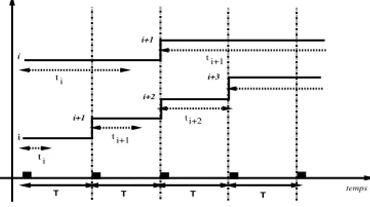
4.3. Distance between SPs
A receiver joins the next level at the receipt of a synchronization point provided that the time spent on a level is at least given by Equation 6. Therefore, these packets (SP) should not to be too much spaced because the convergence time can be too long. And worse, if the traffic is in competition with TCP, fairness can be lost. Therefore, the distance has to be short. However, we will see in section 4.4 that too short a distance has some shortcoming too. So we need to find a trade-off. As RLC does, we can give to this distance a fixed value whatever the session is, and the receiver on arrival of a synchronization point will subscribe to the next level if it has spent on the actual level, , more than units. This can lead, in the case of very shorts RTTs (and only in this case), two different concurrent sessions1to operate on the same
cycle length. Indeed, if the RTT is too short then and subscriptions will be
t t i i+1 i+1 T T T T i t i i+1 i+2 i+3 t i+1 i+2 t temps i
Figure 4. The difference between and
H T D P && T D T D S A P P && SP && ti > T P && SP SP && ti < T D P
P: loss ratio > threshold P: loss ratio < threshold SP: arrival of SP SP: normal packet
Figure 5. Protocol state machine
made after . Like RLC, this would lead to fairness in number of levels, instead of fairness in throughput. Therefore we have chosen proportional to the base layer data rate. Let this interval be:
Figure 4 shows the difference between the length of and in two examples, the lower one corresponds to shorter than and the upper one to the opposite.
The RLC synchronization points are designed to be exponentially spaced, ie the higher the level, the larger the distance between the SPs. In the case of our protocol, the distance between SPs is the same for every level. Thus, in case of short RTTs the receiver can go up quickly in the levels, and in the opposite case, its increase rate will be limited by the length of .
4.4. The RLS state machine
The proposed protocol, RLS (for “Receiver-driven Layered multicast with Syn-chronization points”), can be presented in the form of a state machine with 4 states
(see figure 5): the steady-state (S), add state (A), hysteresis state (H) and drop state (D).
On arrival of a synchronization point in state (S), the receiver has to compute the time spent at the actual level . If this time is greater than , as defined in Formula 6, it joins the next level (A), otherwise it stays at the actual one and goes into a deaf period (H). This deaf period is necessary to avoid misinterpretations. Indeed, without the presence of this period, the following scenario can happen:
Let and be two receivers behind a bottleneck (topology 2(a)), respectively members2 of level and , with, and the maximum level tolerated by the
shared path. Assuming that on arrival of a SP the receiver has spent at least
3 at its level which is not the case of . The latter feeling congestion will react by
dropping layer . This destruction is useless because layer will continue to transit the bottleneck. This can become annoying if the RTT from the source to is much longer than to . Imagine that and , without the deaf period will continue to drop its layers as being illustrated in Figure 6. On the left, we show the successive drops in levels leading to the decrease in throughput as shown right.
0 200000 400000 600000 800000 1e+06 1.2e+06 1.4e+06 0 20 40 60 80 100 120 140 160 180 200 throughput in bps Time in seconds R2 R1 1 2 3 4 5 6 7 8 0 20 40 60 80 100 120 140 160 180 200 Levels Time in seconds R1 R2
Figure 6. Necessity of a deaf period
If the receiver feels loss out of the deaf period, it computes the loss ratio over 1 RTT. If it is greater than the threshold defined in Equation 2 the highest layer is dropped (D).
To avoid reacting to a join attempt by leaving multiple subscription levels, the receiver does not react to losses for some time after dropping a layer. The purpose of this delay is to take into account the time necessary for the nearest router to react to the leave request. One can think that in the case of severe congestion, receiver should destroy several layers instead of one. But, we think that with the quantity of TCP traffic in networks, congested link is likely to be shared by several TCP traffics that will simultaneously decrease their data rate. This will release the path so that more than one drop would be useless.
To compute the round-trip-time, we had thought to do a ping at the beginning of the session from the receiver to the source and use it during all the session (as [AïT 99a]). This idea was fast abandoned because the results would strongly depend on the ping
. The notion of “member of level ” means “the maximum subscription level is ”. . = where is receiver ’s round-trip-time.
instant. We have opted for making a ping at the A-S and D-S transitions, and make exponential smoothing. Thus, RTT is computed as:
with
5. Simulations
We’ve identified two parameters and ’ in the previous section. We have tuned them to carry out our simulations. Each receiver stays at its level during:
where is an integer number of intervals or equivalently:
which means that it remains at its level during:
if
The tuning of the parameters depends on whether we want to privilege short RTTs or long ones. To find a good compromise, we have done several simulations with different values of the parameters and have found that setting the parameters to 1 ( ) gives good results in all cases.
For our simulations we use the network simulator NS ([MCC ns]) and the previous values for and . We use also data rates exponentially spaced between a level and the subsequent one by a factor of 2, i.e. . We will start by showing that intra-session fairness is provided, then we will show that the inter-sessions fairness is provided towards TCP and towards other RLS sessions.
5.1. Several receivers
In this section, we will just show the interest of deaf periods, that of synchroniza-tion points being already known. We repeat experiments done in secsynchroniza-tion 4.4 but with a deaf period. Figure 7 shows that receiver comes after receiver , goes up quickly and congests the link, but the receiver does not react to the congestion caused by the failed attempts and continue to climb the levels.
5.2. RLS versus TCP
5.2.1. Reminder
At first we want to remind what previous studies ([LEG 00] and [ELK 00]) had qualified as extreme cases i.e. which gives the worst results:
1 2 3 4 5 6 7 8 0 20 40 60 80 100 120 140 160 180 200 Levels Time in seconds R1 R2
(a) The growth in term of levels
0 200000 400000 600000 800000 1e+06 1.2e+06 1.4e+06 0 20 40 60 80 100 120 140 160 180 200 Throughput in bps Time in seconds R2 R1
(b) The growth in term of data rate
Figure 7. 2 different RLS receivers beginning at different moments
– TCP begins before the multicast protocol when the RTT is short. – TCP begins after the multicast protocol fort long RTTs.
In the first case, TCP is so aggressive that it prevents the multicast protocol (RLM, RLC) to get a reasonable share of the capacity. In the second case, TCP is so slow and so vulnerable that it cannot get a reasonable throughput. This happens because TCP works over a cycle proportional to the RTT which is not the case for the other multicast protocol. We will see that RLS performs much better in the extreme cases.
5.2.2. Simulations
We use the topology of Figure 2(b) with one TCP source and one RLS receiver to test the behaviour of both traffics. The parameters values are: Kbps and packet size = 1000 bytes. We will illustrate only the extreme cases.
Figure 8(a) shows the sharing in the first extreme case, i.e. short RTT when TCP begins before RLS. We see that the TCP traffic decreases to allow RLS to acquire some bandwidth. The sharing ratio, , is about 3, which is a reasonably good ratio4.
And figure 8(b) illustrates the second extreme case, with long RTTs, and TCP begins after RLS. The latter drops its highest layer to allow TCP to get more bandwidth. The share ratio is about 1/3. In conclusion:
where is equal to 3 which is a good k-bounded fairness.
. ratio = 3 means that if the perfect sharing would give layers, here the receiver gets layers. Indeed, suppose that the bandwidth of the bottleneck is . The perfect share is
. If a receiver gets layers instead of , it will get . Thus TCP gets and the ratio becomes 3.
0 100000 200000 300000 400000 500000 600000 0 20 40 60 80 100 120 140 160 180 200 Throughput en bps Time in seconds RLS TCP (a) Short RTT 0 100000 200000 300000 400000 500000 600000 0 100 200 300 400 500 600 700 800 Throughput in bps Time in seconde "RLS" TCP (b) Long RTT
Figure 8. The share of bottleneck
To better illustrate the dependence of the sharing ratio according to the round-trip-time we carried out several experiments where we changed only the propagation delay. We have done it for RLM and RLC too (for more results concerning these two protocols, refer to [LEG 00]). The chosen cycle is 8 seconds and all sources begin simultaneously. The results are illustrated on Figure 9.
0 1 2 3 4 5 0 200 400 600 800 1000 1200 1400
ratio tcp / other traffic
propagation delay in milliseconds RLC RLM RLS
Figure 9. RLM, RLC and RLS according to the one way delay
The RLS curve does not approach zero for long RTTs, and does not diverge for short RTTs. The RLM and RLC curves do not have these properties.
REMARK. — By choosing the data rate of the base layer and the packet size in such a way that the ratio is small, we can clearly improve the results obtained in the case of short round-trip-times. Indeed, when the growth in the levels is slowed down by the cycle length .
5.3. Fairness towards another RLS session
RLC did not succeed in providing fairness towards another RLC session for the reasons evoked in section 3.6. We will show that RLS fulfills this requirement. We use two different sessions, one with equal to 8 Kbps and the other with equal to 32 Kbps. To put us in an unfavourable case, the session with the smallest base layer begins when the other one has reached its optimal level. Figure 10 illustrates the result. We see that both sessions get the same bandwidth at the left of the figure, which corresponds to different levels as shown at the right of the figure.
0 200000 400000 600000 800000 1e+06 1.2e+06 0 100 200 300 400 500 600 Throughput in bps Time in milliseconds session_1 session_2 1 2 3 4 5 6 7 0 100 200 300 400 500 600 Levels Time in milliseconds session_1 session_2
Figure 10. The fairness in the case of 2 different sessions RLS
6. Conclusion
In this paper we have proposed a congestion control protocol for layered multicast to ensure:
1. fairness towards TCP,
2. a good coordination between the receivers to avoid misinterpretation, 3. fairness between sessions in terms of throughput (instead of levels).
We have simulated our protocol in differents situations, and the obtained results show that intra- and inter-sessions fairness is fulfilled and some fairness towards TCP is also satisfied.
We however plan to improve the following points:
– To compute the RTT, receivers send frequent pings to the source, which for large sessions can flood the source. We think that using the packet stamps to compute the RTT is possible and can reduce the number of pings.
– We will try to improve fairness ratio to one independently of the base layer throughput and the packet size.
– The state machine can be improved to reduce the number of unfruitful join ex-periments by monitoring the queuing delay.
7. References
[AïT 99a] AÏT-HELLALO., KUTYL., YAMAMOTOL., LEDUCG., “Layered Multicast using TCP-Friendly Algorithm”, report , 1999, University of Liege, Belgium.
[AïT 99b] AÏT-HELLALO., YAMAMOTOL., LEDUCG., “Cycle-based TCP-Friendly Algo-rithm”, Proceedings of IEEE Globecom’99, Rio de Janeiro, December 1999, IEEE Press. [ELK 00] ELKHAYATI., “Comparaison d’algorithmes de contrôle de congestion pour la vidéo
multipoints en couches”, Master’s thesis, University of Liege, Belgium, June 2000. [IAN 99] IANNACCONEG., RIZZOL., “A Layered Video Transcoder for Videoconference
Applications”, report , July 1999, University of Pisa, Italy.
[LEG 00] LEGOUTA., BIERSACKW., “Pathological Behaviors for RLM and RLC”,
Pro-ceedings of NOSSDAV’2000, Chapel Hill, North Carolina, USA, June 2000.
[MAT 97] MATHIS M., SEMKEJ., MAHDAVI, OTT T., “The macroscopic behavior of the TCP congestion avoidance algorithm”, Computer Communication Review, vol. 27, num. 3, 1997.
[MCC 95] MCCANNES., JACOBSONV., VETTERLIM., “Receiver-driven layered multicast”,
Proceedings of ACM SIGCOMM’95, Palo Alto, California, 1995, p. 117-130.
[MCC ns] MCCANNES., FLOYDS., The LBNL Network Simulator., Lawrence Berkeley
Lab-oratory, Software on-line ( ).
[PAD 00] PADHYE J., FIROIUV., TOWSLEYD., J K., “Modeling TCP Reno Performance: A simple Model and its emprical validation”, Proceedings of ACM SIGCOMM’2000, August 2000.
[RIZ ] RIZZOL., VICISANO L., CROWCROFTJ., “The RLC multicast congestion control algorithm”, Submitted to IEEE Network - special issue on multicast.
[VIC 98] VICISANOL., CROWCROFTJ., RIZZOL., “TCP-like congestion control for layered multicast data transfer”, Proceedings of IEEE INFOCOM’98, San Francisco, CA, March 1998.