Real time TEC monitoring using triple frequency GNSS data : a three step approach

REAL TIME TEC MONITORING USING TRIPLE FREQUENCY GNSS DATA:

A THREE STEP APPROACH

J.Spits(1), R.Warnant(2)

(1)

Royal Meteorological Institute of Belgium Avenue Circulaire, 3

B-1180 Brussels Belgium

Email : Justine.Spits@oma.be

(2)

Royal Meteorological Institute of Belgium Avenue Circulaire, 3

B-1180 Brussels Belgium

Email : R.Warnant@oma.be

INTRODUCTION

Triple frequency Global Navigation Satellite Systems (GNSS) will be operational in the next few years. The availability of a third frequency allows to develop several innovative techniques. We can cite triple frequency multipath analysis [1] or furthermore triple frequency ambiguity resolution algorithms, like Three Carrier Ambiguity Resolution (TCAR) for Galileo or Cascading Integer Resolution (CIR) for GPS [2].

Our goal here is to develop an improved Total Electron Content (TEC) monitoring technique based on triple frequency GNSS measurements. In a first step, we have developed a triple frequency simulation software, which enables us in a second step to develop and test our TEC reconstruction technique on realistic Galileo and GPS measurements.

In this method, code measurements are only used in the preliminary step. As a consequence, due to the fact that it is not affected by code hardware delays, the precision of the reconstructed TEC would be improved in regards with the usual dual frequency technique [3].

As the ionospheric delay –which mostly depends on the TEC– remains the main limitation of GNSS precision and reliability, an improved modelling of the TEC will allow to increase the precision and reliability of several GNSS navigation and positioning techniques.

TRIPLE FREQUENCY SIMULATION SOFTWARE

As the third frequency is not yet available, we have developed a software which allows to simulate realistic GNSS measurements. The final objective is to develop and to validate the TEC monitoring technique. As our TEC reconstruction technique uses both code and phase triple frequency (GPS and Galileo) measurements, the simulation software has to provide us all those data types. However, the validation of the software can only be made by comparing simulated and real GPS double frequency data.

Table 1 shows GPS and Galileo civil frequencies that will be used in this paper. For more readability, the E5b channel will be named L2, and the E5a channel L5, so that both GPS and Galileo frequencies will be named L1, L2, and L5.

Table 1. GPS and Galileo civil frequencies (MHz) GPS (MHz) Galileo (MHz)

L1 1575.42 L1 1575.42

L2 1227.60 E5b 1207.14

Code and phase measurements

If the propagation of GNSS signals took place in vacuum and if there were no clock errors or other biases, the code (or pseudorange) measurements would equal the geometric distance between the satellite at transmission time and the receiver at reception time. But this is not the case, and the equation of the code observables can be built as follows (in meters): i k p

P

_,

( )

pk i k p k p i k i p p i i k p i p i p i k p

D

T

I

c

t

c

t

r

d

d

M

P

_,

=

+

+

_,

−

Δ

+

Δ

+

Δ

+

+

_,

+

_,

+

σ

_, (1) with the super- or subscripts respectively identifying the satellite, the receiver and the carrier frequency (k = L1, L2 or L5).

k

p

i

,

,

Let us explain the successive terms of (1):

i p

D

Geometric distance (vacuum distance) traveled by the signal between the satellite at transmission time and the receiver at reception time. It is not yet corrected by the Earth rotation effect (see below).

i p

T

Tropospheric delay. This delay is always positive and is caused by the traveling of the signal through the neutral atmosphere. As it is a non dispersive medium in regards with GNSS frequencies, this delay is independent of the carrier frequency.

i k p

I

_, Ionospheric delay. This delay is always positive (code delay) and is caused by the traveling of the signal through the ionized atmosphere. As it is a dispersive medium in regards with GNSS frequencies, this delay is dependent on the carrier frequency.

The ionospheric delay can be written as follows:

TEC

f

I

k i k p 16 2 ,

10

3

.

40

=

(2)

with

TEC

= Total Electron Content, i.e. the number of free electrons in the column of unit area on the receiver-to-satellite path. In (2) as in the rest of this paper, the TEC is given in TEC units or TECU (with 1 TECU = 1016 electrons/m²);

and

f

_k the carrier frequency (in Hz).

i

t

c

Δ

Satellite clock error. This is the difference between the nominal time (i.e. the satellite clock reading) and the true time (in GNSS time scale) at transmission time. The term c is the velocity of light in vacuum (c = 299 792 458 m.s-1).

p

t

c

Δ

Receiver clock error. This is the difference between the nominal time (i.e. the receiver clock reading) and the true time (in GNSS time scale) at reception time.

i p

r

Δ

Earth rotation effect. It takes into account the fact that the Earth rotates during the propagation of the GNSS signals, which implies a change of the satellite position with respect to the terrestrial frame.

i k

d

Satellite code hardware delay. This delay depends on the carrier frequency.

k p

d

_, Receiver code hardware delay. This delay also depends on the carrier frequency.

i k , p

M

Code multipath delay. This delay is periodic and is caused by signal reflections. Moreover, it depends on the satellite elevation.

k , p

σ

Code measurement noise. This accidental error is linked to the measurement resolution and also depends on the satellite elevation.

The equation of the phase observables

Φ

i_p,k can be built quite similarly:

(

)

(

)

(

)

i k p k p i k p k p i k i p k p k i k i k p i p i p k i k p,

=

f

c

D

+

T

−

I

,

−

f

Δ

t

+

f

Δ

t

+

f

c

Δ

r

+

+

,

+

m

,

+

s

,

−

N

,

Φ

δ

δ

(3)

This is expressed in cycles, which involves the introduction of the frequency . However, this expression differs from (1) by the following terms:

k

f

i k p

I

_, Ionospheric delay. As the ionosphere is a dispersive medium, the code and phase measurements do not travel at the same speed; the ionosphere causes a phase advance (contrary to the code delay), so that we can put a minus sign before the ionospheric term in (3).

i k

δ

Satellite phase hardware delay.

k p,

δ

Receiver phase hardware delay.

i k p

m

_, Phase multipath delay.

k p

s

_, Phase measurement noise.

i k p

N

_, Integer ambiguity. It is the unknown integer constant representing the initial number of cycles (i.e. at the first epoch of observation) between the satellite and the receiver.

Let us mention that the phase hardware delays, multipath delays and measurement noise are lower than the corresponding code ones. As a consequence, although they are ambiguous, phase measurements are considered to be much more precise than code measurements.

Development of the software

In this section we will explain briefly how we have achieved the simulation of code and phase measurements as described in (1) and (3).

Let us explain GPS’s case. First, we have used several parameters transmitted in the real GPS navigation data in order to compute:

− the satellite position; it is computed in the Earth Centered Earth Fixed (ECEF) system by introducing the Keplerian parameters transmitted in the algorithm described in [4]; as a consequence, if the receiver coordinates are considered to be known, we can compute the term

D

i_p;

− the ionospheric delay i k p

I

, based on Klobuchar model; it is computed by using the eight Klobuchar

coefficients transmitted ; − the satellite clock error i

t

c

Δ

; it is computed by using the four clock coefficients and the relativistic effects parameters transmitted, as described in [4] ;

− the satellite code hardware delay i k

d

; it is computed by using the Time Group Delays (or

T

GD) transmitted.

Then, we have computed by applying a simple tropospheric correction model. In fact, we consider that the Zenith Total Delays (or

i p

T

ZTD

) are constant (ex. 2.40 m) and we divide them by a simple mapping function (i.e. the cosine of the zenith angle of the satellite) in order to obtain , which are Slant Tropospheric Delays (i.e. on the

receiver-to-atellite path):

z

T

_pi s

z

ZTD

T

_pi

cos

=

(4)

Furthermore, we have used a software based on real data to compute the receiver clock error

c

Δ

t

_p .

To take the Earth rotation effect into account, the original satellite coordinates (at transmission time – in ECEF at transmission time) must be rotated around the Z-axis of the system by an angle

α

, so that we obtain the corrected satellite coordinates (at transmission time – in ECEF at reception time). The

α

angle is defined as the product of the propagation time by the Earth’s rotational velocity. The corrected satellite coordinates allow to compute a corrected distance

D

i_p,2(in meters):

i p i p i p

D

r

D

_,2

=

+

Δ

(5) Moreover, as the receiver code hardware delays are generally considered to be constant in time, we simulate them as constant values.

Finally, the code multipath delay is computed on the basis of a Gaussian time correlated noise modulated by several characteristics, mainly the amplitude, the environment and the elevation factors. Quite similarly, the code measurement noise is simulated as a Gaussian noise characterized by its zero-mean and its standard deviation.

i k , p

M

k , p

σ

As far as the phase observables are concerned, we introduce the integer ambiguity by computing an integer constant value at each period for each satellite. Besides, we do not introduce hardware delays (satellite/receiver), multipath delays and measurement noise in the phase measurements for the moment. In fact, we consider as first assumption that all those delays are negligible with respect to our TEC monitoring technique developed below. Nevertheless, at each step we will justify why we are allowed to neglect their influence.

i k p

N

_,

Let us now come to Galileo’s case. We will only mention what it is different from GPS’s case.

Firstly, as there is only one Galileo test satellite (GIOVE-A) in orbit for the moment, we are not able to use real transmitted navigation data in our simulation software. However, we already know how the constellation is going to be built. By using the parameters described in [5] in a software based on Keplerian laws, we have simulated 30 satellites equally distributed and spaced on three orbital planes. Their inclination equals 56° and the semi-major axis 29 600 km. Moreover, in a first time we consider that the TEC vertical values ( ) are constant, so that the ionospheric delay is computed as follows: V

TEC

IP V k i k p

z

TEC

f

I

cos

10

3

.

40

16 2 ,

=

(6) The mapping function used to convert the vertical values into slant values

TEC

is the cosine of the zenith angle of the satellite at the ionospheric point (see [6]).

V

TEC

IP

z

In addition, we are not able to simulate

c

Δ

t

i,

c

Δ

t

_pand like in GPS’s case. So, as all the combinations used in the following TEC monitoring technique are independent of those first two parameters, we do not include them in (1) and (3). Moreover, we simulate as constant values (as for ).

i k

d

i k

d

d

_p,k

Validation of the software

The ultimate goal of this validation is to prove that the simulation software provides GPS and Galileo measurements realistic enough to test the TEC monitoring technique. We have first validated the triple frequency software on a double frequency GPS basis. Furthermore, as they are developed on the same basis, we make the assumption that the triple frequency GPS and Galileo software are also valid.

We have made the comparison between real and simulated double frequency GPS data for different stations and different days. After analysis, we can conclude that the differences remaining between real and simulated data can be explained by the uncertainties existing in the modelling of the several parameters defined in (1) and (3).

In fact, we have simulated the data again by introducing several more precise parameters, i.e. satellite coordinates and satellite/receiver clock errors provided by the International GNSS Service (IGS) as well as ZTD and TEC values computed with real GPS data. By doing this, the differences between real and simulated data became negligible (smaller than 1 meter). In other words, this means that all the other parameters (which were not improved) were already realistically simulated.

As a consequence, we can assume that it is sufficient to use the original version of the simulation software (i.e. without improvement of the modelling), because all the combinations that will be used for the TEC monitoring technique are independent of the first three error terms improved, and because the fourth one (the TEC) is precisely the major unknown.

TRIPLE FREQUENCY TEC MONITORING TECHNIQUE

Our final objective is to develop a triple frequency TEC monitoring technique. According to the definition of the TEC, it is important to note that the monitoring technique requires the use of code and phase measurements coming from one station only, and not double differenced measurements like in RTK positioning techniques for example.

First, we outline the theoretical aspects of our three step TEC reconstruction technique, and we validate it based on the triple frequency simulation software. The technique is explained in details below, both in theory and in practice.

First step

The objective of the first step is to resolve the extra-widelane (EWL) ambiguities

N

₂₅ (in cycles):

i L p i L p

N

N

N

₂₅

=

_{, 5}

−

_{, 2} (7) These ambiguities are integer numbers and can be estimated by making the difference between the widelane

ombination of L2/L5 phase measurements and the narrowlane combination of L2/L5 code measurements (in cycles): c 25 25 5 , 5 2 , 2 5 2 5 2 5 , 2 ,

P

N

R

c

f

P

c

f

f

f

f

f

i L p L i L p L L L L L i L p i L p

⎟

=

+

Δ

⎠

⎞

⎜

⎝

⎛

₊

+

−

−

Φ

−

Φ

(8)

The left hand side of (8) is thus the extra-widelane-narrowlane (EWLNL) combination; its wavelength

λ

₂₅ is given by in meters): ( 5 2 25 L L

f

f

c

−

=

λ

(9)

and

λ

25equals 5.861 m for GPS and 9.768 m for Galileo.

In fact, by computing this EWLNL combination, we obtain the extra-widelane ambiguities plus a residual term . This term corresponds to the sum (in cycles) of the satellite and receiver code hardware delays, the code multipath delays and the code measurement noise for L2 and L5 frequencies, multiplied by a combination of those frequencies (10). It should include the corresponding phase delays too, but here we can consider there are negligible

ith respect to the code ones.

25

N

25

R

Δ

w

(

)

(

)

⎟

⎠

⎞

⎜

⎝

⎛

₊

₊

₊

₊

₊

₊

₊

+

−

−

=

Δ

i L p i L p L p i L L i L p i L p L p i L L L L L L

M

d

d

c

f

M

d

d

c

f

f

f

f

f

R

5 _{5 , 5 , 5 , 5} 2 , 2 , 2 , 2 2 5 2 5 2 25

σ

σ

(10)

As a consequence, we have to determine if it is possible to resolve the EWL ambiguities (i.e. to fix them at their correct integer values) despite the existence of a residual term. For that purpose, we have to estimate if the influence of the residual term will exceed half a cycle.

In a first step, we can make the assumption that the influence of satellite and receiver code hardware delays is constant in time; therefore we have only estimated the influence of code multipath and code noise on the resolution of the EWL ambiguities.

Fig.1 and Fig.2 show two representative cases (resp. for GPS and Galileo) of the error on (in cycles) caused by code multipath and code noise. Because of the properties of code multipath and noise (Gaussian noise – see above), this is very variable. Moreover, the error does not exceed half a cycle in both cases, but it is by far smaller for Galileo’s.

25

N

We will now explain how it is possible to explain such a difference between GPS and Galileo’s cases.

Firstly, the most important part of the difference can be explained by the fact that the EWLNL combination wavelength is larger for Galileo (GA) than for GPS (GP):

66

.

1

25 25

=

− − GP GA

λ

λ

(11)

This means that if the different residual terms had exactly the same importance (in meters), would be 1.66 times arger for GPS. To prove it, we can compute the following ratio from (10):

25

R

Δ

l

66

.

1

5 2 5 2 5 2 5 2 5 2 5 2

⎟

=

⎠

⎞

⎜

⎝

⎛

₊

+

−

⎟

⎠

⎞

⎜

⎝

⎛

₊

+

−

GA L L L L L L GP L L L L L L

c

f

c

f

f

f

f

f

c

f

c

f

f

f

f

f

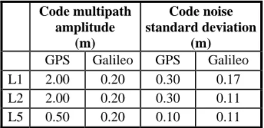
(12) In other words, how large is the wavelength, how small is the residual term, and how easier it is to resolve the ambiguities.

Secondly, the difference can be explained by the fact that the amplitude of code multipath and the standard deviation of code noise are lower for Galileo than for GPS. Table 2 presents the corresponding simulated values, which were chosen on the basis of observed values (for GPS L1 and L2) and of realistic predicted values (for GPS L5 and Galileo). As explained in [7], those values are lower for Galileo thanks to a new code modulation scheme and thanks to the fact that the power of Galileo signal will be double.

Fig.1. Influence of code multipath and code noise on

N

₂₅ for GPS (in cycles)

Table 2. Code multipath amplitude and code noise standard deviation (m) Code multipath amplitude (m) Code noise standard deviation (m) GPS Galileo GPS Galileo L1 2.00 0.20 0.30 0.17 L2 2.00 0.20 0.30 0.11 L5 0.50 0.20 0.10 0.11

In a second step, let us take the influence of satellite and receiver code hardware delays into account. In order to be able to resolve the EWL ambiguities, this influence should be lower than the remaining margin (i.e. the margin let by the influence of code multipath and noise in regards with half a cycle). The examples given in Fig.1 and Fig.2 show that it should be possible, especially for Galileo.

Let us give more details. We are able to estimate the influence of L1 and L2 GPS satellite code hardware delays on the basis of transmitted values. But we do not have any information about the amplitude of GPS receiver code hardware delays. In addition, we do not have many indications about the future Galileo code hardware delays. As a consequence, we would need real triple frequency GNSS data to do a more detailed analysis. For the moment anyway, we make the assumption that the sum of the three influences (code multipath delay, code measurement noise and code hardware delays) does not exceed half a cycle, so that it is possible to resolve the EWL ambiguities.

GD

T

Second step

The objective of the second step is to resolve the widelane (WL) ambiguities

N

₁₂ (in cycles):

i L p i L p

N

N

N

₁₂

=

_{, 2}

−

_{, 1} (13) These ambiguities are also integer numbers and could be estimated in a similar way to step 1, i.e. by making the difference between the widelane combination of L1/L2 phase measurements and the narrowlane combination of L1/L2

ode measurements (in cycles): c 12 12 2 , 2 1 , 1 2 1 2 1 2 , 1 ,

P

N

R

c

f

P

c

f

f

f

f

f

i L p L i L p L L L L L i L p i L p

⎟

=

+

Δ

⎠

⎞

⎜

⎝

⎛

₊

+

−

−

Φ

−

Φ

(14)

The left hand side of (14) is thus the widelane-narrowlane combination (WLNL); its wavelength

λ

₁₂ is given by (in eters): m 2 1 12 L L

f

f

c

−

=

λ

(15)

and equals 0.862 m for GPS and 0.814 m for Galileo. The residual term

Δ

R

₁₂ is similar to

Δ

R

₂₅in (10):

(

)

(

)

⎟

⎠

⎞

⎜

⎝

⎛

₊

₊

₊

₊

₊

₊

₊

+

−

−

=

Δ

i L p i L p L p i L L i L p i L p L p i L L L L L L

M

d

d

c

f

M

d

d

c

f

f

f

f

f

R

2 _{2 , 2 , 2 , 2} 1 , 1 , 1 , 1 1 2 1 2 1 12

σ

σ

(16)

Let us compare with the EWLNL’s case. Firstly,

λ

₁₂ is by far smaller than

λ

25 ; we obtain the following ratios, respectively for GPS and Galileo:

λ

25−GP

λ

12−GP

=

6

.

8

and

λ

25−GA

λ

12−GA

=

12

.

0

. Therefore, if the different

delays would have the same importance than in the L2/L5 case, the influence of

Δ

R

₁₂ would be respectively 6.8 and 12 times larger on the resolution of the ambiguities. Furthermore, the amplitude of code multipath as well as the standard deviation of code noise is slightly larger for the L1/L2 case than for the L2/L5 case (table 2). For those reasons, the

residual term automatically exceeds half a cycle, which makes the resolution of the WL ambiguities impossible by using the WLNL combination.

12

R

Δ

As a consequence, we have to form a combination that we will call differenced widelane (DWL) combination (in cycles):

(

) (

)

12 12 25 12 25 25 5 , 2 , 2 , 1 ,

−

Φ

−

Φ

−

Φ

+

=

+

Δ

−

Φ

i_pL i_pL i_pL i_pL

N

N

R

λ

λ

(17) This combination is based on the combinations of L1/L2 and L2/L5 phase measurements, i.e. and (respectively called WL and EWL combinations) as well as on the EWL ambiguities resolved at the first step. Let us note the that WL and EWL combination wavelengths correspond to the WLNL and EWLNL combination wavelengths i L p i L p, 1

−

Φ

, 2

Φ

i L p i L p, 2

−

Φ

, 5

Φ

N

₂₅ 12

λ

and

λ

₂₅ defined in (15) and (9).

The principles of this combination are the following. First, we have to subtract the EWL ambiguities from the EWL combination. Then, we have to multiply the result by the ratio between

λ

₂₅ and

λ

₁₂. As a consequence, by making the difference between the WL combination and this term, we obtain the WL ambiguities plus a residual term

.This residual term can be written as follows (in cycles):

12

N

25 12−

ΔR

i L p

I

b

R

_{12 25}

=

×

_{, 1}

Δ

₋ (18) with

b

a constant term depending on the three frequencies L1, L2, L5, which equals approximately 0.5 (m-1);

i L p

I

_{, 1} the ionospheric delay on L1 (m).

Because of , which can correspond to several cycles, it is impossible to fix the WL ambiguities at their correct integer values. Nevertheless, we obtain an approximation of which will be used in the third step.

25 12−

ΔR

12

N

Let us mention that (18) should include a term combining the phase hardware delays, the phase multipath delays and the phase measurement noise. Nevertheless, we can affirm that the importance of the ionospheric residual term in

ΔR

12−25 allows us to neglect the other residual terms, and allows us to resolve exclusively on ionospheric considerations (see below).

12

N

Third step

The objective of the third step is to use the results of the first two steps in order to achieve the monitoring of the TEC. or that purpose, we can form a system of two Geometric-Free (GF) phase combinations:

F

⎪⎩

⎪

⎨

⎧

+

−

=

Φ

−

Φ

+

−

=

Φ

−

Φ

i L p i L p i L p i L p i L p i L p i L p i L p

N

c

N

TEC

a

c

N

c

N

TEC

a

c

5 , 25 2 , 25 5 , 25 2 , 2 , 12 1 , 12 2 , 12 1 , (19) with

c

₁₂

=

f

_L1

f

_L2 ;

c

25

=

f

L2

f

L5 ;

a

₁₂

=

40

.

3

×

10

16

(

f

_L1

c

)

(

1

f

_L2₂

−

1

f

_L2₁

)

;

a

₂₅

=

40

.

3

×

10

16

(

f

_L2

c

)

(

1

f

_L2₅

−

1

f

_L2₂

)

The availability of triple frequency measurements only allows to form two (and not three) independent double frequency combinations; anyway TEC can be reconstructed directly based on GF phase combinations. Contrary to the usual dual frequency TEC monitoring technique which is described in [3], the precision of the reconstructed TEC will not be affected by code hardware delays. As a consequence, even if its precision would be affected by phase delays (hardware, multipath and noise), it should be significantly improved (one order of magnitude in regards with 2-3 TECU).

We can see in (19) that, by the use of those GF combinations, all the terms relative to the geometry, clocks... disappear, so that the TEC and the three integer ambiguities are the only remaining unknowns. As there are four unknowns, the system can not be resolved. However, the values of the resolved EWL ambiguities (first step) as well as the values of the approximated WL ambiguities (second step) can be introduced in the system, so that there remain only two unknowns. By replacing by (13) in the first equation and by (7) in the second, the system can be written as follows:

25

N

12

N

i L p

N

_{, 1}

N

i_p,L2

−

N

₁₂

N

i_p,L5

N

i_p,L2

+

N

₂₅

(

)

(

)

⎪⎩

⎪

⎨

⎧

−

+

=

−

Φ

−

Φ

−

+

=

−

Φ

−

Φ

1

1

25 2 , 25 25 25 5 , 25 2 , 12 2 , 12 12 2 , 12 1 ,

c

N

TEC

a

N

c

c

c

N

TEC

a

N

c

i L p i L p i L p i L p i L p i L p (20)

with

TEC

and

N

i_p,L2the two unknowns.

Let us express the unknowns in function of the observations in a matrix form:

⎟

⎟

⎠

⎞

⎜

⎜

⎝

⎛

−

Φ

−

Φ

−

Φ

−

Φ

⎟⎟

⎠

⎞

⎜⎜

⎝

⎛

−

−

=

⎟⎟

⎠

⎞

⎜⎜

⎝

⎛

− 25 25 5 , 25 2 , 12 2 , 12 1 , 1 25 25 12 12 2 ,

1

1

N

c

c

N

c

c

a

c

a

N

TEC

i L p i L p i L p i L p i L p (21) or (22)

⎟

⎟

⎠

⎞

⎜

⎜

⎝

⎛

−

Φ

−

Φ

−

Φ

−

Φ

⎟⎟

⎠

⎞

⎜⎜

⎝

⎛

=

⎟⎟

⎠

⎞

⎜⎜

⎝

⎛

25 25 5 , 25 2 , 12 2 , 12 1 , 22 21 12 11 2 ,

c

c

N

N

c

n

n

n

n

N

TEC

i L p i L p i L p i L p i L p

At this moment, we are able to resolve the system. But as the WL ambiguities are not fixed at their correct integer values, the

TEC

and resulting values are inaccurate. Nevertheless, on the basis of two properties, we are able to fix the WL ambiguities at their correct integer values, so that we obtain the accurate values of

TEC

and . The first property is that the WL ambiguties are integer numbers, which makes their resolution easier. The second property is that in (22) a change of 1 cycle in the WL ambiguties causes a change of approximately 12 TECU in the TEC values. In fact, the term (by which is multiplied to compute the TEC) equals 12.196 TECU/cycle for GPS and 11.327 TECU/cycle for Galileo.

12

N

i L p

N

_{, 2} i L p

N

_{, 2} 11

n

N

₁₂

Those two properties can be used as follows in order to obtain the accurate values of

TEC

:

− In a first step, we use the approximated values of

N

₁₂ obtained from (17) in (22) in order to compute the inaccurate values of the TEC:

TEC

₁. The accurate values of the TEC will be named

TEC

₂.

− In a second step, we use the usual dual frequency TEC monitoring technique in order to compute a rough estimation of the TEC values (i.e. of

TEC

₂) named

TEC

est. This technique is based on the GF

combinations of L1 and L2 code and phase measurements and provides TEC values with a precision of 2-3 TECU. The method is described in [3].

− In a third step, we compute the difference between

TEC

₁ and

TEC

_est :

Δ

TEC

=

TEC

₁

−

TEC

_est. − In a fourth step, we concurrently use the two properties explained here above. In fact, as

Δ

TEC

give us an

approximation of the real error made on the TEC values (i.e.

TEC

₁

−

TEC

₂), we can compute 11

/ n

in order to obtain an approximation of the error made on

N

₁₂. Regarding to the precision of

est

TEC

and considering the second property, we can consider that this approximation is sufficient to fix 12

N

at their correct integer values. In other words, we are able to resolve the WL ambiguities.

TEC

Δ

− In a fifth step, we introduce the new values of

N

₁₂ in (22) in order to compute the accurate values of the TEC, i.e.

TEC

₂.

CONCLUSIONS

In conclusions, the availability of a third frequency allows us to develop an improved TEC monitoring technique which presents two main advantages. On one hand, the technique requires the resolution of EWL and WL ambiguities, what is relatively efficient. On the other hand, the technique is based on the resolution of two GF phase combinations using one station data only, which allows to reconstruct absolute TEC values with the precision of phase measurements.

Let us finally give some perspectives for our work. The availability of real Galileo data from GIOVE-A satellite, and more particularly triple frequency code and phase measurements, will allow us to validate our TEC monitoring technique on the three-step level and to test the reliability of the several assumptions.

REFERENCES

[1] A. Simsky, “Three’s the Charm – Triple Frequency Combinations in Future GNSS,” Inside GNSS, pp. 38-41, July-August 2006.

[2] P.Teunissen, P.Joosten, C.Tiberius, “A comparison of TCAR, CIR and LAMBDA GNSS Ambiguity resolution,”

ION GPS 2002, Portland, United States, 24-27 September, 2002.

[3] R. Warnant, E. Pottiaux, “The increase of the ionospheric activity as measured by GPS,” Earth Planets Space, 58, 1055-1060, 2000.

[4] GPS JOINT PROGRAM OFFICE 2000, “Navstar GPS Segment / Navigation User Interface,” Interface Control

Document (ICD-GPS-200), 138 p, 2000.

[5] Galileo Project Office, “GIOVE-A Navigation – Signal-in-Space,” Interface Control Document, 46 p, 2007. [6] B. Hofmann-Wellenhof, H.Lichtenegger, J.Collins, “GPS: Theory and Practice”, Spinger-Verlag, 370 p, 1997. [7] A. Simsky, J.-M. Sleewaegen, W. De Wilde, F. Wilms, “Galileo Receiver Development at Septentrio,” ENC