Modelling waterfowl abundance and distribution to inform conservation planning in Canada

(1)

Modelling waterfowl abundance and distribution to

inform conservation planning in Canada

Thèse

Nicole Barker

Doctorat en sciences forestières

Philosophiæ Doctor (Ph.D.)

Québec, Canada

(2)

(3)

Résumé

La planification systématique de la conservation requiert la sélection de certains milieux sur la base d’information quantitative. Dans cette thèse, j’ai étudié la sauvagine nicheuse de la forêt boréale canadienne comme étude de cas. Les objectifs généraux étaient : 1) générer des informations sur l'abondance de la sauvagine utiles pour la planification de la conservation; 2) évaluer les effets de différentes méthodes de planification systématique sur la conservation de la sauvagine. Dans le chapitre 1, j’ai développé des modèles d'abondance d’espèces (MAE) à l’aide de modèles d’arbres de régressions répétées. Puisque l’évaluation statistique de ces modèles a démontré qu’ils performent bien, j’ai suggéré qu’ils soient utilisés pour planifier la conservation. Dans le chapitre 2, j’ai évalué les effets de l’agrégation des abondances de différentes espèces de sauvagine avant ou après la construction des MAE. Les résultats étaient similaires entre les deux stratégies de modélisation, ce qui suggère que la stratégie choisie n’aura que peu d'impact sur la planification de la conservation. Dans le chapitre 3, j’ai utilisé des cartes d'abondances d'espèces afin de réévaluer les hypothèses concernant les affinités de différentes espèces de sauvagine pour des biomes utilisés pour la nidification en Amérique du Nord. Onze espèces ont sélectionné les prairies-parcs à peuplier faux-tremble tandis que cinq espèces ont sélectionné la forêt boréale. Les espèces boréales n’étaient toutefois pas les plus abondantes dans le biome qu’elles ont sélectionné, ce qui met en évidence l'importance de tenir compte de la sélection d'habitats lors de la planification de la conservation. Dans le chapitre 4, j’ai comparé deux méthodes de construction de réseaux d'aires protégées dans la zone boréale en regard de leur capacité à prendre en compte la sauvagine et de la biodiversité globale. L'approche par filtre brut a construit des réseaux d’aires protégées plus représentatifs de la diversité écologique et tout en protégeant la sauvagine en proportion directe de la superficie du réseau. L'approche centrée sur la sauvagine pouvait protéger une plus grande proportion de la sauvagine, mais était plus pauvre écologiquement. Dans l’ensemble, ma thèse met en lumière les méthodes appropriées pour construire des réseaux de conservation à l’aide de MAE.

(4)

(5)

Abstract

In this thesis, I investigated the conservation of waterfowl in the Canadian boreal region as a case study. The overall goals of this thesis were to: 1) generate information on waterfowl abundance and distribution that can be used for conservation planning and other applications, and then; 2) evaluate how various modelling or conservation planning methods will influence conservation planning decisions. In Chapter 1, I created the foundational species abundance models (SAMs) upon which the remainder of the thesis was built. Boosted Regression Tree models performed well, statistically, and I suggested that they can be used for waterfowl conservation planning in Canada. In Chapter 2, I extended these SAMs to species groups and assessed the difference between aggregating waterfowl abundance before or after model-building. Results were similar between the modelling strategies, suggesting that the strategy chosen will have little impact on conservation planning decisions. In Chapter 3, I used species abundance maps to re-evaluate the assumptions regarding large-scale habitat selection by waterfowl within North America. Eleven species selected the prairie-parkland while five selected the boreal. Those selecting the boreal were not always the most abundant species in the region. In Chapter 4, I compared two methods of building protected area networks in the boreal biome, in terms of their performance for protecting waterfowl and overall biodiversity. The biodiversity-oriented approach built more ecologically representative networks while protecting waterfowl proportionately to network area. The waterfowl-oriented approach protected more waterfowl but poorly represented the biodiversity of the region. As a whole, my thesis sheds light on appropriate methods to follow when building and using species abundance models for conservation planning.

(6)

(7)

List of Tables

Table 1.1. Species and species groups included in this study, along with the feeding and

nesting guild assigned to each. ... 13

Table 1.2. Environmental variables used in Boosted Regression Trees of waterfowl abundance. ... 16

Table 1.3. Reclassification of Land Cover of Canada’s (2005) original 39 land cover classes to 16. ... 22

Table 1.4. Spatial autocorrelation results ... 40

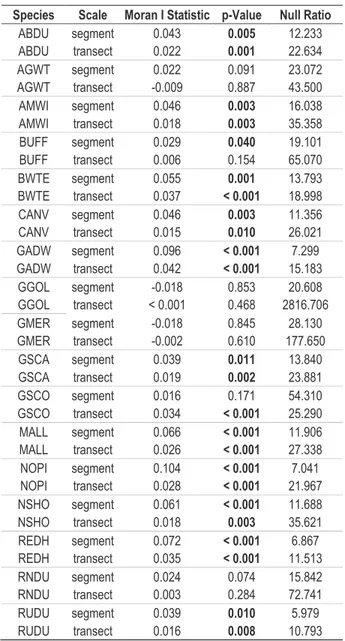
Table 2.1. Moran’s I statistic calculated at segment and transect scale. ... 95

Table 3.1. Metrics of biome selection. ... 113

Table 3.2. Summary of species' selection for (; positive selection) or against ( ; negative selection) biomes ... 121

Table 4.1. Parameter estimates and 95% confidence intervals (CIs) for multiple linear mixed-effects models of network effectiveness as a function of area target (10%, 20%, 35%, 50%), network type (BEACONs vs. WaHP), and study region (EBF vs. WBF) ... 181

Table 4.2. Parameter estimates and 95% confidence intervals (CIs) for linear regression model as a function of area target (10%, 20%, 35%, and 50), network (BEACONs vs. 21 different WaHP), and study region (EBF vs. WBF), plus their interaction ... 182

Table A1.1. Species and species groups included within the WBPHS database ... 198

Table A1.2 ... 204

Table A1.2. Major aims of papers, reports, and theses using WBPHS data or reviewing WBPHS methods ... 208

Table A1.3. Sampling coverage for each species for two time periods and the full time series ... 221

Table A1.4. Supplementary information that would benefit and expand the use of WBPHS data ... 230

(12)

(13)

List of Figures

Figure 1.1. Top: Survey strata and transects of the Waterfowl Breeding Population and Habitat Survey (WBPHS) in Canada. Bottom: Some major lakes, rivers, and

ecoregions referred to herein ... 14

Figure 1.2. Conceptual map summarizing the rationale behind our variable selection. ... 21

Figure 1.3. Evaluation metrics calculated from repeated sub-sample cross-validation ... 26

Figure 1.4. Mean prediction uncertainty across 17 species models. ... 28

Figure 1.5. Summed relative abundances (per km2_{) of all 17 species or species groups. .... 28}

Figure 1.6. The number of species with each variable class as the most influential variable ... 31

Figure 1.7. The cumulative relative influence of each class, for the full species set, and for each feeding/nesting guild. ... 31

Figure 2.1. Study area and protected areas. ... 81

Figure 2.2. Three modeling strategies to generate predictions of species group abundance from species-level data. ... 85

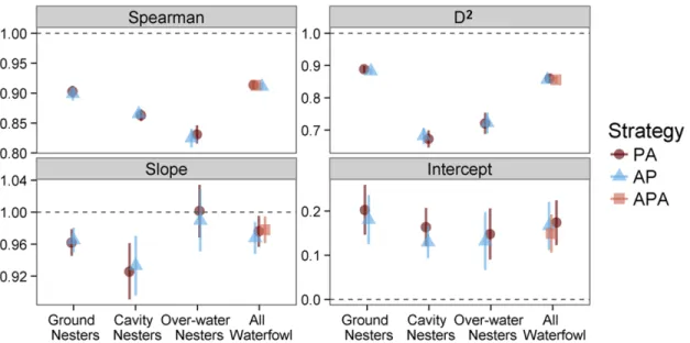
Figure 2.3. Evaluation statistics ... 87

Figure 2.4. Relative differences between guild-level waterfowl pair densities predicted by predict first, assemble later (PA) and assemble first, predict later (AP) modeling strategies ... 88

Figure 2.5. The mean ± SD proportion of each species group’s predicted population contained within existing Canadian protected areas ... 89

Figure 2.6. Maps of residuals from BRT models ... 96

Figure 2.7. For each waterfowl group, the variance of the estimated model calibration parameters was similar across the different modelling strategies. ... 97

Figure 2.8. Predicted density (pairs/km2_{) for three nesting guilds from predict first,} assemble later (PA) and assemble first, predict later (AP) modeling strategies ... 98

Figure 2.9. Predicted density (pairs/km2_{) for All Waterfowl ... 99}

Figure 2.10. Differences in predictions of All Waterfowl from the three modeling ... 100

Figure 3.1. Study area and biomes used in these analyses. ... 106

Figure 3.2. Conceptual model of the quantification of large-scale habitat selection ... 107

Figure 3.3. Example abundance and range data used in these analyses ... 111

Figure 3.4. Mean predicted population densities (pairs/km2_{) for 17 waterfowl species in} each of five biomes ... 115

(14)

Figure 3.5. The proportion of each species’ range and population contained within the a) prairie-parkland, boreal, and other biomes, or b) prairie, hemi-boreal, boreal, and other biomes ... 116 Figure 3.6. Two metrics of selection for prairie-parkland, prairie, hemi-boreal, and boreal

biomes ... 118 Figure 4.1. Western Boreal Forest (WBF; dark green) and Eastern Boreal Forest (EBF;

light green) study regions and area targets (in km2_{) for protected areas networks in}

each region. ... 158 Figure 4.2. One of 21 abundance maps used to build WaHP networks ... 162 Figure 4.3. Visual representation of the pairs of networks for which spatial overlap was

calculated. ... 163 Figure 4.4. Top five BEACONs networks of each of four area targets (columns) in the

western and eastern study regions ... 165 Figure 4.5. WaHP networks for four groups of species (rows) within each area target

(columns) in the western and eastern study regions. ... 166 Figure 4.6. Spatial overlap between the top 10 BEACONs and the 21 different WaHP

networks ... 167 Figure 4.7. Network effectiveness as a function of area target, network type, and region 168 Figure 4.8. Ecological representation as a function of area target, network (21 WaHP +

BEACONs), and study region ... 170 Figure 4.9. Beacons networks ranked 6th-10th of the top 10 ... 177 Figure 4.10. WaHP networks for individual waterfowl species (rows) within each area

target (columns) in the western and eastern study regions. ... 178 Figure 4.11. Proportion of each study region (Left: West; Right: East) captured within

networks that contain specified proportions of the waterfowl population ... 180 Figure A1.1. Sampling design (strata and fixed-wing transects) of the WBPHS ... 195 Figure A1.2. Sampling design in key years ... 197 Figure A1.3. Sampling design (fixed-wing transects and helicopter plots) of the Eastern

Survey... 201 Figure A1.4. Timeline of the Waterfowl Breeding Population and Habitat Survey ... 213 Figure A1.5. Apparent replication in survey effort from 1955-2011 ... 215 Figure A1.6. Numbers of segments present in the online population database each year . 215 Figure A1.7. Proportions of sampled segments within each species’ range for key years in

(15)

List of Supplements

Supplement 1.2. Individual species results ... 41

Supplement 2.2. Assessment of bias-variance tradeoff ... 97

Supplement 2.3. Predicted density (pairs/km2_{) for waterfowl groups ... 98}

Supplement 2.4. Differences in predicted density of All Waterfowl ... 100

Supplement 3.1. Biome descriptions ... 131

Supplement 3.2. Range delineation ... 134

Supplement 3.3. Selection metrics considered ... 142

Supplement 3.4. Results of Disproportionate Use metric ... 147

Supplement 4.1. BEACONs networks ... 177

Supplement 4.2. Individual species networks ... 178

Supplement 4.3. Waterfowl networks built for population targets ... 180

Supplement 4.4. Network effectiveness model results ... 181

Supplement 4.5. Ecological representation model results ... 182

Supplement A1.1. Glossary of terms ... 232

(16)

(17)

Acknowledgments

I have many people to thank for helping me achieve my dream of conducting applied conservation research.

I thank Steve Cumming for his supervision. For accepting the many revisions to my project direction. For his patience in filling the sometimes surprising gaps in my knowledge. For his streamlining of my sometimes wordy prose. I thank Marcel Darveau for his supervision. For his encouragement, kind words, and support. For speaking English with me. For helping me navigate subtler aspects of research and collaboration. For his unswaying confidence in my abilities. I thank Stuart Slattery for on-going discussions about the direction and application of my project. Our conversations were always useful, thought-provoking, and motivating. I still have a massive list of research questions I'd like to answer!

I thank the various members of my committees. Andy Royle provided discussion and practical assistance on some of the unrealized thesis chapters; I benefitted greatly from my visit to Patuxent and the hierarchical modelling workshop. Tom Nudds, with his wealth of waterfowl knowledge, asked important and challenging questions, encouraging me to questions my own assumptions. Eliot McIntire provided useful statistical and theoretical knowledge, as well as encouragement when I needed it. I thank Frédéric Raulier and Bob Clark for agreeing to serve on my evaluation committee, and for their several thought-provoking questions and suggestions.

Special thanks to Eliot McIntire, Josh Nowak, Chris Roy, Sebastien Renard, Etienne Racine, Mélina Houle, Sarah Bauduin, and Jerod Merkle for innumerable things, only a few of which are named here. To Eliot, Josh, and Chris: thank you for for including me in two self-directed statistics courses. I still think fondly about our time in the basement of ABP, teaching each other about Bayesian statistics, data simulation, and so much more. To Chris, Josh, and Etienne: thank you for teaching me about R; from the basics to spatial processing and ggplot2. To Etienne, Chris, Josh, and Seb: thank you for indulging me with the writing group; we had a good go of it for a year! To Mélina: thank you for your patience and assistance with all spatial processing issues, tasks, and questions. I enjoyed your cheerful and friendly

(18)

presence in the office. To Josh, Chris, Seb, Jerod, and Sarah for our weekly discussions at the "CKM"; it's always nice to broaden my sphere of knowledge beyond my own work. To Chris, Sarah, Sarah-Claude, Audrey, Laurie, and Marcel: I greatly appreciate your time and efforts in translating and revising my abstracts!

I thank all past and present members of the Metalab, PleinR, and DUC-QC that I haven`t mentioned otherwise. Those named here and those unintentionally forgotten: Sarah Bauduin, Nadia Bokenge Aridja, Aude Corbani, André Desrochers, Stéphanie Ewen, François Fabianek, Julie Faure-Lacroix, Hermann Frouin, Marie-Hélène Hachey, Toshinori Kawaguchi, Mélanie-Louise Le Blanc, Céline Macabiau, Jean Marchal, Yosune Miquelajauregui, Pierre Racine, Renée Roy, Lukas Seehausen, Maïa Sefraoui, Stéphane Bergeron, Laurie Bisson Gauthier, Stéphanie Boudreau, Rahim Chabot, Jérome Cimon-Morin, Audrey Comtois, Geneviève Courchesne, and Simon Perreault. I acknowledge my office mates for understanding my desire to rearrange the furniture configuration every few months. And for taking care of my plants in my absence. I thank the staff and students at the DUC-Quebec office, particularly Marcel and Bernard, for their kindness and understanding of my rudimentary French. I thank Dave Howerter, Mark Gloutney, Erling Armson, and those at the IWWR and Eastern Region of DUC for making me feel like one of the team.

The BAM team, especially Diana Stralberg and Peter Solymos, provided thought-provoking and useful discussion throughout my thesis. I thank Trish Fontaine and the BAM Steering Committee for including me in team activities; it was always inspiring and motivating. I also thank the BEACONs team for their discussion and support. Kim Lisgo provided a very useful tutorial on the use of Builder, and Pierre Vernier supplied code and assistance for use of Ranker code. Fiona Schmiegelow provided important discussion regarding the BEACONs philosophy and application.

I greatly appreciate the efforts of the USFWS and CWS in collecting, maintaining, and quality-checking the WBPHS data. I recognize substantial assistance from USFWS employees, including Emily Silverman, Kathy Fleming, Guthrie Zimmerman, Mark Otto, and Ken Richkus, Scott Boomer, and Mark Koneff, for answering questions and discussing the survey with me. I thank Dan McKenney and Pia Papadopol of Natural Resources Canada

(19)

for supplying the climatic data I used in this thesis. The efforts and time of Mélina Houle and Pierre Racine must be recognized for their PostGIS work. I thank NSERC, FQRNT, DUC, the IWWR, BAM, CEF, CSBQ, and the Fondation F.-K.-Morrow for financial support. I thank Steve, Marcel, Eliot, Céline Boivenue, Josh, Ann Nowak, Chris, Seb, Ariane Béchard, Melina, and Mélanie-Louise Léblanc for making me feel welcome in Quebec.

I thank my family. I thank my parents and in-laws for their support and help with my move to (and back from!) Québec. A special thanks to my mom for her time in my final year; I would not be near finished this thesis at this time if it weren't for her support. I thank my husband Kyle, for his continual support, both emotional and practical. For listening to me ramble about waterfowl, statistics, and conservation planning, even if he didn't always care or understand what I was talking about. For letting me talk through my problems aloud, and giving feedback on presentation of results. I thank my daughter Lily for keeping me laughing, and for taking such structured and predictable naps during which I ran analysis and wrote chapters.

(20)

(21)

Preface

This thesis consists of four data chapters and an Annex. I am the main author of each chapter, and all were written in English in a format suitable for submission to scientific journals. I completed much of the work for each chapter, including establishing research objectives, generating hypotheses, performing statistical analyses, interpreting results, generating figures, and writing. Colleagues helped with many of the above steps, as detailed below and in the Acknowledgments.

The first chapter summarizes the creation of species abundance models using long-term survey data of waterfowl. This article was written in collaboration with Steven Cumming and Marcel Darveau. It was published in 2014 in the journal Avian Ecology and Conservation with the title "Models to predict the distribution and abundance of breeding ducks in Canada". S. Cumming assisted with statistical details and suggestions for presenting results. M. Darveau provided assistance and discussion regarding waterfowl biology and interpretation of results.

The second chapter contrasts two strategies for building species abundance models of species groups (in this case, nesting guilds). The article was written in collaboration with Stuart Slattery, Marcel Darveau, and Steven Cumming. It was published in 2014 in the journal Ecosphere with the title "Modeling distribution and abundance of multiple species: Different pooling strategies produce similar results". S. Slattery helped motivate the research question and assisted with writing, M. Darveau guided presentation of results, and S. Cumming helped with statistics and by editing the writing.

The third chapter reinvestigates assumptions regarding selection for biomes in Canada by waterfowl species. In its current form, this chapter was written in collaboration with Mark Bidwell, Christian Roy, and Steven Cumming. M. Bidwell helped motivate the question and generate research hypotheses. C. Roy helped with research hypotheses and with interpretation and presentation of results. S. Cumming provided insight on statistical analysis, and revised the writing. While not listed as authors, Marcel Darveau, Tom Nudds, and Bob Clark provided additional comments on the framing and discussion of the chapter. This

(22)

chapter is being prepared for submission to a scientific journal; the specific journal has yet to be determined.

The fourth chapter compares two methods of creating protected areas networks in boreal Canada. In its current form, this chapter was written in collaboration with Steven Cumming and Marcel Darveau. M. Darveau provided insight into research context. S. Cumming helped motivate the research questions and revised the writing. Other colleagues not listed provided support for use of the BEACONs method, and their contribution is noted in the acknowledgements. This chapter is being prepared for submission to a scientific journal; the specific journal has yet to be determined.

The Thesis Annex reviews the Waterfowl Breeding Population and Habitat Survey from the perspective of a secondary user. In its current form, this appendix was written in collaboration with Eric Reed and Steven Cumming. E. Reed added portions of writing, notably to the sections on the Eastern Survey. S. Cumming revised the writing. This chapter is being prepared for submission to a scientific journal; the specific journal has yet to be determined. The paper has not been fact-checked or approved by the USFWS.

(23)

General Introduction

Wildlife Conservation and Management

Wildlife conservation and management aims to preserve biodiversity and species' populations against the negative impacts of human activities (Organ et al. 2012). For game species, this means preserving populations at levels that permit sustainable use (Festa-Bianchet and Apollonio 2003). In the initial stages of the European settlement of North America, little management or conservation of animal species occurred (Anderson and Henny 1972). This resulted in extinctions of several species, including the passenger pigeon (Ectopistes migratorius), Steller’s sea cow (Hydrodamalis gigas), great auk (Pinguinus

impennis), ivory-billed woodpecker (Campephilus principalis), and Labrador duck

(Camptorhynchus labradorius; Bolen and Robinson 2003 pp. 12–13). Other species, including the wood duck (Aix sponsa), wild turkey (Meleagris gallopavo), and bison (Bison

bison), suffered drastic population declines before humans began actively managing

populations for future use (Bolen and Robinson 2003 p. 14).

When wildlife management gained popularity c. 1900, the focus was on managing survival rates (Leopold 1987 p. xvii), primarily by limiting hunting (Leopold 1987 p. 13, Bolen and Robinson 2003 p. 3). That the wood duck population initially rose following the implementation of this technique in the early 1900s showed the potential of managing populations by reducing hunting mortality. However, the subsequent stagnation of the wood duck population at levels below those desired revealed the need for another component of management (Bolen and Robinson 2003 p. 25), specifically, the protection, enhancement, or restoration of habitat to increase carrying capacities and ultimately the population size and sustainable yield of species (Leopold 1987 pp. 5, 47, Osnas et al. 2014). This habitat-focused approach was not widely implemented in the early days of game management (Bolen and Robinson 2003 p. 20). It was first formalized in 1936 with a migratory bird treaty with Mexico calling for refuge regions (Leopold 1987 p. xx). Increases in wood duck populations after implementing widespread use of nesting boxes in the 1940s demonstrated that wildlife management via habitat modification can complement management by harvest regulations (Bolen and Robinson 2003 p. 25).

(24)

In protecting or restoring habitat, we assume that providing land and food resources will raise carrying capacity, and therefore increase population size (Leopold 1987, Bolen and Robinson 2003, Osnas et al. 2014). However, early game managers had a better understanding of species’ anatomy and taxonomy than of their behaviour, vital rates, population sizes, or ecological requirements, as highlighted by Aldo Leopold:

The early attempts to apply biology to the management of game as a wild crop soon disclosed the fact that science had accumulated more knowledge of how to distinguish one species from another than of the habits, requirements, and inter-relationships of living populations. Until [the 1930’s] science could tell us, so to speak, more about the length of a duck’s bill than about its food, or the status of the waterfowl resource, or the factors determining its productivity.

(Leopold 1987 p. 20)

Leopold initiated the movement towards incorporating science, specifically ecological knowledge, to improve effectiveness of wildlife management (Bolen and Robinson 2003 p. 466). In particular, he promoted measurement of various characteristics of game populations, including population size, sex and age ratios, productivity, mortality, and community composition (Leopold 1987 p. 140).

Waterfowl Conservation and Management: Importance of Population Monitoring

Throughout the 19th_{century, overharvest directly reduced waterfowl populations while}

human activities such as logging and agriculture decreased the habitat available for breeding waterfowl (Anderson and Henny 1972, U.S. Fish and Wildlife Service 2004). Harvest limits were imposed in some U.S. states during the 1870s, but they were poorly enforced. It was recognized in the early 20th_{century that more effort was necessary to protect continental}

waterfowl populations (U.S. Fish and Wildlife Service 2004). Various treaties and legislation, including the U.S. Migratory Bird Treaty Act and the Canadian Migratory Birds Convention Act, mandated national responsibility to manage waterfowl harvest at sustainable levels (U.S. Fish and Wildlife Service 2004). As part of the latter act, money was allocated to create wildlife refuges to protect waterfowl populations (Anderson and Henny 1972). However, populations continued to decline due to a multi-decade drought in the prairies (Anderson and Henny 1972). Additional legislation in the late 1930s redirected sales taxes on ammunition and sporting arms towards waterfowl programs. In 1938 Ducks Unlimited

(25)

Canada was established to aid in habitat acquisition and improvement in Canada (Anderson and Henny 1972).

It was soon recognized that ecological knowledge was necessary to successfully manage continental waterfowl populations, regardless of whether top-down (harvest-based) or bottom-up (habitat-based) techniques were used (Osnas et al. 2014). Various programs were established over the first half of the 20th_{century to estimate population sizes on species’}

breeding and wintering grounds and to quantify the distributions of waterfowl across North American (Anderson and Henny 1972, U.S. Fish and Wildlife Service 2004). Waterfowl banding programs were initiated in 1922 and then refined in the 1940s and 1950s; these were and still are used to delineate migratory routes and to estimate population sizes and survival rates (Anderson and Henny 1972). A wintering ground survey was initiated in 1934 to estimate population sizes; information from this survey was used to guide harvest regulations for many years (Anderson and Henny 1972). A survey to estimate harvest rates was initiated in 1952, and the Parts Collection Survey was initiated in 1960 to obtain information about annual production via age and sex ratios (Anderson and Henny 1972). Experimental aerial surveys of breeding waterfowl populations began in 1947 when aircraft and pilots became available after World War II (Anderson and Henny 1972). Techniques were refined throughout the early 1950s until the first coordinated survey of the North American waterfowl breeding grounds, the Waterfowl Breeding Population and Habitat Survey, became operational in 1955 (Smith 1995, U.S. Fish and Wildlife Service 2004). This survey, and the other efforts described above, make up the North American waterfowl monitoring program. This program developed over many decades to become what is now “believed to be the most extensive, comprehensive, long-term annual wildlife survey effort anywhere” (U.S. Fish and Wildlife Service 2004).

Secondary Uses of Waterfowl Survey Data

In an Annex to this thesis, I describe and review the Waterfowl Breeding Population and Habitat Survey (Smith 1995), the major aerial survey used to monitor continental waterfowl populations. The primary use of this survey is to estimate species’ annual breeding population sizes at the continental level. My review is written from the perspective of a secondary user

(26)

– a researcher who seeks to apply the dataset to research questions that it was not designed to address. I begin by summarizing the survey protocol and the database structure. I then provide some examples of secondary uses and describe how types of secondary uses changed over time. The bulk of the material addresses features of the survey and of the resultant database that should be accounted for by secondary users. My hope is that the review and recommendations contained therein will promote further secondary applications of the survey data to problems in ecology, biogeography, and wildlife conservation.

Species Abundance Models

Species distribution models (SDMs) are correlative and predictive models that relate geographical patterns in species’ occurrence or abundance data to environmental information (Guisan and Zimmermann 2000, Elith and Leathwick 2009b). SDMs have been variously called habitat models, bioclimatic models, ecological niche models, and resource selection functions, among other things, though some of these terms reflect slight methodological variations (Elith and Leathwick 2009b). Within this thesis, I draw a distinction between occurrence-based SDMs, which use presence-absence or presence data, and abundance-based SDMs, which use count data. I refer to the latter as Species Abundance Models, or SAMs, and they are the focus of my thesis.

The general technique is the same for SDMs and SAMs. Observations of species’ presence or abundance from a sample of locations are related to the environmental conditions at those locations via some statistical model (Guisan and Zimmermann 2000). Typically the environmental conditions are derived from remotely sensed landscape data or spatially interpolated climate data. A variety of statistical techniques can be used, including linear regression, ordination and classification methods, and Bayesian models. The resulting model can then be used to generate predictions for unsampled locations based on the environmental conditions at those locations (Elith and Leathwick 2009b). An SDM or SAM is a quantification of the conditions where the species occurs most often or in highest abundance, which can then be extrapolated to predict the potential distribution or abundance of a species in geographic space (Kearney and Porter 2009), based on the distribution or abundance in environmental space (Elith and Leathwick 2009b). The creation and prediction of SDMs and

(27)

SAMs can therefore be considered an application of the Hutchinsonian niche concept (Kearney and Porter 2009).

SDMs and SAMs achieve two main aims: 1) they improve the current understanding of species’ ecology, including habitat associations, range limits, and geographical patterns in abundance; and 2) they generate maps of species’ occurrence or abundance which can be used in further applications (Elith and Leathwick 2009b). These models and the resulting maps have been, among others, applied to investigations of ecology and evolution (Peterson et al. 1999), biogeography and range (Anderson et al. 2002a, Hugall et al. 2002), invasive species (Buchan and Padilla 2000, Elith et al. 2010), the spread of disease (Venier et al. 1998), biological indicators and surrogates (Ferrier and Watson 1997, Utzinger et al. 1998, Bonn and Schröder 2001), climate change impacts (Araújo et al. 2004a, Thuiller 2004, Araújo and Luoto 2007), and conservation planning (Schadt et al. 2002, Meggs et al. 2004).

SAMs of Waterfowl Species

Chapter 1 of this thesis focuses on the creation and evaluation of SAMs of waterfowl species using data from the Waterfowl Breeding Population and Habitat Survey. In this chapter, I describe the statistical models, evaluate their predictive performance, summarize some overall patterns gleaned from these models, and review some of the potential limitations and areas for future research. In a supplement to this chapter, I present the maps of predicted abundance and compare them to published range maps. I also showcase the most important predictor variables for each species, and discuss the potential biological relevance of these variables. The primary goal of this chapter is to create predictive abundance maps of waterfowl species for subsequent analysis.

SAMs of Waterfowl Species Groups: Aggregate Species Before or After Modelling?

Chapter 2 of this thesis extends the SAMs from the previous chapter to generate models of species groups. When building SAMs for groups of species, one can either create individual models for each species and then sum the predictions (predict first, assemble later), or one can aggregate the observations and create one model for the resultant sum (assemble first,

predict later; Ferrier and Guisan 2006). In this chapter, I build models for Cavity Nesters,

(28)

I then compare the predictive ability of the resultant models and I compare the resultant patterns in predicted abundances. To assess implications of different modelling strategies for conservation planning, I quantify the proportion of the predicted population contained within existing Canadian protected areas. The primary goal of this chapter is to provide some insight into which strategy is most appropriate for conservation planning in Canada.

Waterfowl Conservation

The North American Waterfowl Management Plan (NAWMP) aims to achieve and maintain waterfowl populations at levels that allow sustainable hunting and other uses (NAWMP Committee 2012). Integral to this goal is the preservation and establishment of sufficient waterfowl habitat to maintain populations at desired levels (NAWMP Committee 2012). Emphasis is placed on "permanent protection of naturally-functioning systems" to ensure long-term sustainability of habitats (NAWMP Committee 2012).

Ducks Unlimited Canada, Ducks Unlimited Inc., and Ducks Unlimited de Mexico (collectively, DU) are nonprofit conservation organizations that work to preserve, enhance, or restore waterfowl habitat to help achieve NAWMP objectives. One region that has received increasing interest in recent years is the Canadian boreal forest (Ducks Unlimited Canada 2010). Many North American waterfowl breed in the western boreal forest (Slattery et al. 2011), so conservation in this region is essential for maintaining or increasing waterfowl populations (NAWMP Committee 2012).

Importance of the Boreal Region to Waterfowl

Chapter 3 focuses on waterfowl biogeography. In this chapter, I use maps of predicted abundance from Chapter 1 to evaluate assumptions regarding waterfowl distributions within North America. I calculate metrics of selection based on proportions of species’ ranges and abundances’ within some biomes meaningful for waterfowl management: the prairie-parkland, boreal, prairies, and hemi-boreal, where the prairie-parkland is comprised of the western hemi-boreal and the prairies. I compare these metrics to a null assumption of no selection using a randomization test to determine the strength of selection for each biome. The primary goal of this chapter is to assess the importance of and selection for various

(29)

biomes in North America. A second goal is to create an index of “borealicity” for North American waterfowl.

Conservation Planning Objectives: Target Species vs Biodiversity

Many boreal breeding waterfowl species are thought to occur at low densities over large areas (Slattery et al. 2011), presenting a challenge for the design of protected areas (Wells 2011b). Systematic conservation planning involves identifying which land to allocate to reserves and which to allow for development, based on explicit goals (Margules and Pressey 2000). One goal of a protected area may be to preserve exploited species to sustain future harvest; this tactic has a long history in environmentalism and conservation (Grove 1992, Adams 2004). DU follows this precedent, conserving waterfowl by protecting important breeding habitat (Ducks Unlimited 1994). To prioritize and manage areas for conservation, information on waterfowl distribution and abundance is required; SDMs and SAMs such as those developed in Chapters 1 and 2 can be used to identify important breeding habitat.

When not targeting individual species, protected areas are often intended to preserve overall biodiversity, which typically means isolating a representative sample of species, ecosystems, and habitats from the activities that threaten them (Margules and Pressey 2000). A general approach was outlined by Margules & Pressey in 2000, and a number of specific tools have been developed since then (reviewed in Moilanen et al. 2009). One unique conservation planning approach was developed by the Boreal Ecosystems Analysis for Conservation Networks (BEACONs) Project (BEACONs 2013). The BEACONs approach focuses on preserving large, intact areas within the Canadian boreal forest. Protected area networks are evaluated based on their representation of a suite of biodiversity surrogates (Saucier 2011, BEACONs 2013). Since the BEACONs approach focuses on large-scale biodiversity and ecological processes, it is anticipated that resulting networks will differ from those created by an approach that targets individual species (Balvanera et al. 2001). In chapter 4 of my thesis, I contrast the BEACONs approach with a waterfowl-centric approach in terms of effectiveness at protecting waterfowl, and the degree of ecological representativeness achieved. The primary goal of this chapter is to inform techniques used when applying species abundance models to conservation planning.

(30)

This thesis summarizes my efforts to: 1) generate information on waterfowl abundance and distribution that can be used for conservation planning and other applications, and then; 2) evaluate how various modelling or conservation planning methods and results could influence conservation planning decisions. As a whole, this thesis sheds light on appropriate methods for building and using species abundance models for conservation planning in the Canadian boreal region.

(31)

Chapter 1. _{Models to Predict the Distribution and Abundance}

of Breeding Ducks in Canada

This chapter has been published as: Barker, Nicole K. S., Steven G. Cumming, and Marcel Darveau. 2014. Models to predict the distribution and abundance of breeding ducks in Canada. Avian Conservation and Ecology 9(2): 7.http://dx.doi.org/10.5751/ACE-00699-090207. Throughout this thesis it is referred to as (Barker et al. 2014a).

Abstract

Detailed knowledge of waterfowl abundance and distribution across Canada is lacking, which limits our ability to effectively conserve and manage their populations. We used 15 years of data from an aerial transect survey to model the abundance of 17 species or species groups of ducks within southern and boreal Canada. We included 78 climatic, hydrological, and landscape variables in Boosted Regression Tree models, allowing flexible response curves and multiway interactions among variables. We assessed predictive performance of the models using four metrics and calculated uncertainty as the coefficient of variation of predictions across 20 replicate models. Maps of predicted relative abundance were generated from resulting models, and they largely match spatial patterns evident in the transect data. We observed two main distribution patterns: a concentrated prairie-parkland distribution and a more dispersed pan-Canadian distribution. These patterns were congruent with the relative importance of predictor variables and model evaluation statistics among the two groups of distributions. Most species had a hydrological variable as the most important predictor, although the specific hydrological variable differed somewhat among species. In some cases, important variables had clear ecological interpretations, but in some instances, e.g., topographic roughness, they may simply reflect chance correlations between species distributions and environmental variables identified by the model-building process. Given the performance of our models, we suggest that the resulting prediction maps can be used in future research and to guide conservation activities, particularly within the bounds of the survey area.

(32)

Résumé

Le manque de connaissances scientifiques sur l’abondance et la répartition des espèces de sauvagine au Canada limite les actions potentielles de conservation et de gestion des populations. . Pour y remédier, nous avons modélisé l’abondance de 17 espèces ou groupes d’espèces de sauvagine dans les parties méridionale et boréale du Canada, à partir de 15 ans de données d’inventaires aériens réalisés par transects. Nous avons inclus 78 variables environnementales relatives au climat, à l’hydrologie et au paysage dans des modèles d’arbres de régressions répétées. Les courbes et les interactions multidimensionnelles entre les variables ont ainsi été examinées. Nous avons évalué la capacité de prédiction des modèles à l’aide de quatre paramètres et avons estimé son incertitude en calculant le coefficient de variation des prédictions pour 20 répétitions de modèles. Des cartes d’abondance potentielle pour chaque espèce ont été produites pour l’ensemble du Canada et après vérification, elles coïncident au profil spatial des données récoltées dans les inventaires aériens. Nous avons observé deux tendances principales dans la distribution de la sauvagine : l’une centrée sur les prairies et les forêts-parcs, alors que l’autre est plutôt fragmentée au sein du Canada. Ces tendances correspondent bien avec l’importance relative des variables prédictives et aux statistiques d’évaluation des modèles. Le lien de corrélation entre les variables environnementale et la répartition prédite des espèces était facilement interprétable dans certains cas, alors que d’autres (comme l’irrégularité du relief) semblaient plutôt attribuable au hasard. Malgré quelques variations interspécifiques, les variables relatives à l’hydrologie expliquaient majoritairement à la distribution des espèces. Considérant les performances de nos modèles, nous proposons que les cartes de répartition de la sauvagine, générées pour le Canada, servent d’outil pour guider la planification de futurs projets de conservation.

(33)

Introduction

Species distribution models (SDMs) provide quantitative descriptions of species’ distributions based on associations between observational data and environmental predictors (Guisan and Zimmermann 2000, Elith and Leathwick 2009b). SDMs built with count data, called species abundance models (SAMs), quantify indices of abundance or density rather than occurrence (Elith and Leathwick 2009b). Given suitable predictors, SDMs and SAMs can identify key habitat factors for species of interest (Milsom et al. 2000, Morrison et al. 2006), providing insight on autecology and informing conservation decisions. Predictive maps generated from these models provide basic information on species distribution and abundance (Guisan and Zimmermann 2000, Austin 2002b). These maps can be used to improve species range delineation (Loiselle et al. 2003), to test biogeographical hypotheses (Leathwick 1998, Anderson et al. 2002b), to inform conservation strategies (Ferrier 2002, Ortega-Huerta and Peterson 2004, Moilanen et al. 2005, Elith and Leathwick 2009a), and to predict population responses to climate and land use change (Araújo et al. 2004a, Thuiller 2004, Jetz et al. 2007). The focus of this paper is on SAMs for breeding waterfowl in boreal and southern Canada.

The urgency of conservation challenges in the Canadian boreal forest is increasingly recognized (Schindler and Lee 2010, Badiou et al. 2013, Berteaux 2013). To meet these challenges, we must quantify species abundances, distributions, and habitat relationships to target locations for conservation and identify the conflicts between wildlife habitat and intensive human activities (Slattery et al. 2011). The predictive maps generated through SDMs and SAMs may be particularly useful for these purposes in remote or un-surveyed areas, such as much of boreal regions of northern Canada. A number of such studies are now underway, directed at boreal forest songbirds (Cumming et al. 2014), and waterfowl in eastern (Lemelin et al. 2010, Börger and Nudds 2013) and western Canada (Armstrong et al. unpublished report, Ducks Unlimited Canada unpublished report). However, there has been no attempt to model abundance of individual waterfowl species at national extents.

The lack of national waterfowl distribution models is surprising given that there exists an extensive and long-term aerial survey, the Waterfowl Breeding Population and Habitat

(34)

Survey (Smith 1995). Each May since 1955, the U.S. Fish & Wildlife Service (USFWS) and Canadian Wildlife Service (CWS) survey much of the breeding distributions of many waterfowl species (Figure 1.1). The survey has created a large dataset on individual species’ abundances collected using relatively consistent sampling methods and survey design. The survey was originally designed to provide annual estimates of total duck population to inform hunting regulation (Nichols et al. 1995) although a substantial body of secondary research exists.

Some secondary applications exploit the survey’s time-series to model population dynamics, exploring relationships between population size and wetland availability, adult survival, annual productivity, and climate change (Pospahala et al. 1974, Anderson 1975, Johnson and Shaffer 1987, Kaminski and Gluesing 1987, Raveling and Heitmeyer 1989, Podruzny et al. 2002, Drever et al. 2012). More recently, the dataset has been used to test new methodological approaches (Jamieson and Brooks 2004, Gimenez et al. 2009, Ross et al. 2012, Lawrence et al. 2013). However, there have been only limited attempts to use these data in predicting species distribution and abundance over large areas. Species abundance patterns have been mapped for several species at low spatial resolution (Johnson & Grier 1988). Annual abundances were correlated with the number of available wetlands (Johnson and Grier 1988), but only for regions with annual pond counts. Spatial interpolation of survey data has been used to predict abundances of scaup pairs across their range (Hobson et al. 2009). However, no SAMs and their derived predictive abundance maps have been published for any waterfowl species at national extent.

We used the WBPHS database to develop high spatial resolution, predictive SAMs for 17 waterfowl species or species groups. Our modelling methodology was Boosted Regression Trees with a library of 78 environmental predictor variables selected a priori for their biological or physical effects on waterfowl species. We used the models to develop predictive relative abundance maps for most of Canada, excluding tundra areas where certain hydrological covariates were not available. In this paper, we present an evaluation of the models in terms of their predictive power and bias. We summarize the importance of different

(35)

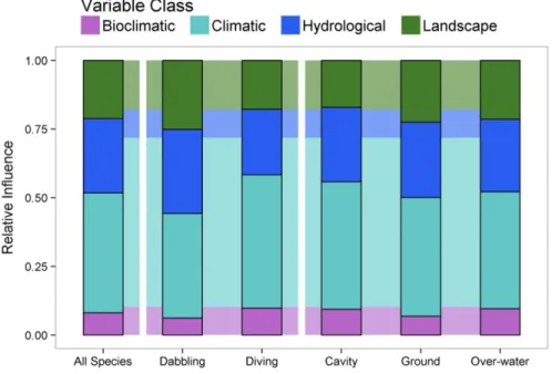
classes of environmental covariates: climatic, bioclimatic, hydrological, and landscape, and informally examine if their relative importances differ by feeding or nesting habit.

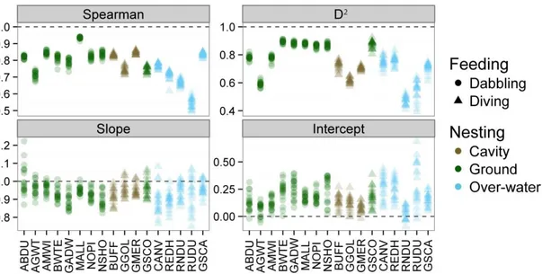
Table 1.1. Species and species groups included in this study, along with the feeding and nesting guild assigned to each. Guild classifications are based on Bellrose (1980), Johnsgard (2010), and Ehrlich et al. (1988).

Abbreviation Common Name Scientific Name Feeding Guild Nesting Guild

ABDU American Black Duck Anas rubripes Dabbling Ground

AGWT Green-winged Teal Anas crecca Dabbling Ground

AMWI American Wigeon Anas americana Dabbling Ground

BWTE Blue-winged Teal Anas discors Dabbling Ground

GADW Gadwall Anas strepera Dabbling Ground

MALL Mallard Anas platyrhynchos Dabbling Ground

NOPI Northern Pintail Anas acuta Dabbling Ground

NSHO Northern Shoveler Anas clypeata Dabbling Ground

BUFF Bufflehead Bucephala albeola Diving Cavity

GGOL Goldeneye species Bucephala clangula Diving Cavity

Bucephala islandica

GMER Merganser species Mergus merganser Diving Cavity

Mergus serrator Lophodytes cucullatus

GSCO Scoter species Melanitta americana Diving Ground

Melanitta fusca Melanitta perspicillata

CANV Canvasback Aythya valisineria Diving Over-water

REDH Redhead Aythya americana Diving Over-water

RNDU Ring-necked Duck Aythya collaris Diving Over-water RUDU Ruddy Duck Oxyura jamaicensis Diving Over-water

GSCA Scaup species Aythya affinis Diving Over-water

Aythya marila

Methods

Waterfowl Population Data

We obtained waterfowl count data from the Waterfowl Breeding Population and Habitat Survey (Smith 1995). Observers count adults of common waterfowl species seen within 200 m of fixed-wing aircraft flight transects. Within transects, counts are spatially assigned to “segments” of about 28.8 km (by 0.4 km width for a segment area of 11.2 km2_{). See Smith}

(36)

(1995), USFWS (2012a), Zimmerman et al. (2012) and the Thesis Annex for details on survey methodology.

Figure 1.1. Top: Survey strata and transects of the Waterfowl Breeding Population and Habitat Survey (WBPHS) in Canada. Bottom: Some major lakes, rivers, and ecoregions referred to herein. The orange colors depict the four ecoregions of the prairie-parkland. References to “prairies” denote the northwestern glaciated plains if confined to Canada, or the union of the two plains ecoregions when including the USA. We split the boreal region (Brandt 2009) along the Ontario-Manitoba border to facilitate discussion of regional variation in waterfowl abundances.

(37)

We modelled segment-level counts of Total Indicated Pairs from the Canadian portion of the WBPHS survey area (2273 segments). Total Indicated Pairs is an estimate of the number of pairs present based on the raw counts of actual pairs and lone males detected, taking into account species-specific life history (Dzubin 1969, Smith 1995, USFWS 2012a). We used 15 years of data from 1995-2010; data from 2007 were excluded due to a deviation in that year from the usual survey design (Silverman 2011). We used this temporal subset to capture a relatively static, recent, and representative sample of waterfowl counts. Only some segments of the ESA were sampled in some years, if at all, prior to 1995; restricting the analyzed sub-sample to after this year increases temporal and spatial density within the analyzed dataset.

We created 17 species abundance models, 13 for individual species and four for species that are grouped within the survey protocol (goldeneye, mergansers, scoters, and scaup; Table 1.1). These four groups are referred to as species hereafter. To explore how characteristics of fitted models might vary with life-history, species were assigned feeding and nesting guilds (Table 1.1) following Bellrose (1980) and Johnsgard (2010). We classified the merganser group as “cavity nesting”, despite the Red-breasted Merganser (Mergus serrator) being a ground nester (Titman 1999), to reflect the more specialized nesting habit of the other two species in the group.

Environmental Data

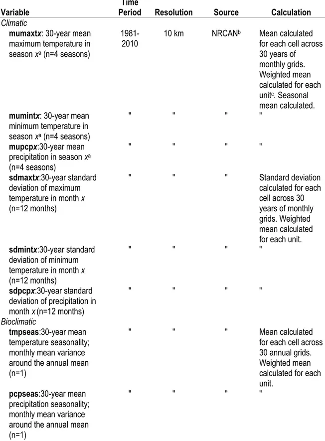
We selected environmental predictor variables based on previous studies of waterfowl habitat selection (Horn et al. 2005, Paszkowski and Tonn 2006, Suhonen et al. 2011) and songbird distribution (Cumming et al. 2014, Stralberg et al. 2015). Selection criteria included a priori hypotheses on likely ecological relationships (Mac Nally 2000, Barry and Elith 2006, Wenger and Olden 2012), constrained by availability and coverage. Where possible, we prioritized variables with more direct and likely causal relationships with waterfowl abundance, though proxy or indirect variables (Austin 2002b) were used in many cases. We used a total of 78 climatic, bioclimatic, landscape, and hydrological predictor variables (Table 1.2).

(38)

Table 1.2. Environmental variables used in Boosted Regression Trees of waterfowl abundance.

Variable Period Time Resolution Source Calculation

Climatic

mumaxtx: 30-year mean maximum temperature in season xa_{(n=4 seasons)}

1981-2010 10 km NRCAN

b _{Mean calculated}

for each cell across 30 years of

monthly grids. Weighted mean calculated for each unitc_{. Seasonal}

mean calculated. mumintx: 30-year mean

minimum temperature in season xa_{(n=4 seasons)} " " " " mupcpx:30-year mean precipitation in season xa (n=4 seasons) " " " " sdmaxtx:30-year standard deviation of maximum temperature in month x (n=12 months) " " " Standard deviation calculated for each cell across 30 years of monthly grids. Weighted mean calculated for each unit. sdmintx:30-year standard deviation of minimum temperature in month x (n=12 months) " " " " sdpcpx:30-year standard deviation of precipitation in month x(n=12 months) " " " " Bioclimatic tmpseas:30-year mean temperature seasonality; monthly mean variance around the annual mean (n=1)

" " " Mean calculated for each cell across 30 annual grids. Weighted mean calculated for each unit.

pcpseas:30-year mean precipitation seasonality; monthly mean variance around the annual mean (n=1)

(39)

temprange:30-year mean temperature annual range; difference between the maximum of the warmest month and the minimum of the coldest month (n=1)

" " " "

wetmonth:30-year mean of precipitation in wettest month (n=1)

" " " "

drymonth: 30-year mean of precipitation in driest month (n=1)

" " " "

mugrow: 30-year mean of growing season length; number of days above 5°C (n=1)

" " " "

sdgrow: 30-year standard deviation of growing season length (n=1)

" " " "

gpp: 7-year average gross primary productivity, in gC/m2_/yrd_(n=1) 2000-2006 1 km Terradynamic Numerical Simulation Groupe Weighted mean calculated for each unit.

Landscape

lcc.C.i: Proportion of area covered by land cover class i, described in Table 1.3 (n=12 cover classes).

Static

(2005) 250 m Centre for Remote Sensingf 𝐶𝑖 / 𝐶𝑡 Ci = Count of cells of land c class i within unit Ct = Total cell count in unit sdi: Shannon Diversity Index

for land cover classes (n=1) " " " ∑(𝑃𝑖 ∗ ln(𝑃𝑖))

𝑚 𝑖=1 ) m = number of land cover types Pi= proportion of area covered by land cover type topo: Index of topographic

ruggedness; calculated as coefficient of variation from a DEM (n=1) Static (2000 and 1993-1 km Integrated Remote Sensing Studiog Weighted mean calculated for each unit.

(40)

Hydrological

cmi: 30-year average climate moisture index; cm

precipitation – cm potential evaporation per yearh _(n=1)

1961-1990 10 km NRCAN Weighted mean calculated for each unit.

hwlwetland/hwlwater: Proportion of area covered by open water or wetlandsi

(n=2 classes) Static (2000 and 2009) 25 m Ducks Unlimited Canada Count of water or wetland cells within each unit,

expressed as a proportion of total number of cells within unit. streamlength: Total length

of streams in m stream/km2 area (n=1) Static (created from data from 1994-2010) 1:10,000-1:50,000 Hydrology National Networkj Length of all streams, divided by unit area (to standardize).

wbdens: Density of water bodies in unit neighbourhood (n=1)

" " " Number of water bodies intersected by unit, divided by unit area (to standardize). muareawbods: Mean size of

water bodies in unit neighbourhood (n=1)

" " " Mean area of water bodies intersected by unit, divided by unit area (to standardize). shorelength: Length of shoreline in km shoreline/km2 area (n=1) " " " Total shoreline (perimeter of water bodies) contained within unit, divided by unit area (to standardize). shorecx: Shoreline

complexity (area-weighted shape index for water bodies in unit neighbourhood) (n=1)

" " " Ratio of water body perimeter to area measured against a circle standard. Mean across water bodies weighted by area of water body within unit.

(41)

a_{Seasons as follows: Winter: Dec, Jan, Feb; Spring: Mar, Apr, May; Summer: Jun, Jul,}

Aug; Autumn: Sept, Oct, Nov.

b_{McKenney, D. W., M. F. Hutchinson, P. Papadopol, K. Lawrence, J. Pedlar, K. Campbell,}

E. Milewska, R. F. Hopkinson, D. Price, and T. Owen. 2011. Customized spatial climate models for North America. Bulletin of the American Meteorological Society 92:1611– 1622.

c_{unit = segment buffer or grid cell (see Methods: Environmental data).}

d _{from the MOD17A3 product. Zhao, M., F. A. Heinsch, R. R. Nemani, and S. W. Running.}

2005. Improvements of the MODIS terrestrial gross and net primary production global data set. Remote Sensing of Environment 95:164–176.

(http://www.ntsg.umt.edu/project/mod17)

e _{NTSG at the University of Montana. (http://www.ntsg.umt.edu/)}

f_{Canada Centre for Remote Sensing 2008. Land Cover Map of Canada 2005.}

(ftp://ftp.ccrs.nrcan.gc.ca/ad/NLCCLandCover/LandcoverCanada2005_250m/) 2008.

g_{Integrated Remote Sensing Studio.}

http://databasin.org/datasets/14d70746535e4be99aaf66595cc0b677

h _{Calculated from modified Penman-Monteith potential evapotranspiration. Hogg, E. H.}

1994. Climate and the southern limit of the western Canadian boreal forest. Canadian Journal of Forest Research 24:1835–1845.

i_{Jones, N. 2010. Hybrid Wetland Layer (Version 2.1) User Guide. Ducks Unlimited}

Canada.

j National Hydrology Network. 2007. Government of Canada. Available on Geobase. (http://www.geobase.ca/geobase/en/data/nhn/description.html)

Annual climatic variables and most bioclimatic indices were extracted from interpolated weather station data provided by Natural Resources Canada (McKenney et al. 2011). We calculated 30-year means of maximum and minimum monthly temperature, summarized to season, to capture the influence of precipitation through wetland conditions. We calculated 30-year standard deviations of monthly maximum temperature, minimum temperature, and precipitation as proxies for the probabilities of extreme events (Lynch et al. 2013, Cumming et al. 2014) Thirty year means of bioclimatic variables capture effects of seasonality in temperature and precipitation, the duration of the breeding season, and other factors (Table 1.2). Gross primary productivity was included as a proxy for food availability, both directly as plant food and indirectly through the provision of food for invertebrate prey.

(42)

We included variables for land cover to capture the influence of upland vegetation on waterfowl abundance and distribution, using the 250 m resolution Land Cover Map of Canada (Latifovic et al. 2008). The original 39 land cover classes were reclassified to 16 (Table 1.3). Proportional class areas were calculated per segment. Shannon’s diversity index was calculated from these land cover proportions as an index of habitat heterogeneity. Topographic ruggedness (Integrated Remote Sensing Studio 2010) was included to represent the influence of landform or terrain.

(43)

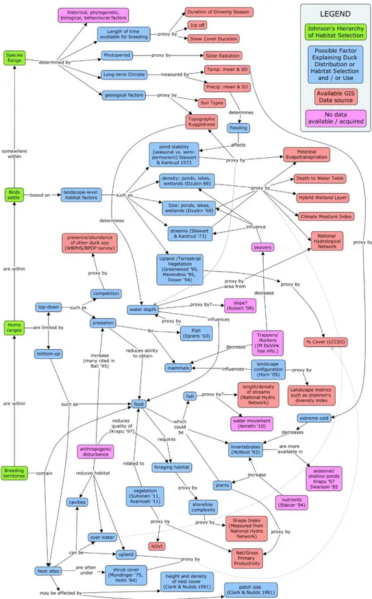
Figure 1.2. Conceptual map summarizing the rationale behind our variable selection. Where data sources (coral) were not available, proxie layers (pink) were used.

(44)

To measure the type and abundance of surface waters, we calculated the proportional area of wetlands (including swamps, marshes, bogs, and fens) and open water (including shallow open water and deeper water systems) in each segment, using Ducks Unlimited Canada's Hybrid Wetland Layer (Jones unpublished report). Shoreline length and complexity, stream length, and the density and mean size of water bodies were measured from the National Hydrology Network product (Natural Resources Canada 2007; Table 1.2). These variables were included to represent influences of size, depth, and shape of wetlands, as surrogates for availability of different foods for waterfowl.

All environmental variables were measured over a 1 km buffer around each segment, to account for imprecision in survey flight lines among years, and to capture the influence of local environmental conditions. Spatial analysis relied on the integration of raster and vector data in PostGIS 2.0 (Obe and Hsu 2011).

Table 1.3. Reclassification of Land Cover of Canada’s (2005) original 39 land cover classes to 16. The following classes were excluded to avoid duplication with other covariates or because of low values within the study area: burn (7), water (14), wetland/bog (15), and snow/ice (16).

Reclass

Name Reclass Number Original Class Name

High density

evergreen 1 Temperate or subpolar needle-leaved evergreen closed tree canopy Medium

density evergreen

2 Temperate or subpolar needle-leaved evergreen medium density, moss-shrub understory

Temperate or subpolar needle-leaved evergreen medium density, lichen-shrub understory

Low density

evergreen 3 Temperate or subpolar needle-leaved evergreen low density, shrub-moss understory Temperate or subpolar needle-leaved evergreen low density, lichen (rock) understory

Temperate or subpolar needle-leaved evergreen low density, poorly drained

Sparse needle-leaved evergreen, herb-shrub cover Deciduous 4 Cold deciduous closed tree canopy

Cold deciduous broad-leaved, low to medium density

Cold deciduous broad-leaved, medium density, young regenerating Mixed,

deciduous-dominated

5 Mixed cold deciduous - needle-leaved evergreen closed tree canopy Low regenerating young mixed cover

(45)

Reclass

Name Reclass Number Original Class Name

Mixed, evergreen-dominated

6 Mixed needle-leaved evergreen - cold deciduous closed tree canopy Mixed needle-leaved evergreen - cold deciduous closed young tree canopy

Mixed needle-leaved evergreen - cold deciduous, low to medium density

needle-leaved evergreen, low to medium density

Burn 7 Recent burns

Old burns

Shrubland 8 High-low shrub dominated Herb-shrub-bare cover Barren 10 Polar grassland, herb-shrub

Shrub-herb-lichen-bare Lichen-shrub-herb-bare soil Low vegetation cover Lichen barren

Lichen-sedge-moss-low Rock outcrops

Cropland 11 High biomass cropland Medium biomass cropland Low biomass cropland Crop/woodlan

d 12 Cropland-woodland

Urban 13 Urban and Built-up

Water 14 Water bodies

Mixes of water and land Wetland/bog 15 Herb-shrub poorly drained

Wetlands

Lichen-spruce bog Snow/Ice 16 Snow or ice

Statistical Methods

We built SAMs using Boosted Regression Trees (BRTs), a machine learning technique that combines the advantages of decision-tree analyses with boosting and bagging algorithms to improve predictive performance (Friedman et al. 2000, Friedman 2002). BRTs have several advantages: they detect important relationships from large sets of predictor variables; they accommodate the complex, non-linear relationships that often exist between species and habitat (Gaston 2003); they accommodate multi-way interactions among predictor variables; they are insensitive to outliers and transformations of the predictor variables (Elith et al. 2008); and show good predictive performance (Elith et al. 2006, 2008, Oppel et al. 2012).