HAL Id: in2p3-00022014
http://hal.in2p3.fr/in2p3-00022014
Submitted on 28 Jan 2021
HAL is a multi-disciplinary open access
archive for the deposit and dissemination of
sci-entific research documents, whether they are
pub-lished or not. The documents may come from
teaching and research institutions in France or
abroad, or from public or private research centers.
L’archive ouverte pluridisciplinaire HAL, est
destinée au dépôt et à la diffusion de documents
scientifiques de niveau recherche, publiés ou non,
émanant des établissements d’enseignement et de
recherche français ou étrangers, des laboratoires
publics ou privés.
Goodness-of-fit statistics and CMB data sets
M. Douspis, J. G. Bartlett, A. Blanchard
To cite this version:
M. Douspis, J. G. Bartlett, A. Blanchard. Goodness-of-fit statistics and CMB data sets. Astronomy
and Astrophysics - A&A, EDP Sciences, 2003, 410, pp.11-16. �10.1051/0004-6361:20030869�.
�in2p3-00022014�
A&A 410, 11–16 (2003) DOI: 10.1051/0004-6361:20030869 c ESO 2003
Astronomy
&
Astrophysics
Goodness–of–fit statistics and CMB data sets
M. Douspis
1,2, J. G. Bartlett
1,3, and A. Blanchard
11 Observatoire Midi-Pyr´en´ees, 14 Av. E. Belin, 31400 Toulouse, France
Unit´e associ´ee au CNRS (http://webast.ast.obs-mip.fr)
2 Astrophysics, Denis Wylkinson Building, Keble Road, Oxford OX1 3RH, UK
(http://www-astro.physics.ox.ac.uk)
3 APC, Universit´e Paris 7, 11 Pl. Marcelin-Berthelot, Paris Cedex 05, France (http://apc-p7.org/)
Received 25 September 2001/ Accepted 19 May 2003
Abstract. Application of a Goodness–of–fit (GOF) statistic is an essential element in parameter estimation. We discuss the computation of GOF when estimating parameters from anisotropy measurements of the cosmic microwave background (CMB), and we propose two GOF statistics to be used when employing approximate band–power likelihood functions. They are based on an approximate form for the distribution of band–power estimators that requires only minimal experimental information to construct. Monte Carlo simulations of CMB experiments show that the proposed form describes the true distributions quite well. We apply these GOF statistics to current CMB anisotropy data and discuss the results.
Key words.cosmology: cosmic microwave background – cosmology: observations – cosmology: theory
1. Introduction
Measurement of the cosmic microwave background (CMB) temperature anisotropies has proven to be one of the most powerful tools for estimating important cosmological param-eters (Netterfield et al. 2002; Pryke et al. 2002; Rubino-Martin et al. 2002; Sievers et al. 2002; Wang et al. 2002). The observed angular power spectrum shows the coherent peak structure expected in inflationary models, and fitting model curves to the data1 yields constraints on many parameters. This leads in particular to the conclusion that the geometry of space is flat (Lineweaver et al. 1997; de Bernardis et al. 2000; Hanany et al. 2000; Lange et al. 2000; Balbi et al. 2000). In terms of statistics, the procedure just described is one of pa-rameter estimation.
Parameter estimation proceeds via the identification of a best model (set of parameters) within a family of models, an evaluation of the quality of the fit and the construction of pa-rameter constraints. The method of maximum likelihood (ML), for example, is a useful, general procedure for finding a best–fit model. As a general rule, one must judge the quality of the fit before any serious consideration of parameter constraints. This requires the application of a Goodness–of–fit (GOF) statistic. Such a statistic is, usually, some scalar function of the data whose distribution may be calculated once given an underly-ing physical model and a model of the statistical fluctuations in
Send offprint requests to: M. Douspis,
e-mail: [email protected]
1 See http://webast.ast.obs-mip.fr/cosmo/CMB for an up–
to–date compilation.
the data. It is generally a function go f (d, T ) of both the data d and theory T , such that go f attains, for example, a minimum when d is generated by the theory T . It is defined in a “mono-tonic” way, in the sense that go f becomes larger as d gets “fur-ther” from a realization of T . The “significance” may then be defined as the probability of obtaining go f > go fobs. On this
basis, it permits a quantitative evaluation of the quality of the best model’s fit to the data: if the probability of obtaining the observed value of the GOF statistic (from the actual data set) is low (low significance), then the model should be rejected. Without such a statistic, one does not know if the best model is a good model, or simply the “least bad” of the family.
In this paper, we examine in some detail the issue of GOF when analysing anisotropy data on the cosmic microwave background. The vast majority of present analyses of the power spectrum data do not include proper GOF evaluations. The problem is particularly complicated by the fact that approxi-mate likelihood methods must be employed in order to process the large volume of data and to explore a significant part of parameter space. These methods usually rely on power spec-trum estimates, such as flat band–powers, extracted either from scan data, or from reconstructed sky maps. Because the power is quadratic in the temperature fluctuations, it is clear that these estimates are not Gaussian distributed. The traditional ap-proach of χ2 minimisation incorrectly assumes that power
es-timates are Gaussian distributed, something that can lead to a bias in determining the best model (e.g., Douspis et al. 2001a). For the same reason, the value of the reduced χ2 at the best
model does not retain its usual statistical meaning and may therefore not be simply used as a GOF statistic.
12 M. Douspis et al.: Goodness of fit in CMB Approximations to the band–power likelihood function that
permit more rigorous analyses have been proposed (Bond et al. 2000; Bartlett et al. 2001). The question remains, however, of how to correctly evaluate the GOF of the best model. Such an evaluation requires knowledge of the distribution of the power estimates, which is not necessarily the same as the likelihood function. Using the same approach as Bartlett et al. (2001; hereafter Paper I), we propose an ansatz for the distribution of band–power estimates and test it against Monte Carlo sim-ulations of certain MAX and Saskatoon data sets. The ansatz requires only minimal experimental information, and it appears to work well. We therefore use it to construct two GOF statis-tics, which we then apply to various ensembles of the present CMB data set.
2. Likelihood method
It is useful to begin with a discussion of GOF in the context of a complete likelihood analysis. Although computationally challenging (in fact, impossible for large data sets: Bond et al. 2000; Borrill 1999a,b), a likelihood approach is conceptually straightforward and our discussion serves to highlight certain important points. Such an analysis is in any case required for a small subset of data in order to test approximate methods (see, for example, Douspis et al. 2001a, hereafter Paper II).
Following the notation of Papers I and II, we write the like-lihood function as (we consider only Gaussian perturbations) L(−→Θ) ≡ Prob(−→d|−→Θ) = 1 (2π)Npix/2|C|1/2e −1 2→−d t ·C−1·→−d (1)
where C(−→Θ) is the correlation matrix (a function of the model parameters −→Θ and including a contribution from instrumental noise), and −→d is column vector listing the pixel values2. The
elements of −→Θ may be either the cosmological parameters, or a set of band–powers. Maximising the likelihood function over the parameters defines the “best model” corresponding to the parameters −→Θbest.
In the present situation, we are greatly aided by the Gaussian form of Eq. (1) in the data vector, −→d . Given the best
model, the most obvious GOF statistic is then clearly
go f = −→dt· ˜C−1· −→d (2)
where ˜C ≡ C(−→Θbest) is the correlation matrix evaluated at
the best model. For the Gaussian fluctuations we have as-sumed, this quantity follows a χ2distribution, with a number of
degrees–of–freedom (DOF) approximately equal to the number of pixels minus the number of parameters3.
2 These “pixels” may either be the simple pixels of a map, or
tem-perature differences, as given by, for example, MAX.
3 This recipe does not strictly apply in the present case, because
the parameters are non–linear functions of the data; it is nevertheless standard practice. In any case, the number of pixels is in practice much larger than the number of parameters.
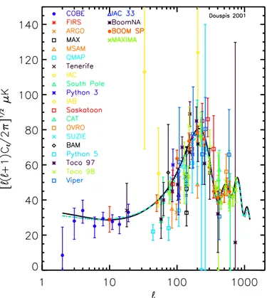
Fig. 1. Power spectrum plot of some actual CMB data.
3.
χ
2methodFor a variety of reasons (e.g., increased computational speed or inaccessible pixel data) most parameter estimations use power estimates, δT2, as their starting point, such as those shown in Fig. 1. A classic minimisation of χ2
χ2(−→Θ) = Nexp X n=1 δT obs n − δTn(−→Θ) σn 2 (3)
is commonly used to find −→Θbest and the best model, where
σn= σ+(σ−) if the model passes above (below) the data point. The obvious GOF statistic would then be the value of the χ2 evaluated at the minimum: go f = χ2(−→Θ
best). As already noted,
this whole procedure is inappropriate because power estimates do not follow a Gaussian distribution. It is of course true that if the number of contributing effective degrees–of–freedom4is large, a power estimate will closely follow a Gaussian; this, however, is never the case on the largest scales probed by a sur-vey. We shall see in the following that, for actual CMB data, the χ2 approach leads to quantitatively different results than
other, more appropriate GOF statistics. For future reference, we show the value of this classic χ2in Table 1.
4. Proposed approximation
To improve the χ2analysis, several authors have proposed
ap-proximations to the band–power likelihood functionL(δT) that may be constructed based on only minimal information about
4 Less than the number of original pixels by a factor depending on
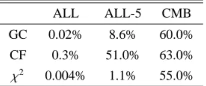
Table 1. Values of the GOF of the “best models” for each subset of
the actual data. GC is for “generalised χ2”, CF for the “characteristic
functions” technique and χ2for the classic χ2.
ALL ALL-5 CMB GC 0.02% 8.6% 60.0% CF 0.3% 51.0% 63.0% χ2 0.004% 1.1% 55.0%
the experimental set–up (Bond et al. 2000; Paper I). One then arrives at the likelihood as a function of cosmological parame-ters −→Θ with L[δT(−→Θ)]. Unfortunately, these approximate lihood functions do not retain the normalisation of the full like-lihood over pixels (Eq. (1)). This is a crucial point for GOF: we cannot deduce the quantity in Eq. (2) from the value of the approximate likelihood at its maximum.
An alternative way to build a GOF statistic would be from the expected distribution of power estimates, i.e., the distribu-tion of points in Fig. 4 around the model curve. Testing the observed dispersion of actual power points around the best–fit model against this expectation amounts to a GOF. The main difficulty in this approach is that we do not have an expres-sion for the distribution of ML power estimates. It is impor-tant to understand that this distribution is not the same as the band–power likelihood, whose maximum is used to find the es-timated power. In this section, we first motivate and then test an approximation to the distribution of ML power estimates.
4.1. Motivating an ansatz
Our approach will be the same as in Paper I, and the fol-lowing results thus apply when using the approximate band– power likelihood introduced therein. We motivated our likeli-hood approximation with an unrealistically simplified situation of Npixuncorrelated pixels and uniform noise (refered to
here-after as the simple picture). This suggested a functional form depending on two parameters, an effective number of degrees– of–freedom ν and a noise parameter β; in the simple picture, ν = Npix and β2 is the noise variance. These two parameters
could be found in realistic situations by adjusting to published flat–band confidence intervals (“errors”). The particular advan-tage of such a technique is that it permits an approximate like-lihood analysis based on rather rudimentary information often found in the literature; this is an important advantage for many first generation experiments. In this same spirit, we now pro-pose an ansatz for the ML band–power estimators.
For the simple picture (ν = Npix and β2 = noise variance),
we showed in Paper I that the ML band–power estimator, δT2, was a linear transform of a χ2N
pixrandom variable:
χ2
ν= ν
([δT ]2+ β2)
([δT (−→Θ)]2+ β2) (4)
where δT2(−→Θ) is the band–power of the underlying model. In
a realistic situation where ν and β are found from published power estimates, there is no a priori guarantee that this for-mula applies with the same values of ν and β. One is, of course,
tempted to suppose that the same values may in fact be used, at least approximatively. This hope forms the basis of our pro-posed ansatz for the band–power estimator distribution: P(δT2|−→Θ) ∝ Y(ν/2−1)e−Y/2
Y[δT2] ≡ ν ([δT ]
2+ β2)
([δT (−→Θ)]2+ β2)·
(5)
The underlying model band–power δT2(−→Θ) is in practice taken
to be the ML estimate. The essential spirit of our approach is that, knowing the flat–band estimates and the 68 and 95% confidence levels, one is able to reconstruct the entire likeli-hood function and (now) the probability distribution of the es-timate δTfb.
The only way to be sure that this proposed method actually works is by testing it against Monte Carlo simulations of some experiments before generalised it. We mention at least one rea-son for caution: the quantity ν represents an effective number of DOF, reduced from Npixby inter–pixel correlations,
applica-ble to the likelihood function; it is not at all clear that this same effective DOF applies equally well to the power estimator dis-tribution (as it does in the simple picture). In particular, note that since the same data where used to find the best–fit model, we might expect a reduction in DOF, something familiar from the classic reduced χ2 test. Here, however, we have no clear
idea of the reduction. Fortunately, the proposed method never-theless appears valid, as the following Monte Carlo simulations demonstrate it.
4.2. Testing the ansatz
We simulated many different data realizations of the MAX ID (Clapp et al. 1994) and Saskatoon (Netterfield et al. 1996) ex-periments in order to reconstruct the corresponding ML power estimator distribution. For example, we ran 30 000 realizations of MAX ID at a frequency of 3.5 cm−1in the following man-ner: we first compute the flat band–power and the one dimen-sional likelihood function for the actual observational data. Knowledge of the latter provided the value of the pair (ν, β). The maximum of the likelihood function gave us the “best model”, which was used to simulate pixels on the sky. In order to take into account all correlations, we simulated our pixels using the full pixel–pixel correlation matrix. We first computed the theoretical part of the correlation matrix evaluated for our “best model”. After diagonalization, we drew 30 000 realisa-tions of 21 pseudo–pixels from a Gaussian distribution centered on 0 and with the variances given by the eigenvalues. We re-constructed the “true” sky pixels using the transformation ma-trix (eigenvector mama-trix) and adding realizations of Gaussian noise (given by the known noise correlation matrix). We thus obtained 30 000 sets of 21 pixels, correlated and drawn accord-ing to the best model (δTfb = 57.3 µK). For each realization,
we derived the ML power estimate and build a histogram of its distribution.
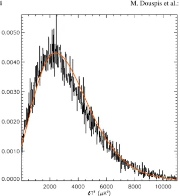
Figure 2 shows the resulting distribution for
MAX ID 3.5 cm−1. Overplotted in red as the smooth
curve is the ansatz Eq. (5) with the same values of (ν, β) as found from the likelihood function. We see that the proposed
14 M. Douspis et al.: Goodness of fit in CMB
Fig. 2. Distribution of the ML flat band–power estimator for
MAX ID 3.5 cm−1 found by Monte Carlo simulation. The smooth (red) curve is the approximation Eq. (5), which fits the distribution well.
approximate distribution is indeed a good representation of the true power estimator distribution.
The same kind of analysis was performed for the Saskatoon
K–band 3–point data, an altogether different observing
strat-egy. Once again, the approximation fitted the distribution to high accuracy. On the basis of these agreements, we will now adopt the proposed form in Eq. (5) as a good representation of the distribution of ML band–power estimators.
4.3. From probability function to GOF
On the basis of the distribution Eq. (5), we now construct two GOF statistics. The goal is to define a scalar quantity, go f , that measures the scatter of points around a given model and whose distribution is known under the hypothesis that this model rep-resents the “truth” (the null hypothesis). An improbable value of go f would indicate that there is a problem.
Both constructions assume that the band–powers are in-dependent. This of course is not strictly true, but generally speaking published band–powers do not have strong statisti-cal correlations; for example, the residual correlation between the Saskatoon bands is at a level of∼10%. Calibrations errors, on the other hand, do induce important band–band correlations. As already mentioned, the present work does not include cal-ibration errors, and any “bad fit” indicated by our GOF tests could indicate either a false model, or that calibration errors are important. Our aim here is to show the ability of a proper GOF to identify problems with CMB power data fits, and to demonstrate the advantage of the two proposed GOF statistics on the naive and inappropriate classic χ2.
4.3.1. Generalized
χ
2For each band–power i, consider the variables αi defined as follows: Z αi −∞ 1 √πexp(−x2/2)dx = pi (6) where pi ≡ RδT2 i −β2 i P
i(δT2|−→Θ)dδT2 is calculated using Eq. (5). The αi are thus Gaussian random variables with zero mean and a variance of unity. Hence, the sum go f = PNexp
1 α
2 i fol-lows a χ2 distribution with N
band DOF and provides a handy
GOF statistic.
4.3.2. Characteristic functions
Another way to define a GOF statistic for a fit to Nband power
points relies on the following property of characteristic func-tions: the characteristic function for the sum of independent
random variables is given by the product of the individual
char-acteristic functions. Given the Nband random variables Yi and
their probability distributionsPi(Eq. (5)), we calculate the dis-tribution of the random variable z≡PiYi, which will represent the goodness of fit, as follows: for each Yi we can compute the corresponding characteristic functionΦi(k). Then using the property cited above, we can construct the characteristic func-tionΦz(k) of the variable z byΦz(k) = Φ1(k)...ΦNband(k). The
probability distribution function of z,F (z), is then given by the inverse Fourier transform ofΦz(k). This approach is particu-larly straightforward in our case because the probability func-tion given in Eq. (5) is just a χ2law with ν
iDOF, whose char-acteristic functionΦi has an analytic form. Multiplication of the individual characteristic functions thus gives an analytical expression whose inverse Fourier transform is itself a χ2
distri-bution in z, with ν=PνiDOF: F (z) = zν/2e−z/2 with z= X i Yi and ν= X νi
The variable go f = z is thus (another) χ2–distributed quantity
that provides a useful GOF statistic.
5. “The good, the bad and the GOF” or Are CMB fluctuations consistent with a Gaussian distribution?
5.1. Application
In this section we apply each of the above GOF statistics to the CMB data set shown in Fig. 1; note that this does note include the most recent BOOMERanG, MAXIMA and DASI results. Adding these new data will essentially results in reduc-ing the “χ2” distributed go f values without changing
drasti-cally the results presented in this section. Our overall approach is as described in Le Dour et al. (2000, hereafter Paper III) and Douspis et al. (2001a), where we used the likelihood ap-proximation given in Paper I to find the best model. We con-sider three combinations of data: Data set 1 contains all points
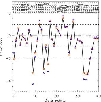
Fig. 3. Individual νi(red squares) and χ2 (blue triangles) for a subset
of the data plotted in Fig. 1.
(ALL)5; set 2 consists of all the data minus the Python 5 results
(Coble et al. 1999) (ALL-5); and set 3 combines just COBE (Tegmark & Hamilton 1997), MAXIMA (Hanany et al. 2000) and BOOMERanG (de Bernardis et al. 2000) (CMB). The best model for each data set will be referred to as BMALL, BMALL−5,
BMCMB. A summary of the various GOF statistics for these
models is given in Table 1; the lines are labelled by GC for “generalised χ2”, CF for “characteristic functions”, and “χ2” for the classic χ2of Eq. (3)6.
For GC technique, the go f is directly equivalent to the ab-solute value of a χ2. To convert this into percentage, we need to
know the DOF The latter is given in our case by the number of experiments taken into account in each set minus the number of free cosmological parameters.
For the CF technique, the percentage given in Table 1 is obtained by integrating the probability distribution function f of ZYfrom infinity to Zobs=PNisetZi2where Nsetis the number
of experiments in each set.
Figure 4 summarises the results given by our CF test on both data sets 1 and 2. The line gives the function to integrate and the shaded part is the integrated part corresponding to the numbers given in Table 1. The solid (blue) line and shaded part correspond to data set 1, and the dashed (red) line and arrow to data set 2.
5 Actually, we noticed that our approximation fails to recover the
MC simulations for upper limits. For this reason we do not include them in our analysis.
6 We noticed that σ
iis given different definitions in the literature.
When considering the evaluation of the GOF using each definition, we found that the value of the GOF is quite sensitive to the definition of σi. We consider in this paper the technique giving the best value of
the GOF.
Fig. 4. Results of the GOF for each subset given by our CF test. The
values of the GOF with the characteristic function technique are given by the blue shaded part for ALL subset and the red arrow for the ALL-5 subset.
5.2. Discussion
The first remark to be made based in Table 1 is that the com-plete data set (set 1) is inconsistent with a Gaussian sky fluc-tuations, according to all three techniques; the GC method, for example, excludes this hypothesis at more than 99.99%. This means in particular that it is not appropriate to search cosmo-logical constraints, because the whole class of models consid-ered is ruled out. This could be due to several effects, in partic-ular the fact that we do not include calibration uncertainties in our analysis.
The situation is different if we remove Python 5 (set 2) from the analysis. In this case, our two evaluations of the GOF (GC and CF) both accept the hypothesis of Gaussian sky fluctu-ations. In contrast, the classic (but inappropriate) χ2 statistic marginally excludes such hypothesis. Figure 3 illustrates the difference between our GC method and the classic χ2, data point by data point (for a subset of data set 1). Triangles show individual χ2values, while boxes correspond to the νidefined in Sect. 3. We see that the classic χ2 overpenalizes the fit for outliers, a conclusion already noted in Paper II.
Finally, we can see that all three methods accept the Gaussian hypothesis as a good representation to the COBE, MAXIMA and BOOMERanG data (set 3).
6. Conclusion
We have discussed three different ways of estimating the GOF to CMB band–powers. A GOF statistic is a key element of any parameter estimation study, and a good fit must be in-sured before considering parameter constraints. The classic χ2
GOF statistic is not rigorously applicable to power spectrum data, because power estimates are not Gaussian distributed quantities. We propose instead two alternative GOF statistics based on an approximation to the distribution of power esti-mators. This approximation was motivated by the same kind
16 M. Douspis et al.: Goodness of fit in CMB of arguments presented in Paper I for the likelihood function.
The distribution of a power estimator is a different quantity than the likelihood function used to define the estimator. We tested the approximation presented here against Monte Carlos simulations of CMB observations and found that it reproduced well the distribution of the maximum likelihood band–power estimator.
We then constructed two different GOF statistics, whose distributions were found using the approximate power estima-tor distribution. With the same, rather minimal information re-quired to build the likelihood approximation (Paper I), we are now also able to develop a GOF statistic to test the quality of the maximum likelihood model to a set of band–power data, thereby allowing a complete statistical analysis of anisotropy data from diverse observations. The method is limited by the fact that we are unable to account for correlations between band–powers; this, however, is not a serious restriction, as these correlations are usually rather unimportant for the final results based on current data sets.
In applying this approach to a set of band–power data of Fig. 1 we found that the “best model” obtained is in fact a bad fit. In other words, the data are unlikely to have been drawn from a Gaussian distribution represented by such a model. The fit becomes acceptable if we exclude the Python 5 points from the analysis, according to our GOF statistics. This is most likely due to the fact that we do not account for calibration errors, and so the bad fit probably just indicates that the adopted calibration is incorrect. It is interesting to note that, even with Python 5 removed, the classic χ2still marginally rejects the best fit. We
traced this behaviour to the fact that this method over weights the importance of “outliers”.
The important cosmological conclusion is that this CMB data set (excluding Python 5, due to our inability to ac-count for calibration errors) is consistent with Gaussian sky fluctuations drawn from the best–fit inflationary model.
A final remark concerns the possibility offered by the de-velopment of an approximated distribution function of the es-timators. In the application of current Monte Carlo methods for C`’s extraction (e.g. Szapudi et al. 2000, MASTER: Hivon et al. 2001), the estimator distribution is a natural output. The likelihood function needed in parameter estimations is however unknown. The present study suggests that we could reconstruct the likelihood function directly from the estimator distribution. The two parameters (ν and β) can be fitted on the estimator distribution and then used in the approximated likelihood func-tion of Bartlett et al. (2001). Consequently one is then able to reconstruct all the likelihood function and to perform a proper parameter estimation.
Acknowledgements. M.D. would like to thank Nabila Aghanim for
useful comments and corrections.
References
Balbi, A., Ade, P., Bock, J., et al. 2000, ApJ, 545, L1
Bartlett, J. G., Blanchard, A., Le Dour, M., Douspis, M., & Barbosa, D. 1998a, in Fundamental Parameters in Cosmology, Moriond Proc., ed. J. Trˆan Thanh Vˆan, et al. (Paris, France: ´Editions Fronti`eres) [astro-ph/9804158]
Bartlett, J. G., Blanchard, A., Douspis, M. & Le Dour, M. 1998b, to be published in Evolution of Large–scale Structure: from Recombination to Garching (Munich, Germany) [astro-ph/9810318]
Bartlett, J. G., Blanchard, A., Douspis, M., & Le Dour, M. 2000, Astrophys. Lett. Comm., 37, 321
Bartlett, J. G., Douspis, M., Blanchard, A., & Le Dour, M. 2000, A&AS, 146, 507 (BDBL)
Bond, J. R., Jaffe, A. H., & Knox, L. 2000, ApJ, 533, 19
Bond, J. R., & Jaffe, A. H. 1998, in Philosophical Transactions of the Royal Society of London A, Discussion Meeting on Large Scale Structure in the Universe, Royal Society, London, March 1998, [astro-ph/9809043]
Borrill, J. 1999a, in 3K Cosmology, AIP Conf. Proc., 476, 277, ed. L. Maiani, et al., [astro-ph/9903204]
Borrill, J. 1999b, in Proc. of the 5th European SGI/Cray MPP Workshop [astro-ph/9911389]
Clapp, A. C., Devlin, M. J., Gundersen, J. O., et al. 1994, ApJ, 433, L57
Coble, K., Dragovan, M., Kovac, J., et al. 1999, ApJ, 519, L5 de Bernardis, P., Ade, P. A. R., Bock, J., et al. 2000, Nature, 404, 955 Dodelson, S., & Knox, L. 2000, Phys. Rev. Lett., 84, 3523
Douspis, M., Bartlett, J. G., Blanchard, A. & Le Dour, M. 2001a, A&A, 368, 1
Douspis, M., Blanchard, A., Sadat, R., Bartlett, J. G., & Le Dour, M. 2001b, A&A, 379, 1
Efstathiou, G., Bridle, S. L., Lasenby, A. N., Hobson, M. P., & Ellis, R. S. 1999, MNRAS, 303, L47
Hanany, S., Ade, P., Balbi, A., et al. 2000, ApJ, 545, L5
Hancock S., Rocha G., Lasenby, A. N., & Gutierrez, C. M. 1998, MNRAS, 294, L1
Hivon, E., G´orski, K. M., Netterfield, C. B., et al. 2002, ApJ, 567, 2 Knox, L., &, Page, L. 2000, Phys. Rev. Lett., 85, 1366
Lahav, O., & Bridle, S. L. 1999, Evolution of Large Scale Structure: From Recombination to Garching, 190
Lange, A. E., Ade, P. A., Bock, J. J., et al. 2001, Phys. Rev. D, 63, 42001
Lasenby, A. N., Bridle, S. L., & Hobson, M. P. 1999, to be pub-lished in The CMB and the Planck Mission (Spain: Santander) [astro-ph/9901303]
Le Dour, M., Douspis, M., Bartlett, J. G., & Blanchard, A. 2000, A&A, 364, 369
Lineweaver, C., Barbosa, D., Blanchard, A., & Bartlett, J. G. 1997, A&A, 322, 365
Lineweaver, C. H., & Barbosa, D. 1998a, A&A, 329, 799 Lineweaver, C. H., & Barbosa, D. 1998b, ApJ, 496, 624 Lineweaver, C. H. 1998, ApJ, 505, 69
Netterfield, C. B., Devlin, M. J., Jarolik, N., Page, L., & Wollack, E. J. 1997, ApJ, 474, 47
Netterfield, C. B., Ade, P. A. R., Bock, J. J., et al., 2002, ApJ, 571, 604 Pryke, C., Halverson, N. W., Leitch, E. M., et al. 2002, ApJ, 568, 46 Rubino-Martin, J. A., Rebolo, R., & Carreira, P. 2003, MNRAS, 341,
1084
Szapudi, I., Prunet, S., Pogosyan, D., Szalay, A. S., & Bond, J. R. 2001, ApJ, 548, L115
Sievers, J. L., Bond, J. R., Cartwright, J. K., et al. 2002, ApJ, submitted [astro-ph/0205387]
Tegmark, M., & Hamilton, A. 1997 [astro-ph/9702019] Tegmark, M., & Zaldarriaga, M. 2000a, ApJ, 544, 30
Tegmark, M. & Zaldarriaga, M. 2000b, Phys. Rev. Lett., 85, 2240 Wang, X., Tegmark, M., & Zaldarriaga, M. 2002, Phys. Rev. D, 65,
123001
Webster, A. M., Bridle, S. L., Hobson, M. P., et al. 1998, ApJ, 509, L65