HAL Id: ird-00392195
https://hal.ird.fr/ird-00392195
Submitted on 5 Jun 2009
HAL is a multi-disciplinary open access
archive for the deposit and dissemination of
sci-entific research documents, whether they are
pub-lished or not. The documents may come from
teaching and research institutions in France or
abroad, or from public or private research centers.
L’archive ouverte pluridisciplinaire HAL, est
destinée au dépôt et à la diffusion de documents
scientifiques de niveau recherche, publiés ou non,
émanant des établissements d’enseignement et de
recherche français ou étrangers, des laboratoires
publics ou privés.
Modeling annual production and carbon fluxes of a large
managed temperate forest using forest inventories,
satellite data and field measurements
G. Le Maire, H. Davi, Kamel Soudani, C. François, Valérie Le Dantec, E.
Dufrene
To cite this version:
G. Le Maire, H. Davi, Kamel Soudani, C. François, Valérie Le Dantec, et al.. Modeling annual
production and carbon fluxes of a large managed temperate forest using forest inventories, satellite
data and field measurements. Tree Physiology, Oxford University Press (OUP): Policy B - Oxford
Open Option B, 2005, 25, pp.859-872. �ird-00392195�
Summary We evaluated annual productivity and carbon fluxes over the Fontainebleau forest, a large heterogeneous for-est region of 17,000 ha, in terms of species composition, can-opy structure, age, soil type and water and mineral resources. The model is a physiological process-based forest ecosystem model coupled with an allocation model and a soil model. The simulations were done stand by stand, i.e., 2992 forest manage-ment units of simulation. Some input parameters that are spa-tially variable and to which the model is sensitive were calculated for each stand from forest inventory attributes, a net-work of 8800 soil pits, satellite data and field measurements. These parameters are: (1) vegetation attributes: species, age, height, maximal leaf area index of the year, aboveground bio-mass and foliar nitrogen content; and (2) soil attributes: avail-able soil water capacity, soil depth and soil carbon content. Main outputs of the simulations are wood production and car-bon fluxes on a daily to yearly basis. Results showed that the forest is a carbon sink, with a net ecosystem exchange of 371 g C m– 2year– 1. Net primary productivity is estimated at 630 g C m– 2year– 1over the entire forest. Reasonably good agreement was found between simulated trunk relative growth rate (2.74%) and regional production estimated from the National Forest Inventory (IFN) (2.52%), as well as between simulated and measured annual wood production at the forest scale (about 71,000 and 68,000 m3year– 1, respectively). Results are discussed species by species.
Keywords: CASTANEA process-based model, Fontainebleau forest, NEE, remote sensing, soil carbon, spatialization.
Introduction
There are two challenges in modeling forest production: cou-pling forestry knowledge and process-based models, and scal-ing up from the stand to the regional scale. Couplscal-ing the mech-anistic approach based on ecophysiological rules with empiri-cal forestry knowledge provides a means to improve the
predictions of forest production under changing environmen-tal conditions (Makela et al. 2000). Early forest production models focused on forestry and yield prediction. These models used empirical rules based on large data sets from field experi-ments (Schober 1975, Dhote 1991) and could reproduce tree growth over a century, assuming no climatic trend, according to species, forest management and age of planting. They are not designed, however, to predict seasonal and inter-annual variations in tree growth and stand biomass increment and do not account for effects of global climatic change. Recently de-veloped process-based forest ecosystem models couple water and carbon exchange between vegetation and atmosphere. Some of these models also consider litter and soil mineraliza-tion processes. These models are designed to predict soil or-ganic matter dynamics and net ecosystem exchange of CO2 (NEE) (Baldocchi and Harley 1995, Hoffmann 1995, Kirsch-baum 1999). Although most of these models were developed to study and quantify water and carbon fluxes, they are now used for productivity assessment on year to century time scales, in the context of climate change (He et al. 1999, Makela et al. 2000, Landsberg 2003). These model simulations are in good agreement with actual measurements of carbon fluxes between the ecosystem and the atmosphere that have been measured in several forest stands by the eddy covariance tech-nique (Running et al. 1999, Kramer et al. 2002, Law et al. 2002).
The coupling between forestry and ecophysiological mod-els should first be done atthe stand scale, because this is the scale at which the process-based models are evaluated (both by aboveground wood production and flux measurements). The second objective is to scale up these coupling models. It is important to assess forest production at regional and global scales. Myneni et al. (2001) have found that the wood biomass of northern forests is probably a main sink of the annual anthropogenic input of CO2. The regional scale also allows the parameterization and the evaluation of the models and is an in-teresting scale for evaluating global carbon models.
ures, please send a high quality print of the revised figure(s). If this proof is returned by fax, please avoid writing in the outer 1 cm of the page, attach a typewritten list of changes and mail the original. Thank you.
Tree Physiology 25, 000–000
© 2005 Heron Publishing—Victoria, Canada
Modeling annual production and carbon fluxes of a large managed
temperate forest using forest inventories, satellite data and field
measurements
GUERRIC LE MAIRE,
1,2HENDRIK DAVI,
1KAMEL SOUDANI,
1CHRISTOPHE FRANÇOIS,
1VALÉRIE LE DANTEC
3and ERIC DUFRÊNE
11Laboratoire Écologie, Systématique et Évolution (ESE), CNRS & Université Paris Sud, Bât. 362, 91405 Orsay, France 2Corresponding author (guerric.le-maire@ese.u-psud.fr)
3Centre d’Études Spatiales de la Biosphère (CESBIO), 18 avenue Édouard Belin, BPI 2801, 31400 Toulouse Cedex 9, France
Few attempts have been made at spatialization of process-based forest modelsat the regional scale. These models con-tain numerous parameters, making their application difficult at regional or larger scales because of the large amount of data required for model parameterization. Combined remote sens-ing and geographic information systems (GIS) tools provide new approaches for scaling up processes from the stand to re-gional or larger scales (Plummer 2000). Ditzer et al. (2000) presents such a study for a 55,000 ha tropical rain forest using the process-based forest growth model Formix 3-Q. That model, however, cannot account for the effects of climate change; photosynthesis is empirically based; and the model does not simulate soil water balance, soil carbon fluxes and heterotrophic respiration. Nevertheless, the model has proved useful for studies on allometry and forest management. We are interested in the Formix 3-Q modeling study because applica-tion of the model over the whole forest relies on the use of a GIS database that includes forest inventory data and aerial photographs.
In the present work, we used and parameterized a detailed process-based model to simulate, at a regional scale, the pro-ductivity and carbon budget of a large, managed temperate for-est, characterized by high heterogeneity in species composi-tion, tree age, canopy structure, soil type and water and mineral resources. Our approach was to use local measure-ments (large stand-scale database) and simulations performed stand by stand over the whole forest with a process-based eco-system model. A distinctive feature of the study was that it linked forest inventories, soil inventories, satellite data and field measurements to produce a precise parameterization of the model and thus a precise quantification of forest carbon fluxes and productivity. This work is an essential first step to predicting both inter-annual and long-term climate effects on forest carbon balance at the regional scale.
Materials and methods
Model description
CASTANEA is a physiological multilayer process-based model designed to predict the carbon balance of an even-aged, monospecific deciduous forest stand. The main output vari-ables are: (1) leaf area index (LAI), standing biomass, soil car-bon content and water content, which are state variables; and (2) canopy photosynthesis, maintenance respiration, growth of organs, growth respiration, soil heterotrophic respiration, tran-spiration and evapotrantran-spiration, which are flux density vari-ables (Davi 2004, Dufrêne et al. (2005), Modeling carbon and water cycles in a beech forest. Part I: Model description and uncertainty analysis on modeled NEE, in revision for Ecologi-cal Modeling, hereafter referred to as CASTA1).
The canopy is assumed to be horizontally homogeneous and vertically subdivided into a variable number of layers, each enclosing the same amount of leaf area (typically less than 0.2 m2m– 2). No variability between trees is assumed and so one “average” tree is considered representative of the stand. A discussion of this assumption, based on an uncertainty
analy-sis, is given in CASTA1.The species used for the simulations are the main species of the stand, which may lead to inaccura-cies in some cases, especially when mixed coniferous–decidu-ous stands are being considered. Tree structure is represented as a combination of foliage, stems, branches, coarse and fine roots. A carbohydrate storage compartment is also represented but not physically located in the model.
From incident radiation and photosynthetic characteristics of individual leaves, half-hourly rates of gross canopy assimi-lation and transpiration are calculated. Leaf nitrogen per unit area (Na; g N m– 2leaf) is calculated from measured leaf nitro-gen concentration (Nm; g N gDM
– 1
leaf), which is assumed to be constant inside the canopy, multiplied by leaf mass per area (LMA), which decreases exponentially inside the canopy. Photosynthetic capacity of leaves in different canopy positions is derived from leaf Na.
After subtracting maintenance respiration requirements, the remaining assimilates are allocated to the growth of various plant tissuesbased on priorities that vary with season. The al-location coefficients depend only on the species. Fine roots and storage compartments were estimated by inverting the model assuming a constant biomass (i.e., equilibrium) on a yearly basis. This calibration was carried out at three sites, two in eastern France and one in the Netherlands: in Hesse for beech (Barbaroux 2002, CASTA1), in Champenoux for oak (Barbaroux 2002) and in Loobos for Scots pine (Davi 2004). The allocation coefficient for coarse roots was calculated as-suming a constant ratio between coarse roots and trunks (coarse root:shoot ratio): a value of 0.2 was deduced from Cairns et al. (1997). Carbon allocation to aboveground wood is thus the resultant and is not calibrated, allowing us to use it as a validation output. An evaluation of this calibration in the Fontainebleau forest is given by Barbaroux (2002), and possi-ble age and fertility effects are discussed below. Phenological stages (e.g., budburst, end of leaf growth, start of leaf yellow-ing) and leaf growth depend on degree days. Maintenance res-piration depends on temperature and Nmof various organs, whereas growth respiration depends on the biochemical composition of organs.
The soil water balance sub-model includes three soil layers. The soil organic carbon sub-model (based on the Century model (Parton et al. 1987) and described in Epron et al. (2001)) separates soil organic carbon into three major compo-nents, which include active pools (live soil microbes plus mi-crobial products), slow pools (resistant plant material) and passive pools (soil stabilized plant and microbial material) pools. Carbon flow between pools is controlled by decomposi-tion rate and a microbial respiradecomposi-tion loss parameter, both of which depend on soil texture, soil water and temperature. A major uncertainty in the soil model is the initialization of the carbon pools. We based the initialization on an equilibrium hy-pothesis.
There are two main time steps in the model: half-hourly and daily. The simulation period typically ranges from days to years. Most variables including fluxes (light penetration, pho-tosynthesis, respiration, transpiration, rainfall interception, soil evaporation) are simulated half-hourly, whereas all the
Au: Please provide the full refer-ence for Dufrêne et al. (2005), including authors' names and vol-ume number.
state variables (organ biomass, soil and carbon water content) and some others (growth and phenology) are simulated daily. The model includes several species sub-models, accounting for the main species of France: Fagus sylvatica L., Quercus
robur L./Quercus petraea (Matt.) Liebl. and Pinus sylves-tris L. Other species sub-models may also be included (e.g., Quercus pubescens Willd., Quercus ilex L. and Pinus pinaster
Ait.).
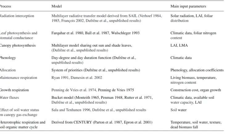
Input meteorological driving variables, either half-hourly or daily values, are global radiation, rainfall, wind speed, air hu-midity, temperature andatmospheric CO2concentration. A list of simulated processes and the original authors of the sub-models are given inTable1. A more complete description of the model, including equations, is given in CASTA1.
Most of the sub-models were tested and validated forF. syl-vatica with independent measurements of canopy
photosyn-thesis, autotrophic and heterotrophic respiration, NEE, wood and root growth, transpiration, soil water evaporation, rainfall interception and soil water status (Davi 2004, Davi et al. (2005), Modeling carbon and water cycles in a Beech forest. Part II: Validation for individual processes from organ to stand scale, in revision for Ecological Modeling, hereafter referred to as CASTA2). These measurements and validations were made at the Carboeuroflux Hesse flux-tower site (Granier et al. 2000) and are described in CASTA2. For the pine species, NEE, transpiration and evaporation fluxes were validated at the Loobos (Dolman 2002) and Le Bray Carboeuroflux sites (Berbigier et al. 2001). For the oak and beech species, model
validation was made on annual growth calculated from wood drill cores extracted at 22 stands in the Fontainebleau forest (13 oak stands, nine beech stands) (Barbaroux 2002, Davi 2004).
The CASTANEA model has about 200so-called parame-ters, most of which are constants: 15% are physical constants or regional parameters, and 65% are local-scale physical or biophysical constants describing the soil or the vegetation. These local-scale constants are dependent on tree species, but do not vary much from stand to stand (e.g., quantum yield). Fi-nally, 20% of the parameters are variable from one stand to an-other, even if the species is the same (e.g., stand age and LAI). In our study,most of these spatially variable parameters were determined or estimated.
The sensitivity of the model to the parameters has been studied on a yearly basis with a Monte-Carlo technique (CASTA1). Results have shown that the most sensitive param-eters are the photosynthetic paramparam-eters, soil water-holding capacity parameters, canopy structure parameters and phe-nology driving parameters.Parameters that are both sensitive and highly spatially variable include LAI, aboveground woody biomass (AWB), age, Nm, soil depth and available soil water capacity.
Study site
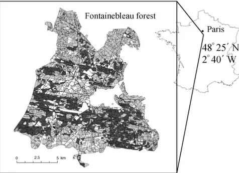
The Fontainebleau forest, located in the southeast of Paris (48°25′ N, 2°40′ E) extends over 17,000 ha (Figure 1), with a mean altitude of 120 m. The region is characterized by a
tem-Table 1. Description of the main processes simulated in the CASTANEA model, their sources and a short description of their main input parame-ters. Abbreviations: LAI = leaf area index; and LMA = leaf mass per area.
Process Model Main input parameters
Radiation interception Multilayer radiative transfer model derived from SAIL (Verhoef 1984, Solar radiation, LAI, foliar
1985, François 2002, Dufrêne et al., unpublished results) distribution
Leaf photosynthesis and Farquhar et al. 1980, Ball et al. 1987, Wulschleger 1993 Climatic data, foliar nitrogen
stomatal conductance content
Canopy photosynthesis Multilayer model sharing out sun and shade leaves, LAI, LMA
(Dufrêne et al., unpublished results)
Phenology Day-degree and day duration function (Dufrêne et al., Climatic data
unpublished results)
Allocation System of priorities (Dufrêne et al., unpublished results) Phenology, allocation coefficients
Maintenance respiration Ryan 1991, Damesin et al. 2002 Living biomass, temperature,
nitrogen content
Growth respiration Penning de Vries et al. 1974,Penning de Vries 1975 Construction cost, organ growth
Water fluxes Bucket model (Monteith 1965, Penman 1948, Rutter et al. 1971, Climatic data, available soil
Dufrêne et al., unpublished results) water capacity,LAI
Effect of soil water status Sala and Tenhunen 1996, Dufrêne et al., unpublished results Soilwater
on canopy gas exchange
Heterotrophic respiration and Derived from CENTURY (Parton et al. 1987, Epron et al. 2001) Temperature, soil water, texture,
soil organic matter cycle dead biomass fall
Au: Please provide the full refer-ence for Davi et al. (2005), including authors' names and vol-ume number. Au: The meaning of "shar-ing out sun and shade leaves" is un-clear. Please reword.
perate climate, with a mean annual temperature of 10.6 °C and a mean annual precipitation of 750 mm fairly well distributed throughout the year. This forest is actively managed by the French National Forest Office (ONF) and is divided into about 3600 management units. Regular forestry practices modify the structure and species composition of the forest stands. The for-est is composed of 38% oak (Q. robur/Q.petraea), 31% Scots pine (P. sylvestris) and 11% beech (F. sylvatica). The remain-ing 20% are other evergreen or deciduous species (5%) and sparsely wooded area (15%). These percentages are calculated with the main species of the stands, but only 10% of the forest is mixed deciduous–coniferous stands. Understory species are hornbeam (Carpinus betulus L.) and birch (Betula pendula Roth.). Most of the commercially exploited stands are located in areas of flat topography (plain and plateau), while slopes of the forest are mostly rocky and sparsely wooded. The soil is mainly sandy because of Stampian sand parent rock and depo-sition of windborne sands. These windborne sands are com-posed of Stampian sand mixed with loam and clay, and cover the whole forest to different depths (Robin 1993). The range in soil type varies widely, going from rendzine to podzol with various intermediate brunisols. Some parts of the forest also present hydromorphy, leading to gleyic soils.
The forest shows a great variety of stands, including the suc-cessive stage development: seedlings, thickets, sapling stands, pole stands, mature forest and seed tree stands. The range of species and soil types adds variability, so that the Fontaine-bleau forest captures major characteristics of a west paleoartic managed forest.
Available data set description
Forest inventory attributes Data arein a Geographical Infor-mation System built by the French National Forest Office in 1995. This GIS database contains a vectorized map of the
boundaries of the forest stands based on aerial photography in-terpretation and field surveys. The resulting delimited stands areeven-aged and homogeneous inspecies, structure, tree den-sity, spatial distribution of trees and silvicultural practices. The Fontainebleau forest is divided into 3635 stands, with a mean area of 5 ha. Figure 1 shows the stand boundaries with the main species. For each stand, the attributes determined by measure-ments and site surveys are: (1) stand structure including the dis-tribution of trees by age and size classes; (2) basal area of the stand estimated at a tree height of 1.30 m with a basal area relascope at three locations in the stand; (3) dominant tree height, estimated by eye; (4) the three main species reported in order of cover importance—their mean diameter class and per-cent cover over the stand estimated visually; (5) the age class of the three main species estimated visually, stump analysis, ar-chives references or wood drill core extraction, and the class in-tervals are 20 years for deciduous trees and 10 years for coniferous trees; and (6) other measured characteristics that were not used in our study.
Soil database The soil database was built by the French National Forest Office in 1995. It consists of about 8800 drilled pits evenly distributed over the forest (one every 2 ha). These measurements were done on a predefined spatial grid. Samples were obtained with a 2-m drill, and each description was made in the field. The attributes determined for each sample were soil type, humus type, underlying parent material and its depth if available, and for each horizon, the type, depth, texture, effer-vescence and pH. The nomenclature of soil and humus type was taken from Duchaufour (1982). The precision of the hori-zon thickness is less than 5 cm, and the total depth of the soil was reported when the drill blocked on the underlying parent material. Soil texture was determined as described by Baize (1988).
Figure 1. Forest map of the Fontaine-bleau forest (locatedsoutheast of Paris): Pinus sylvestris (dark gray), Quercus petraea/Q. robur (light gray), Fagus sylvatica (white) and other spe-cies (stipple).
Remotesensing data On July 10, 1995, SPOT satellite im-ages of the region were acquired in three spectral bands: green, red (R) and near infrared (NIR) and with a pixel size of 20 m. Images were rectified and geo-referenced using ground control points and integrated into the GIS database of Fontainebleau forest. Digital counts (gray tone) were converted to at-satellite (top of atmosphere) radiance (W m– 2 sr– 1 µm– 1) using the gains and the offsets contained in the image headers and then calibrated to scaled surface reflectance after atmospheric cor-rections using a Dark Object Subtraction approach (Song et al. 2001). The classical Normalized Difference Vegetation Index (NDVI) is calculated for each pixel of the image as: NDVI = (NIR – R)/(NIR + R).
Field measurements Field measurements were made be-tween 1994 and 2002 on 56 stands within the forest. The sam-pled stands represent the main species and a wide spectrum of ages, structures, soil compositions and tree densities. Most of the measurements in 1994 and 1995 were made during the Eu-ropean Multisensor Airborn Campaign (EMAC) organized by the European Space Agency (ESA), Ispra, Italy (Dufrêne et al. 1997). The measured variables were stand dendrometric char-acteristics: tree density, basal area, tree height, crown height, total biomass, trunk biomass and branch biomass, calculated as described by Proisy et al. (2000). In situ measurements of LAI were made with the Li-Cor LAI-2000 Plant Canopy Analyzer, from the end of June to mid-July 1995 under uniform diffuse sky on 41 of the 56 experimental stands. A detailed description and analysis of the spatial and temporal variability of LAI in the Fontainebleau Forest is given in Le Dantec et al. (2000). For leaf biochemical characteristics, sun and shade leaves were sampled to estimate leaf chlorophyll concentration, nitrogen concentration, LMA and leaf water content as described by Demarez et al. (1999). Stand age and annual wood increment of the stand were measured from wood drill cores as described by Barbaroux (2002).
Model parameterization
We tried to spatialize most of the parameters to which the model is sensitive and that have high spatial and temporal vari-ability among stands (see model description). For the other pa-rameters, we used the mean value for each species, based on field measurements (mostly in Fontainebleau) or from the literature.
Spatially determined parameterswere separated into tree parameters and soil parameters. Among the tree parameters, the most important were LAI, Nm(Wullschleger 1993), stand age (Table2), percentage of living biomass (Tables 1 and 2) and AWB. Among the soil parameters, we distinguished be-tween parameters describing soil water status and those de-scribing soil carbon status (Table 1). Analysis and spatiali-zation of the data sets were made with ESRI ArcGIS 8.1 soft-ware (Environmental Systems Research Institute, CA).
Species characteristics Species, age and height were
ex-tracted directly from the forest inventory. For each stand, the species considered is the main species of the stand as registered in the Fontainebleau forest GIS database (the case of mixed stands is discussed later). The age and the height of each stand were taken as the medians of the age and height classes for the main species.
Organ biomass and carbohydrate reserves Branch, trunk,
coarse root and carbohydrate storage biomass were derived from the total aboveground biomass of the stand(Figure2 and Table 2). Aboveground woody biomass (gDMha– 1or g C m– 2 based on the conversion factor 0.5) was estimated for the EMAC stands from field measurements and allometric equa-tions as described by Proisy et al. (2000). The product of basal area (BA) and dominant height (H) is linearly related to AWB. Two relationships were calibrated for deciduous and evergreen species (Le Dantec 2000):
AWB =aBA(H + b) (1)
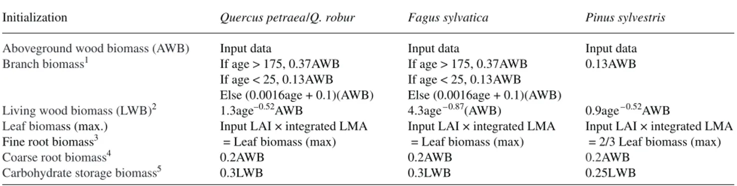
Table 2. Initialization of biomass compartments of the stands. Input data are leaf area index (LAI), aboveground wood biomass (AWB) and leaf mass per area (LMA).
Initialization Quercus petraea/Q. robur Fagus sylvatica Pinus sylvestris
Aboveground wood biomass (AWB) Input data Input data Input data
Branch biomass1 If age > 175, 0.37AWB If age > 175, 0.37AWB 0.13AWB If age < 25, 0.13AWB If age < 25, 0.13AWB
Else (0.0016age + 0.1)(AWB) Else (0.0016age + 0.1)(AWB)
Living wood biomass (LWB)2 1.3age–0.52AWB 4.3age– 0.87(AWB) 0.9age– 0.52AWB
Leaf biomass (max.) Input LAI × integrated LMA Input LAI × integrated LMA Input LAI × integrated LMA
Fine root biomass3 = Leaf biomass (max) = Leaf biomass (max) = 2/3 Leaf biomass (max)
Coarse root biomass4 0.2AWB 0.2AWB 0.2AWB
Carbohydrate storage biomass5 0.3LWB 0.3LWB 0.25LWB
1
Hatsch 1997.
2
Ceschia et al. 2002.
3
Vogt et al. 1987, Santantonio 1989, Bauhus and Bartsch 1996.
4 Cairns et al. 1997. 5 Barbaroux et al. 2003. Au: Please define SPOT. Au: What is LWB?
where a = 0.37 or 0.22 and b = –0.01 or 4.6, respectively, for deciduous (r2= 0.96, 35 stands) or coniferous stands (r2= 0.99, 13 stands).
Leaf area index, leaf biomass and fine root biomass Leaf
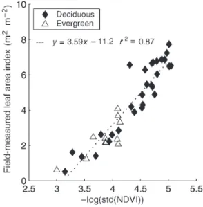
area indexwas estimated based on within-stand NDVI vari-ability (Davi 2004). For each stand, LAI was calculated based on an empirical relationship between ground-based LAI mea-surements and SPOT reflectance data calibrated over 40 stands (12 dominated by beech, 17 by oak and 11 by Scots pine) ( Fig-ure3).
The SPOT HRV satellite image was acquired in July 1995, which coincides with the period of maximum LAI of the stands (the model needs the maximal leaf area of the year and computes the increase and decrease in LAI in spring and au-tumn). After making the geometrical and atmospheric correc-tion procedures outlined above, NDVI was calculated for each image pixel. Then, based on the forest polygon coverage of forest stands, the standard deviation of NDVI was calculated for each stand. To avoid edge effects and overlapping pixels between stands, pixels located in a 20-m wide band along the polygon limits inside the stand were excluded. Stands com-posed of less than 25 pixels (1 ha) were not considered. For stands including more than 30 pixels, LAI was calculated as:
LAI = –3.59 log(std(NDVI)) – 11.22 (2)
where std(NDVI) is the standard deviation of the NDVI inside the stand (r2= 0.87, n = 40).
The remotely sensed LAI obtained from Equation 2 is underestimated in coniferous stands because of clumping of needles, branches and trees. To correct for this clumping, the remotely sensed LAI of the coniferous stands was divided by
the clumping factor of 0.57 reported by Stenberg et al. (1994) for Scots pine.
Total leaf biomass of the stand was calculated from LAI and the LMA profile integrated over the canopy. Fine root biomass was assumed equal to leaf biomass (Table 2) (Vogt et al. 1987, Santantonio 1989, Bauhus and Bartsch 1996).
Leaf nitrogen concentration Spatialization of leaf nitrogen concentration (Nm) over 3600 forest stands is based on two re-lationships between soil type and leaf Nmmeasured in 40 stands of the Fontainebleau forest, plus one measurement from Brêthes and Ulrich (1997) for the podzol soil (Figure4). Nine soil types are present in the Fontainebleau forest. They are classified according to their fertility from 1 (rendzina) to 9 (podzol), with intermediate types of brunisol. To spatialize Nm, determination of the mean stand soil type is necessary, al-though difficult, either because many soil types may be found in the same stand or because there was no soil pit within partic-ular stands. These difficulties were resolved by soil type inter-polation. We used the linear inverse distance weighted interpolation method between adjacent points. The method was first tested by setting aside 20% of the soil types and by predicting both the soil type value of the removed pits and the soil type value of the stand that contained these pits. The stan-dard deviation of the predicted difference is 1.28 in the case of removed pits and 0.38 for soil type predictions at the stand scale. A nearest neighbor assignment method gave poorer re-sults (1.62 and 0.46, respectively). A new map was then com-posed of soil type with a pixel of 5 m, with soil value being a real number. This method accounts for the spatial representativity of each soil pit, and attributes a soil type for even the smallest stands. The stand soil type is the mean value of every pixel contained in the stand, leading to real values of
Figure 2. Relationship between aboveground woody dry biomass (MgDMha– 1) and the product of basal area (m2ha– 1) and dominant
height (m), based on data from 48 stands in the Fontainebleau forest. Regression equations are given in the text (Equation 1) (from Le Dantec 2000).
Figure 3. Relationship between mean stand leaf area index measured in the field and the standard deviation of the Normalized Difference Vegetation Index (NDVI) of the SPOT satellite pixels that are inside the stand limits. Regression equation is given in the text (Equation 2) (from Davi et al., unpublished results).
Au: What is HRV?
stand soil type. The standard deviation of these pixel values is an estimate of the within-stand spatial heterogeneity of soil. Highly heterogeneous stands (standard deviation greater than one, 101 stands) were not taken into account and a mean value was assigned to these stands based on measurements from the Fontainebleau forest experimental stands (22.8 mg g– 1for oak, 24.4 mg g– 1for beech and 14.7 mg g– 1for pine).
This procedure was appliedto the experimental stands and two reliable relationships with leaf nitrogen were found, one for deciduous stands and another for evergreen stands (Fig-ure 4). These relationships were applied to all other stands of the forest to estimate Nmbased on the “mean” soil type of the stand.
Soil depth Soil depth, which is the depth between the soil sur-face (without humus) and the underlying parent material, is used for the calculation of available soil water capacity. The long and complex geological history of the Parisian basin ac-counts for the highly variable soil depth. For some drills, soil depth was derived directly from the database, for example, if the drill was obstructed by a sandstone or limestone flag. But for other locations, the soil depth was not obvious, either be-cause the drill was obstructed before reaching the underlying material or because the underlying material was too deep (more than 2 m). Several hypotheses were formulated to calcu-late soil depth when it was not directly available from the data-base. Where the drill was obstructed before reaching the underlying material, we added up to 100 cm depending on the soil type, the effervescence, the texture and the soil depth from other pits surrounding the soil pit. Soil depth was interpolated
between adjacent soil pits, with the same procedure as for soil type. We then calculated mean soil depth for each stand. Sand and clay percent of the top and deep soil The texture class of each horizon at each soil pit was converted to percent of silt, clay and sand, based on the soil texture triangle (Baize 1988), taking the central value for each texture category. For each pit, the percentages of silt, sand and clay were determined for the top soil (0–30 cm) and for the deep soil (30 cm to under-lying parent material depth) and weighted by horizon thick-ness. These values were interpolated by the procedure described for soil type. We then calculated these parameters for every stand of the forest.
Soil water characteristics Wilting point, field capacity and available soil water capacity for the top and total soil were de-termined with pedotransfer functions, where inputs are the soil percent of sand and clay (Saxton et al. 1986). These parameters were calculated by horizon, then multiplied by horizon thick-ness and summed to give top soil values (0–30 cm) and total soil values (0 cm to underlying material depth). The soil is mainly sandy and generally does not contain stone. For each pit, we obtained a wilting point, field capacity and available soil water capacity for the top and for the total soil. These val-ues were interpolated using the procedure described for soil type, and mean stand values were calculated.
Soil carbon content initialization Initial soil carbon content was determined for each stand by simulation based on the equi-librium hypothesis (the annual carbon balance of the soil is zero). The annual equilibrium for the different carbon pools was calculated by a direct numerical resolution technique for the year 1990. Then 4 years of CASTANEA simulations were run without reinitializing the soil carbon pools between years. These 4 years of runs increase the reliability of the simulations by taking into account inter-annual variability of climate, in particular for the carbon pools with high turnover. With this method, we obtained the initialization of all the carbon pools for the year 1995. Numerical resolution of the equilibrium is a fast method, allowing us to avoid the time-consuming 200 years of climate time-series simulations that is commonly used to find the equilibrium. The method showed good similar-ity with 200 years of simulations (1960–2000 climatic data re-peated five times) for soil respiration and total carbon content (not shown). With our methodology, the soil carbon is not quite in equilibrium for the year 1995.
Model run specifications
Rocky zones and sparsely wooded standswith superficial soils were excluded from the simulations (643 stands removed): their wood production and carbon fluxes are considered negli-gible. Other stands (2992) were parameterized with their main species submodel (for Q. robur/Q. petraea, P. sylvestris or
F. sylvatica) and with the parameters that were spatially
deter-mined. For the other species (5% of the studied area),we used biochemical and biophysical parameter values from species that are ecologically comparable. Parameters that were not spatially determined were set equal to the mean value mea-Figure 4. Relationship between mean leaf nitrogen concentration (mg
gDM – 1
) and mean stand soil type. Soil types are indicated by numbers 1 to 9 (the “brown podzol above luvisol” corresponds to two superposed soils—a new soil (brown podzol) developed on windborne sands, and an older luvisol).
sured on the experimental stands for each species. Some pa-rameters were set to their mean value by default because no spatialization was possible (e.g., LMA). When no measure-ments were available in Fontainebleau, parameters were set to values from other French sites (Le Bray, Hesse) or from the lit-erature. The run was performed on each stand, assuming no in-teraction between stands. The climate was not spatialized over the forest. Initial climatic data were taken from daily time se-ries recorded at one meteorological station located near the forest.
Cumulativeannual fluxes are the main outputs: gross pri-mary production (GPP) is total photosynthetically fixed carbon. Autotrophic respiration (Ra) is the sum of growth and maintenance respiration of the tree organs. Net primary pro-ductivity (NPP) is the difference between the GPP and Ra; i.e., it includes the carbon stored in the vegetation during the year plus the carbon in biomass that died in that year. Aboveground wood increment (AWI) is the annual growth of the above-ground wood (trunk + branches). Heterotrophic respiration (Rh) is the respiration of soil organisms (mainly microbial) leading to soil carbon efflux. Net ecosystem exchange (NEE) is the difference between NPP and Rh, and is a measure of the net carbon fluxes between the forest ecosystem and the atmo-sphere. This parameter determines if the forest ecosystem is a source or a sink of carbon and to what degree. The sign con-vention chosen is the ecosystem-based concon-vention: GPP is positive, respirations are negative, NEE is either negative (car-bon source) or positive (sink).
The ONF and IFN provide estimates of the Fontainebleau forest commercial wood volume and annual volume increase. To compare our results with these estimates for the year 1995, we have taken only the trunk into account: the trunk percent-ages used for the calculations are the same as in Table 2. Trunk carbon biomass and trunk biomass increase were converted to m3or m3year– 1based on percent of carbon in dry matter (0.5 g C gDM
– 1
) and wood density (570 kgdm m – 3
for Q. robur /
Q. petraea, 550 kgDMm– 3for Fagus sylvatica and 460 kgDM m– 3for Pinus sylvestris). Finally, trunk volume was converted to large roundwood volume with a biomass expansion factor function of the stand age (Dhote, personal communication, for deciduous spp., and Lehtonen et al. (2004) for Pinus). The vol-ume and volvol-ume increment of each stand were summed to ob-tain the total volume and total volume increment of the forest. The percent increase was calculated as the ratio of these val-ues.
Results
Parameterization results
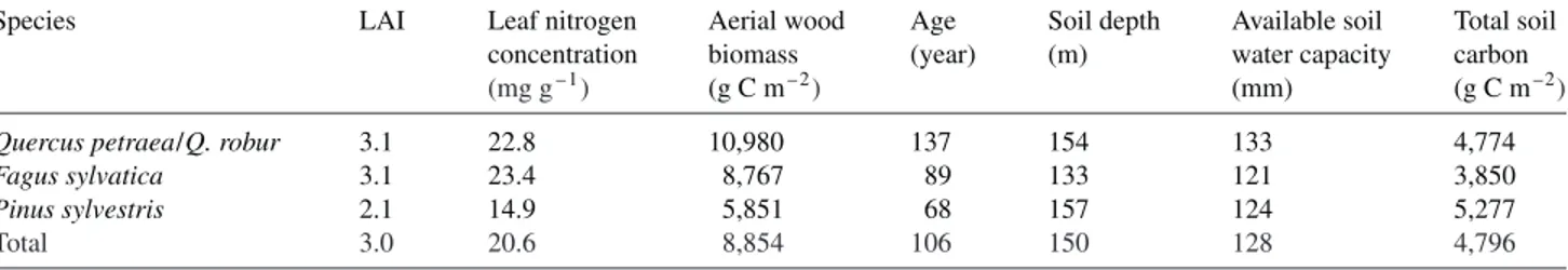
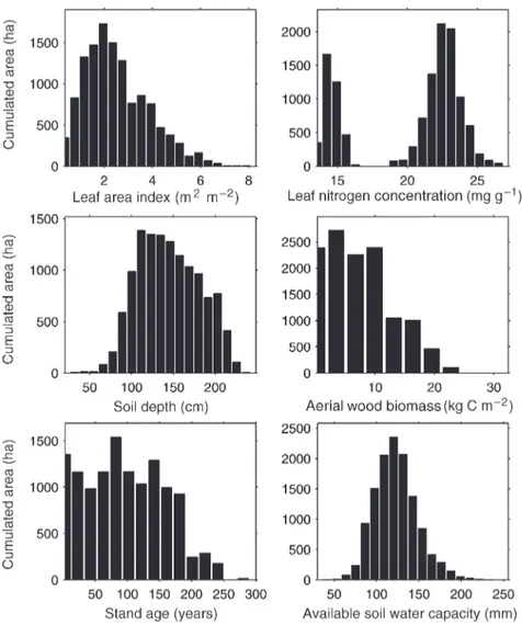
The model input parameters attributed to each stand are means and are reported as area-weighted for the three main tree spe-cies and for the entire forest (Table 3). The histograms pre-sented in Figure 5 represent the cumulated area of each parameter class. Stand LAI values range from less than 1 to 8. Low values represent seed tree stands or sparsely wooded ar-eas; high values are dense closed canopies. The leaf Nm histo-gram is bimodal: the low values represent coniferous stands, and the high values represent deciduous stands. The distribu-tion for coniferous stands is less spread out, showing that co-niferous stands are mainly on the same type of soil (brown podzol), whereas the deciduous stands are mainly on argilic brown soils. Soil depth varies widely in the Fontainebleau for-est, ranging from 100 to more than 200 cm. Aboveground wood biomass and age are typical for a managed forest com-prising many different-aged stands. Available soil water ca-pacity is low, mainly because of the sandy soils, but can reach values of 200 mm.
Simulation results
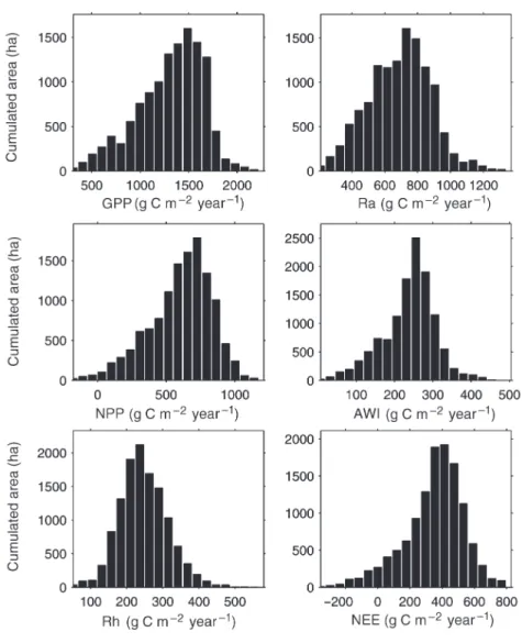
The simulation results are weighted by stand area and aver-aged over the whole forest as described in Equation 4 ( Ta-ble 4). Each output is expressed as g C m– 2year– 1. For the parameterization, results are given by species for the three main species of the forest, and in total for the whole forest. Histograms are also presented (Figure6). Annual GPP values range from low values (low LAI stands) to more than 2000 g C m– 2year– 1(Scots pines stands with high LAI). The annual NPP histogram shows some negative values, perhaps indicat-ing errors in parameterization as a result of errors in the data set; e.g., overestimation of wood biomass of the stand would lead to overestimation of autotrophic respiration. The NEE is mainly positive but some stands show negative values (i.e., carbon source).
Maps ofAWI and NEE are presented inFigure7. They illus-trate the high variability in stand functioning, creating a com-plex mosaic with apparently no spatial correlations. However, the species spatial distribution explains a part of the spatial dis-tribution in NEE and AWI (Figure 1).
Trunk wood volume of the forest is about 2.6 × 10⁶m3and the volume increment is 7.1 × 10⁴m3(2.74%) for the year 1995 (Table5). Estimates made by IFN and ONF are given for
Table 3. Mean values of key parameters scaled stand by stand over the Fontainebleau forest. Results are weighted by stand area and averaged by species, and calculated for the whole forest (Total).
Species LAI Leaf nitrogen Aerial wood Age Soil depth Available soil Total soil
concentration biomass (year) (m) water capacity carbon
(mg g– 1) (g C m– 2) (mm) (g C m– 2)
Quercus petraea/Q. robur 3.1 22.8 10,980 137 154 133 4,774
Fagus sylvatica 3.1 23.4 8,767 89 133 121 3,850 Pinus sylvestris 2.1 14.9 5,851 68 157 124 5,277 Total 3.0 20.6 8,854 106 150 128 4,796 Au: Please provide the ini-tials for Dhote and the institu-tional affilia-tion. Au: Where is Equation 4? And Equation 3?
comparison, either for the entire forest or for the principal spe-cies.
Discussion
Parameterization methodology
Unlikestatistical empirical models, the CASTANEA model is a process-based ecophysiological model that requires many input parameters. We were able to obtain most of these param-eters for the Fontainebleau forest. The CASTANEA model was created to simulate the carbon and water fluxes for
homo-geneous forest stands, and was validated on n homohomo-geneous stands with flux tower and growth data. However, the para-meterization of the model at this scale proved difficult, and an unknown source of error or bias may have been introduced.
The stands are consideredto be even-aged, homogeneous in species, structure, tree densityand spatial distribution of trees. This is the case for most of them (it was the polygon delinea-tion criterion). However, some stands may have an irregular structure, which may create bias in the results because of the non-linearity process. A similar bias may also occur when stand mean parameters values are used.
Figure 5. Histograms of the distribu-tion of input parameters. Thex-axis is the parameter class and the y-axis is the cumulated area for the considered class.
Table 4. Carbon flux (gC m– 2year– 1) outputs averaged on the Fontainebleau forest, species by species and on the whole forest.Abbreviations: GPP = gross primary productivity; NPP = net primary productivity; and NEE = net ecosystem exchange.
Species GPP Autotrophic NPP Aboveground woody Heterotrophic NEE
respiration biomass increment respiration
Quercus petraea/Q. robur 1408 –737 672 244 –263 409
Fagus sylvatica 1225 –693 532 252 –232 301
Pinus sylvestris 1357 –699 658 260 –268 390
Figure 6. Histograms of the distribu-tion of output fluxes(g C m– 2year– 1):
gross primary production (GPP), autotrophic respiration (Ra), net pri-mary productivity (NPP), aboveground wood increment (AWI), heterotrophic respiration (Rh) and net ecosystem ex-change (NEE). The x-axis is the pa-rameter class and the y-axis is the cumulated area for the considered class.
Weassumed no interaction among stands, i.e., each stand functions independently of the surrounding stands. This hy-pothesis is justified for the hydrology because: (1) the topogra-phy is flat in the wooded areas; and (2) because the soil is sandy and deep, so there is essentially no horizontal runoff. Another possible interaction is shadowing, especially if a tall stand is located south of a small stand, but this effect is likely to be small. Finally, an interaction could be more climatic, for example wind speed or relative humidity, but these effects are difficult to quantify and include in a model.
The climate was not spatialized. A fine grid of meteorologi-cal data was computed with the model AURHELY developed by Météo-France (Bénichou and Le Breton 1987). This model uses meteorological data from local stations and interpolates the data taking account of topography. A preliminary analysis of these interpolated data showed only small differences with the mean value in the areas of interest; therefore, the hypothe-sis of a mean climate over the forest seems justified, but needs further investigation.
Leaf area index was deduced from a relationship with the standard deviation of the NDVIs of the stand. The use of poly-gon-based aggregation of remotely sensed data for LAI esti-mation can provide more inforesti-mation than pixel-based estimations (Wicks et al. 2002). The NDVI standard deviation is a quantification of the heterogeneity inside the stand. In a managed forest, the LAI of a stand is closely linked to hetero-geneity: a small LAI implies open canopies, with large gaps (e.g., seed tree stands), leading to high heterogeneity, whereas a high LAI is obtained when the canopy is closed and more ho-mogeneous. A second explanation for the close correlation be-tween the NDVI standard deviation and ground-measured LAI is the saturation of the LAI–NDVI relationship: at low LAI, this relationship is quite linear, so for small changes in LAI from one pixel to another inside the stand, there is a propor-tional change in NDVI. But at high LAI, a small change in LAI only slightly affects the pixel NDVI value, as reflected in the higher NDVI standard deviation for low LAI distributions, and the smaller NDVI standard deviation for high LAI distribu-tions.
The relationship between soil type and leaf Nmcan be ex-plained on the basis of soil fertility. The Fontainebleau forest includes a wide range of soil types, allowing for a rough esti-mate of leaf Nm. Work is being done to develop a more precise
estimate of Nmbased on hyperspectral satellite images (Diker and Bausch 2003, Graeff and Claupein 2003, Hansen and Schjoerring 2003). An advantage of the relationship we used is that soil fertility is accounted for in the simulations through leaf Nm, which is directly linked to leaf photosynthetic capa-city. Stands located on poor soils (e.g., brown podzol) will have lower leaf Nm, leading to lower photosynthesis and growth compared with stands on fertile soils.
The soil equilibrium hypothesis assumes that soil carbon in-puts (litter fall and root fall)approximate carbon outputs from heterotrophic respiration. The difference between these two fluxes depends on annual climate variations. This hypothesis has previously been tested for soil respiration efflux and gives good agreement for deciduous species (Epron et al. 2001, Yang et al. 2002). For coniferous species, we think that the simulated fluxes are overestimated: under a coniferous can-opy, there is generally an accumulation of carbon (King 1995), which is in contradiction with the equilibrium hypothesis.
Simulation of carbon fluxes over a large forest requires great simplifications: many parameters are extremely respon-sive in the model and highly spatially variable (e.g., LMA), but are not easily measured at this scale. The spatialization of LMA could be done through remote sensing, but no such LMA data for a forest canopy are currently available (Blackburn and Steele 1999).
We did not consider the effects of the mixing of species in-side a stand, either involving the three main species (oak, beech and pine), or including codominant species (hornbeam or birch). In our simulations, the species attribution for each stand is the main species of the stand. For deciduous mixed species, the effect on stand flux should be low because we esti-mated LAI based on the total leaf area of the stand. The basal area is also the total of the stand. Therefore the small variation caused by the slightly differing functioning of oak and beech would be simulated. For mixed coniferous–deciduous species, use of the mean parameters of the dominant species is inade-quate because phenology, photosynthesis and respiratory pro-cesses differ greatly among species. However, because the stands of mixed coniferous–deciduous species represent less than 10% of the forest, if the criterion for heterogeneity is that the dominant species represents less than 80% of the canopy cover of the stand, we suppose that the errors thus made would be negligible. Finally, the understory coverage can have a large Table 5. Wood volume estimate of the Fontainebleau forest for the year 1995 obtained by the National Forest Inventory (IFN) and by the French National Forest Office (ONF). The volume increment of the year 1995 was estimated by the IFN. Relative growth ratio (RGR) is the ratio of the volume increment divided by the volume. Results are presented by species and for the whole Fontainebleau forest.
Species IFN volume ONF volume Volume IFN volume Volume IFN RGR Estimated RGR
(m3) (m3) estimated increment increment (% vol. year– 1) (% vol. year– 1)
(m3) (m3year– 1) (m3year– 1)
Quercus petraea/Q. robur 1,297,281 1,076,303 1,344,000 23,923 28,000 1.84 2.08
Fagus sylvatica 414,390 333,589 325,520 14,254 8,940 3.44 2.75
Pinus sylvestris 732,796 655,267 637,150 21,989 25,123 3.00 3.94
Other species 266,057 227,527 295,400 8,008 9,106 3.01 3.08
effect on stand water fluxes. The understory can reach an LAI that will greatly influence the water content of the top soil, and thereby modify stand carbon fluxes directly (understory GPP and Ra) or indirectly through soil water status. It is difficult to account for the understory because we have little knowledge of its function in terms of carbon and water fluxes and it is dif-ficult to map it over the whole forest.
The rocky areas, representing about 15% of the total forest surface, were not simulated. These areas, with superficial soils,are sparsely wooded, mostly boulder covered and slop-ing. Their wood production and carbon fluxes were considered to be negligible compared with the rest of the forest. For the forest area with species for which the CASTANEA model was not parameterized, which represent only about 5% of the forest area, the carbon fluxes were simulated with parameters from ecologically comparable species. Comparison with the ONF and IFN estimates of wood volume and annual volume in-crease was realized separately for the three dominant species.
Simulations
For deciduous species, Fluxnet towers measurements of GPP were between 1100 and 1700 g C m– 2year– 1and between 700 and 2200 g C m– 2year– 1for coniferous species, depending on location, year and stand age. For deciduous stands in a temper-ate climtemper-ate, GPP measurements range from 950 to 1700 g C m– 2year– 1(4 sites: Hesse, France; Harvard Forest, MA, USA; Walker Branch, TN, USA; Willow Creek, WI, USA). For co-niferous stands in a temperate climate, GPP measurements range between 1100 and 1500 g C m– 2year– 1(3 sites: Duke, NC, USA; Loobos, Netherlands; and Metolius, OR, USA) (Law et al. 2002, Valentini et al. 2000). Thus, our GPP simula-tions fall within the range of measured GPP values.
Measurements of NEEat these same Fluxnet sites ranged from –50 to 870 g C m– 2 year– 1for deciduous species and from 260 to 650 g C m– 2year– 1for coniferous species. The values obtained in our simulations fall into these ranges for de-ciduous and evergreen stands on average, and for most of the stands separately (Figures 6 and 7).
Our simulated heterotrophic respiration rates are ques-tionable, especially the finding that respiration in coniferous stands is of the same order of magnitude as in deciduous stands. The simulations may indicate that the approach used to initialize the carbon pools is inadequate or that there is little lit-ter accumulation (equilibrium hypothesis). This result directly affects simulated NEE.
Our simulated NPP in Fontainebleau (630 g C m– 2year– 1) is only slightly higher than the MODIS value of 590 g C m– 2 year– 1 derived from large-scale satellite based calculations (Turner et al. 2003). We compared our results with measure-ments made by both IFN and ONF for the whole Fontaine-bleau forest (Table 5). Our calculation of volume is in agreement with the IFN estimates for the whole forest, with a 4% difference in the total; however, there is a 14% difference with the ONF volume estimates.
Simulated volume increment is also in good agreement with the IFN estimation (5% difference in total). Trunk relative
growth ratio (RGR, volume increment divided by the volume and expressed as a percentage increment per year) provides a way to compare our forest productivity estimates with those of the IFN. Our RGR values are in good agreement with the IFN values for the Quercus species, slightly lower for Fagus and overestimated for Pinus. In total, we overestimated forest pro-ductivity by 9%.
Possible reasons for these discrepancies are: (1) the year 1995 had favorable climatic conditions, with more precipita-tion than normal, limiting the autumn drought, so NPP was about 10% higher than the mean over 30 years of climatic data; (2) the conversion from daily to half-hourly climatic data leads to an overestimation of NPP of about 10%, because days with high radiation variability were not simulated in the half-hourly transformed data; and (3) the possible presence of nutrient limitation, especially phosphorus (P), which is not accounted for in the model. Mean leaf phosphorus concentration in the Fontainebleau forest is around 1 mg g– 1for beeches and oaks and 0.9 mg g– 1for Scots pines. For comparison, mean P values of various forests in France are generally 1.35 mg g– 1for oaks, 1.24 mg g– 1 for beeches and 1.33 mg g– 1 for Scots pines (Croisé et al. 1999). Phosphorus limitation can affect forest productivity (Bauer et al. 1997, Loustau et al. 1999, Warren and Adams 2002).
The model may overestimate or underestimate aboveground wood incrementbecause of the simplicity of the carbon alloca-tion module. This module ignores possible variaalloca-tions between stands differing in age and fertility. In aged and nutrient-poor stands, carbon allocation to fine roots could be enhanced (Magnani et al. 2000) and therefore greater than the constant value used in the model. Moreover, the older the stand, the greater its biomass and simulated autotrophic respiration, which leads to a greater use of carbohydrate storage during the winter. So, allocation to reserves, which was calibrated for young stands, could be underestimated for the oldest stands. If these two carbon sinks were underestimated for part of the for-est, we probably overestimated the aboveground wood incre-ment. Nevertheless, a bias in the carbon balance between aboveground and underground compartments will have little effect on the NPP and NEE estimates because fine roots and aboveground wood have similar construction and maintenance costs.
Conclusion
We attempted to estimate carbon fluxes of a whole forest. Our results underline the importance of precise parameterization and validation. Our approach, consisting of stand-by-stand simulations, with attributes derived from forest inventories, soil inventories, satellite data and field measurements, shows good potential. More field measurements are needed to spa-tially validate our results. Soil respiration measurements are now in progress, as well as growth estimates from stem cores. We used an ancillary growth data set to improve the accuracy of the carbon allocation model, particularly to reproduce the decline in NPP with stand age more accurately (Gower et al.
1996). Our productivity results differ slightly from, but are close to, the growth estimates of the IFN. Reasonably good agreement was found between simulated trunk RGR (2.74%) and regional production estimates by the IFN (2.52%), as well as between simulated amd measured annual wood production at the forest scale (around 71,000 m3year– 1and 68,000 m3 year– 1, respectively). This work contributes to the effort to model climate change effects on forest productivity at the re-gional scale.
Acknowledgments
The authors thank the French National Forest Office (ONF) for provision of the database and for letting us study the experimental stands in the Fontainebleau forest. This research was supported by the GIP EcoFor and the Observatoire de Recherche en Environnement (ORE, French Ministry of Ecology).
References
Baize, D. 1988. Guide des analyses courantes en pédologie. INRA, Paris, 172 p.
Baldocchi, D.D. and P.C. Harley. 1995. Scaling carbon-dioxide and water vapor exchange from leaf to canopy in a deciduous forest. 2. Model testing and application. Plant Cell Environ. 18:1157–1173. Ball, J.T., I.E. Woodrow and J.A. Berry. 1987. A model predicting
stomatal conductance and its contribution to the control of pho-tosynthetis under different environmental conditions. In Progress in Photosynthesis Research. Ed. J. Biggens. Martinus Nijhoff, Dordrecht, pp 221–224.
Barbaroux, C. 2002. Analyse et modélisation des flux de carbone de peuplements forestiers pour la compréhension de la croissance des espèces feuillues Quercus petraea et Fagus sylvatica. Université Paris XI, Orsay, 183 p.
Barbaroux, C., N. Bréda and E. Dufrêne. 2003. Distribution of above-ground and below-ground carbohydrate reserves in adult trees of two contrasting broad-leaved species (Quercus petraea and
Fagus sylvatica). New Phytol. 157:605–615.
Bauer, G., E.-D. Schulze and M. Mund. 1997. Nutrient contents and concentrations in relation to growth of Picea abies and Fagus
sylvatica along a European transect. Tree Physiol. 17:777–786.
Bauhus, J. and N. Bartsch. 1996. Fine-root growth in beech (Fagus
sylvatica) forest gaps. Can. J. For. Res. 26:2153–2159.
Bénichou, P. and O. Le Breton. 1987. Prise en compte de la topo-graphie pour la cartotopo-graphie des champs pluviométriques sta-tistiques. La Météorologie. 7:23–34.
Berbigier, P., J.-M. Bonnefond and P. Mellmann. 2001. CO2and water vapour fluxes for 2 years above Euroflux forest site. Agric. For. Meteorol. 108:183–197.
Blackburn, G.A. and C.M. Steele. 1999. Towards the remote sensing of matorral vegetation physiology; relationships between spectral reflectance, pigment and biophysical characteristics of semiarid bushland canopies. Remote Sens. Environ. 70:278–292. Brêthes, A. and E. Ulrich. 1997. RENECOFOR—Caractéristiques
pédologiques des 102 peuplements du réseau. Office National des Forêts, 573 p.
Cairns, M.A., S. Brown, E.H. Helmer and G.A. Baumgardner. 1997. Root biomass allocation in the world’s upland forests. Oecologia 111:1–11.
Ceschia, E., C. Damesin, S. Lebaube, J.-Y. Pontailler and E. Dufrêne. 2002. Spatial and seasonal variations in stem respiration of beech trees (Fagus sylvatica). Ann. For. Sci. 59:801–812.
Croisé, L., C. Cluzeau, E. Ulrich, M. Lanier and A. Gomez. 1999. RENECOFOR—interprétation des analyses foliaires réalisées dans les 102 peuplements du réseau de 1993 à 1997 et premières évaluations interdisciplinaires. Office National des Forêts, Département recherche et Développement, 413 p.
Damesin, C., E. Ceschia, N. Le Goff, J.M. Ottorini and E. Dufrêne. 2002. Stem and branch respiration of beech: from tree measure-ments to estimations at the stand level. New Phytol. 153:159–172. Davi, H. 2004. Développement d’un modèle forestier générique
simulant les flux et les stocks de carbone et d’eau dans le cadre des changements climatiques. Université Paris XI, Orsay, 194 p. Demarez, V., J.P. Gastellu-Etchegorry, E. Mougin, G. Marty,
C. Proisy, E. Dufrene and V. Le Dantec. 1999. Seasonal variation of leaf chlorophyll content of a temperate forest. Inversion of the PROSPECT model. Int. J. Remote Sens. 20:879–894.
Dhote, J.F. 1991. Modeling the growth of even-aged beech stands—dynamics of hierarchical systems and yield factors. Ann. For. Sci. 48:389–416.
Diker, K. and W.C. Bausch. 2003. Potential use of nitrogen reflectance index to estimate plant parameters and yield of maize. Biosyst. Eng. 85:437– 447.
Ditzer, T., R. Glauner, M. Förster, P. Köhler and A. Huth. 2000. The process-based stand growth model Formix 3-Q applied in a Gis en-vironment for growth and yield analysis in a tropical rain forest. Tree Physiol. 20:367–381.
Dolman, A.J., E.J. Moors and J.A. Elbers 2002. The carbon uptake of a mid-latitude pine forest growing on sandy soil. Agric. For. Meteorol. 111:157–170.
Duchaufour, P. 1982. Pedology. George Allen and Unwin, London, 448 p.
Dufrêne, E., V. Le Dantec, V. Demarez, J.P. Gastellu-Etchegorry, G. Marty, E. Mougin, C. Proisy, B. Lacaze and S. Rambal. 1997. Remote sensing of the Fontainebleau forest during EMAC-94: ob-jectives and data collection program. In EMAC 94/95, Final Re-sults. ESASP, ESTEC, Noordwijk, NL, pp 91–95.
Epron, D., V. Le Dantec, E. Dufrêne and A. Granier. 2001. Seasonal dynamics of soil carbon dioxide efflux and simulated rhizosphere respiration in a beech forest. Tree Physiol. 21:145–152.
Farquhar, G.D., S. von Caemmerer and J.A. Berry. 1980. A biochemi-cal model of photosynthetic CO2assimilation in leaves of C3 spe-cies. Planta 149:78 – 80.
François, C. 2002. The potential of directional radiometric tempera-tures for monitoring soil and leaf temperature and soil moisture sta-tus. Remote Sens. Environ. 80:122–133.
Gower, S.T., S. Pongracic and J.J. Landsberg. 1996. A global trend in belowground carbon allocation: can we use the relationship at smaller scales? Ecology 77:1750–1755.
Graeff, S. and W. Claupein. 2003. Quantifying nitrogen status of corn (Zea mays L.) in the field by reflectance measurements. Eur. J. Agron. 19:611–618.
Granier, A., E. Ceschia, C. Damesin et al. 2000. The carbon balance of a young beech forest. Funct. Ecol. 14:312–325.
Hansen, P.M. and J.K. Schjoerring. 2003. Reflectance measurement of canopy biomass and nitrogen status in wheat crops using nor-malized difference vegetation indices and partial least squares re-gression. Remote Sens. Environ. 86:542–553.
Hatsch, E. 1997. Répartition de l’aubier et acquisition de la forme de la tige chez le chêne sessile: analyse, modélisation et relation avec le développement du houppier. ENGREF, Paris, 183 p.
He, H.S., D.J. Mladenoff and T.R. Crow. 1999. Linking an ecosystem model and a landscape model to study forest species response to climate warming. Ecol. Model. 114:213–233.
Au: Please provide the city and country of the publish-er for Brêthes and Ulrich 1997 and for
Hoffmann, F. 1995. FAGUS, a model for growth and development of beech. Ecol. Model. 83:327–348.
King, D.A. 1995. Equilibrium analysis of a decomposition and yield model applied to Pinus radiata plantations on sites of contrasting fertility. Ecol. Model. 83:349–358.
Kirschbaum, M.U.F. 1999. CenW, a forest growth model with linked carbon, energy, nutrient and water cycles. Ecol. Model. 118:17–59. Kramer, K., I. Leinonen, H.H. Bartelink et al. 2002. Evaluation of six process-based forest growth models using eddy-covariance mea-surements of CO2and H2O fluxes at six forest sites in Europe. Global Change Biol. 8:213–230.
Landsberg, J. 2003. Modelling forest ecosystems: state of the art, challenges and future directions. Can. J. For. Res. 33:385–397. Law, B.E., E. Falge, L. Gu et al. 2002. Environmental controls over
carbon dioxide and water vapor exchange of terrestrial vegetation. Agric. For. Meteorol. 113:97–120.
Le Dantec, V. 2000. Modélisation des échanges carbonés et hydriques dans un écosystème forestier: un modèle couplé sol–plante. Université Paris XI, Orsay.
Le Dantec, V., E. Dufrêne and B. Saugier. 2000. Interannual and spa-tial variation in maximum leaf area index of temperate deciduous stands. For. Ecol. Manage. 134:71–81.
Lehtonen, A., R. Makipaa, J. Heikkinen, R. Sievanen and J. Liski. 2004. Biomass expansion factors (BEFs) for Scots pine, Norway spruce and birch according to stand age for boreal forests. For. Ecol. Manage. 188:211–224.
Loustau, D., M. Ben Brahim, J.P. Gaudillère and E. Dreyer. 1999. Photosynthetic responses to phosphorus nutrition in two-year-old maritime pine seedlings. Tree Physiol. 19:707–715.
Magnani, F., M. Mencuccini and J. Grace. 2000. Age-related decline in stand productivity: the role of structural acclimation under hy-draulic constraints. Plant Cell Environ. 23:251–263.
Mäkelä, A., J. Landsberg, A.R. Ek, T.E. Burk, M. Ter-Mikaelian, G.I. Agren, C.D. Oliver and P. Puttonen. 2000. Process-based models for forest ecosystem management: current state of the art and chal-lenges for practical implementation. Tree Physiol. 20:289–298. Monteith, J.L. 1965. Evaporation and environment. Symp. Soc. Exp.
Biol. 19:205–233.
Myneni, R.B., J. Dong, C.J. Tucker, R.K. Kaufmann, P.E. Kauppi, J. Liski, L. Zhou, V. Alexeyev and M.K. Hughes. 2001. A large car-bon sink in the woody biomass of northern forests. PNAS 98: 14,784 –14,789.
Parton, W.J., D.S. Schimel, C.V. Cole and D.S. Ojima. 1987. Analysis of factors controlling soil organic matter levels in Great Plains grasslands. Soil Sci. Soc. Am. J. 51:1173–1179.
Penman, H.L. 1948. Natural evaporation from open water, bare soil and grass. Proc. R. Soc. Lond. 193:120–145.
Penning de Vries, F.W.T. 1975. The cost of maintenance processes in plant cells. Ann. Bot. 39:77–92.
Penning de Vries, F.W.T., A.H.M. Brunsting and H.H. Van Laar. 1974. Products, requirement and efficiency of biosynthesis: a quantitative approach. J. Theor. Biol. 45:339–377.
Plummer, S.E. 2000. Perspectives on combining ecological process models and remotely sensed data. Ecol. Model. 129:169–186. Proisy, C., E. Mougin, E. Dufrêne and V. Le Dantec. 2000.
Monitor-ing seasonal changes of a mixed temperate forest usMonitor-ing ERS SAR observations. IEEE Trans. Geosci. Remote Sens. 38:540–552. Robin, A.-M. 1993. Catalogue des principales stations forestières de
la forêt de Fontainebleau. Office National des Forêts/Université Pierre et Marie Curie, 371 p.
Running, S.W., D.D. Baldocchi, D.P. Turner, S.T. Gower, P.S. Bakwin and K.A. Hibbard. 1999. A global terrestrial monitoring network integrating tower fluxes, flask sampling, ecosystem mod-eling and EOS satellite data. Remote Sens. Environ. 70:108–127. Rutter, A.J., K.A. Kershaw, P.C. Robins and A.J. Morton. 1971. A
predictive model of rainfall interception in forests. I. Derivation of the model from observations in a plantation of Corsican pine. Agric. For. Meteorol. 9:367–384.
Ryan, G.M. 1991. Effects of climate change on plant respiration. Ecol. Appl. 1:157–167.
Sala, A. and J.D. Tenhunen. 1996. Simulations of canopy net photo-synthesis and transpiration in Quercus ilex L. under the influence of seasonal drought. Agric. For. Meteorol. 78:203–222.
Santantonio, D. 1989. Dry-matter partitioning and fine-root pro-duction in forests: new approaches to a difficult problem. In Bio-mass Production by Fast-Growing Trees. Eds. J.S. Pereira and J.J. Landsberg. Kluwer Academic Publishers, Dordrecht, pp 57–72.
Saxton, K.E., W.J. Rawls, J.S. Romberger and R.I. Papendick. 1986. Estimating generalized soil-water characteristics from texture. Soil Sci. Soc. Am. J. 50:1031–1036.
Schober, R. 1975. Ertragstafeln wichtiger Baumgarten bei verschie-denen Durchforstung. J.D. Sauerländer’s Verlag, Frankfurt am Main, 154 p.
Song, C., C.E. Woodcock, K.C. Seto, M.P. Lenney and S.A. Ma-comber. 2001. Classification and change detection using Landsat TM data: when and how to correct atmospheric effects? Remote Sens. Environ. 75:230–244.
Stenberg, P., S. Linder, H. Smolander and J. Flower-Ellis. 1994. Per-formance of the LAI-2000 plant canopy analyzer in estimating leaf area index of some Scots pine stands. Tree Physiol. 14:981–995. Turner, D.P., W.D. Ritts, W.B. Cohen et al. 2003. Scaling gross
pri-mary production (GPP) over boreal and deciduous forest land-scapes in support of MODIS GPP product validation. Remote Sens. Environ. 88:256–270.
Valentini, R., G. Matteucci, A.J. Dolman et al. 2000. Respiration as the main determinant of carbon balance in European forests. Nature 404:861–865.
Verhoef, W. 1984. Light scattering by leaf layers with application to canopy reflectance modeling: the SAIL model. Remote Sens. Envi-ron. 16:125–141.
Verhoef, W. 1985. Earth observation modeling based on layer scatter-ing matrices. Remote Sens. Environ. 17:165–178.
Vogt, K.A., D.J. Vogt, E.E. Moore, B.A. Fatuga, M.R. Redlin and R.L. Edmonds. 1987. Conifer and angiosperm fine-root biomass in relation to stand age and site productivity in Douglas-fir forests. J. Ecol. 75:857–870.
Warren, C.R. and M.A. Adams. 2002. Phosphorus affects growth and partitioning of nitrogen to Rubisco in Pinus pinaster. Tree Physiol. 22:11–19.
Wicks, T.E., G.M. Smith and P.J. Curran. 2002. Polygon-based aggre-gation of remotely sensed data for regional ecological analyses. Int. J. Applied Earth Observation and Geoinformation 4:161–173. Wullschleger, S.D. 1993. Biochemical limitations to carbon
assimila-tion in C3plants—a retrospective analysis of the A/Cicurves from 109 species. J. Exp. Bot. 44:907–920.
Yang, X., M. Wang, Y. Huang and Y. Wang. 2002. A one-compart-ment model to study soil carbon decomposition rate at equilibrium situation. Ecol. Model. 151:63–73.
Au: Please provide the total no. of pages for Le Dantec 2000. Au: Please provide the loca-tion of the pub-lisher for Robin 1993.