HAL Id: hal-01102028
https://hal.archives-ouvertes.fr/hal-01102028
Submitted on 11 Jan 2015
HAL is a multi-disciplinary open access
archive for the deposit and dissemination of
sci-entific research documents, whether they are
pub-lished or not. The documents may come from
teaching and research institutions in France or
abroad, or from public or private research centers.
L’archive ouverte pluridisciplinaire HAL, est
destinée au dépôt et à la diffusion de documents
scientifiques de niveau recherche, publiés ou non,
émanant des établissements d’enseignement et de
recherche français ou étrangers, des laboratoires
publics ou privés.
Wiem Maalel, Kuang Zhou, Arnaud Martin, Zied Elouedi
To cite this version:
Wiem Maalel, Kuang Zhou, Arnaud Martin, Zied Elouedi. Belief Hierarchical Clustering. 3rd
Interna-tional Conference on Belief Functions, Sep 2014, Oxford, United Kingdom. pp.68 - 76,
�10.1007/978-3-319-11191-9_8�. �hal-01102028�
Belief Hierarchical Clustering
Wiem Maalel, Kuang Zhou, Arnaud Martin, and Zied Elouedi LARODEC, ISG.41 rue de la Libert´e, 2000 Le Bardo, Tunisia
IRISA, Universit´e de Rennes 1. IUT de Lannion. Rue Edouard Branly BP 30219, 22302 Lannion cedex. France
[email protected] [email protected] [email protected]
Abstract. In the data mining field many clustering methods have been proposed, yet standard versions do not take into account uncertain databases. This paper deals with a new approach to cluster uncertain data by using a hierarchical clustering defined within the belief function framework. The main objective of the belief hierarchical clustering is to allow an object to belong to one or several clusters. To each belonging, a degree of belief is associated, and clusters are combined based on the pignistic properties. Experiments with real uncertain data show that our proposed method can be considered as a propitious tool.
Keywords: Clustering, Hierarchical clustering, Belief function, Belief clustering
1
Introduction
Due to the increase of imperfect data, the process of decision making is becoming harder. In order to face this, the data analysis is being applied in various fields. Clustering is mostly used in data mining and aims at grouping a set of similar objects into clusters. In this context, many clustering algorithms exist and are categorized into two main families:
The first family involves the partitioning methods based on density such as k-means algorithm [6] that is widely used thanks to its convergence speed. It par-titions the data into k clusters represented by their centers. The second family includes the hierarchical clustering methods such as the top-down and the Hi-erarchical Ascendant Clustering (HAC) [5]. This latter consists on constructing clusters recursively by partitioning the objects in a bottom-up way. This process leads to good result visualizations. Nevertheless, it has a non-linear complexity. All these standard methods deal with certain and precise data. Thus, in order to facilitate the decision making, it would be more appropriate to handle uncertain data. Here, we need a soft clustering process that will take into account the possibility that objects belong to more than one cluster.
In such a case, several methods have been established. Among them, the Fuzzy C-Means [1] which consists in assigning a membership to each data point
corresponding to the cluster center, and the weights minimizing the total weighted mean-square error. This method constantly converges. Patently, Evidential c-Means (ECM) [3], [7] is deemed to be a very fateful method. It enhances the FCM and generates a credal partition from attribute data. This method deals with the clustering of object data. Accordingly, the belief k-Modes method [4] is a popular method, which builds K groups characterized by uncertain attribute values and provides a classification of new instances. Schubert has also found a clustering algorithm [8] which uses the mass on the empty set to build a classifier. Our objective in this paper is to develop a belief hierarchical clustering method, in order to ensure the membership of objects in several clusters, and to handle the uncertainty in data under the belief function framework.
This remainder is organized as follows: in the next section we review the ascendant hierarchical clustering, its concepts and its characteristics. In section 3, we recall some of the basic concepts of belief function theory. Our method is described in section 4 and we evaluate its performance on a real data set in section 5. Finally, Section 6 is a conclusion for the whole paper.
2
Ascendant hierarchical clustering
This method consists on agglomerating the close clusters in order to have finally one cluster containing all the objects xj (where j = 1, .., N ).
Let’s consider PK= {C
1, ..., CK} the set of clusters. If K = N , C1= x1, ..., CN =
xN. Thereafter, throughout all the steps of clustering, we will move from a
par-tition PK to a partition PK−1. The result generated is described by a
hierar-chical clustering tree (dendrogram), where the nodes represent the successive fusions and the height of the nodes represents the value of the distance between two objects which gives a concrete meaning to the level of nodes conscripted as ”indexed hierarchy”. This latter is usually indexed by the values of the dis-tances (or dissimilarity) for each aggregation step. The indexed hierarchy can be seen as a set with an ultrametric distance d which satisfies these properties: i) x = y ⇐⇒ d(x, y) = 0.
ii) d(x, y) = d(y, x).
iii) d(x, y) ≤ d(x, z) + d(y, z), ∀x, y, z ∈ IR. The algorithm is as follows:
– Initialisation: the initial clusters are the N-singletons. We compute their dissimilarity matrix.
– Iterate these two steps until the aggregation turns into a single cluster: • Combine the two most similar (closest) elements (clusters) from the
se-lected groups according to some distance rules.
• Update the matrix distance by replacing the two grouped elements by the new one and calculate its distance from each of the other classes. Once all these steps completed, we do not recover a partition of K clusters, but a partition of K − 1 clusters. Hence, we had to point out the aggregation
Belief Hierarchical Clustering 3
criterion (distance rules) between two points and between two clusters. We can use the Euclidian distance between N objects x defined in a space IR. Different distances can be considered between two clusters: we can consider the minimum as follows:
d(Cji, Cji′) = min
xk∈Cji,xk′∈Cj′i
d(xk, xk′) (1)
with j, j′= 1, ..., i. The maximum can also be considered, however, the minimum
and maximum distances create compact clusters but sensitive to ”outliers”. The average can also be used, but the most used method is Ward’s method, using Huygens formula to compute this:
∆Iinter(Ci j,Cj′i)= mCjmCj′ mCj+ mCj′ d2(Cij, C i j′) (2)
where mCj and mCj′ are numbers of elements of Cj and Cj′ respectively and
Ci j, C
i
j′ the centers. Then, we had to find the couple of clusters minimizing the
distance: (Ck l, Clk′) = d(Cli, Cli′) = min Ci j,Cil′∈C i d(Ci j, Cji′) (3)
3
Basis on the theory of belief functions
In this Section, we briefly review the main concepts that will be used in our method that underlies the theory of belief functions [9] as interpreted in the Transferable Belief Model (TBM) [10]. Let’s suppose that the frame of discern-ment is Ω = {ω1, ω2, ..., ω3}. Ω is a finite set that reflects a state of partial
knowledge that can be represented by a basis belief assignment defined as: m: 2Ω → [0, 1]
P
A⊆Ω
m(A) = 1 (4)
The value m(A) is named a basic belief mass (bbm) of A. The subset A ∈ 2Ω is
called focal element if m(A) > 0. One of the important rules in the belief theory is the conjunctive rule which consists on combining two basic belief assignments m1 and m2 induced from two distinct and reliable information sources defined
as:
m1 ∩ m2(C) =
X
A∩B=C
m1(A) · m2(B), ∀C ⊆ Ω (5)
The Dempster rule is the normalized conjunctive rule: m1⊕ m2(C) =
m1 ∩ m2(C)
1 − m1 ∩ m2(∅)
, ∀C ⊆ Ω (6) In order to ensure the decision making, beliefs are transformed into proba-bility measures recorded BetP, and defined as follows [10]:
BetP(A) = X B⊆Ω |A ∩ B | | B | m(B) (1 − m(∅)),∀A ∈ Ω (7)
4
Belief hierarchical clustering
In order to set down a way to develop a belief hierarchical clustering, we choose to work on different levels: on one hand, the object level, on the other hand, the cluster level. At the beginning, for N objects we have, the frame of discernment is Ω= {x1, ..., xN} and for each object belonging to one cluster, a degree of belief
is assigned. Let PN be the partition of N objects. Hence, we define a mass
function for each object xi, inspired from the k-nearest neighbors [2] method
which is defined as follows: mΩi i (xj) = αe−γd 2(x i,xj) mΩi i (Ωi) = 1 −PmΩi i(xj) (8)
where i 6= j, α and γ are two parameters we can optimize [11], d can be con-sidered as the Euclidean distance, and the frame of discernment is given by Ωi= {x1, ..., xN} \ {xi}.
In order to move from the partition of N objects to a partition of N − 1 objects we have to find both nearest objects (xi, xj) to form a cluster.
Even-tually, the partition of N − 1 clusters will be given by PN −1 = {(x
i, xj), xk}
where k = 1, ..., N \ {i, j}. The nearest objects are found considering the pignis-tic probability, defined on the frame Ωi, of each object xi, where we proceed the
comparison by pairs, by computing firstly the pignistic for each object, and then we continue the process using arg max. The nearest objects are chosen using the maximum of the pignistic values between pairs of objects, and we will compute the product pair one by one.
(xi, xj) = arg max xi,xj∈PN BetPΩi i (xj) ∗ BetP Ωj j (xi) (9)
Then, this first couple of objects is a cluster. Now consider that we have a partition PK of K clusters {C
1, . . . , CK}. In order to find the best partition
PK−1of K − 1 clusters, we have to find the best couple of clusters to be merged.
First, if we consider one of the classical distances d (single link, complete link, average, etc), presented in section 2, between the clusters, we delineate a mass function, defined within the frame Ωi for each cluster Ci ∈ PK with Ci 6= Cj
by: mΩi i (Cj) = αe−γd 2(Ci,Cj) (10) mΩi i (Ωi) = 1 − X mΩi i (Cj) (11)
where Ωi= {C1, . . . , CK} \ {Ci}. Then, both clusters to merge are given by:
(Ci, Cj) = arg max Ci,Cj∈PK
BetPΩi(C
j) ∗ BetPΩj(Ci) (12)
and the partition PK−1is made from the new cluster (C
i, Cj) and all the other
Belief Hierarchical Clustering 5
degree of probability we will have the couple of clusters to combine. Of course, this approach will give exactly the same partitions than the classical ascendant hierarchical clustering, but the dendrogram can be built from BetP and the best partition (i.e. the number of clusters) can be preferred to find. The indexed hierarchy will be indexed by the sum of BetP which will lead to more precise and specific results according to the dissimilarity between objects and therefore will facilitate our process.
Hereafter, we define another way to build the partition PK−1. For each initial object xi to classify, it exists a cluster of PK such as xi ∈ Ck. We consider the
frame of discernment Ωi= {C1, . . . , CK} \ {Ck}, m, which describes the degree
that the two clusters could be merged, can be noted mΩand we define the mass
function: mΩi i (Ckj) = Y xj∈Ckj αe−γd2(xi,xj) (13) mΩi i (Ωi) = 1 − X xj∈Ckj mΩi i (Ckj) (14)
In order to find a mass function for each cluster Ci of PK, we combine all
the mass functions given by all objects of Ci by a combination rule such as
the Dempster rule of combination given by equation (6). Then, to merge both clusters we use the equation (12) as before. The sum of the pignisitic probabilities will be the index of the dendrogram, called BetP index.
5
Experimentations
Experiments were first applied on diamond data set composed of twelve objects as describe in Figure 1.a and analyzed in [7]. The dendrograms for both classical and Belief Hierarchical Clustering (BHC) are represented by Figures 1.b and 1.c. The object 12 is well considered as an outlier with both approaches. With the belief hierarchical clustering, this object is clearly different, thanks to the pig-nistic probability. For HAC, the distance between object 12 and other objects is small, however, for BHC, there is a big gap between object 12 and others. This points out that our method is better for detecting outliers. If the objects 5 and 6 are associated to 1, 2, 3 and 4 with the classical hierarchical clustering, with BHC these points are more identified as different. This synthetic data set is special because of the equidistance of the points and there is no uncertainty.
a. Diamond data set
b. Hierarchical clustering c. Belief hierarchical clustering
Fig. 1.Clustering results for Diamond data set.
We continue our experiments with a well-known data set, Iris data set, which is composed of flowers from four types of species of Iris described by sepal length, sepal width, petal length, and petal width. The data set contains three clusters known to have a significant overlap.
In order to reduce the complexity and present distinctly the dendrogram, we first used the k-means method to get initial few clusters for our algorithm. It is not necessary to apply this method if the number of objects is not high.
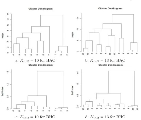
Several experiments have been used with several number of clusters. We present in Figure 2 the obtained dendrograms for 10 and 13 clusters. We notice different combinations between the nearest clusters for both classical and belief hierarchical clustering. The best situation for BHC is obtained with the pignistic equal to 0.5 because it indicates that the data set is composed of three significant clusters which reflects the real situation. For the classical hierarchical clustering
Belief Hierarchical Clustering 7
a. Kinit= 10 for HAC b. Kinit= 13 for HAC
c. Kinit= 10 for BHC d. Kinit= 13 for BHC
Fig. 2.Clustering results on IRIS data set for both hierarchical (HAC) (Fig. a and b) and belief hierarchical (BHC) (Fig. c and d) clustering (Kinitis the cluster number by
k-means first).
the results are not so obvious. Indeed, for HAC, it is difficult to decide for the optimum cluster number because of the use of the euclidean distance and as seen in Figure 2.c it indistinguishable in terms of the y-value. However, for BHC, it is more easy to do this due to the use of the pignistic probability.
In order to evaluate the performance of our method, we use some of the most popular measures: precision, recall and Rand Index (RI). The results for both BHC and HAC are summarized in Table 1. The first three columns are for BHC, while the others are for HAC. In fact, we suppose that Fc represents the final
number of clusters and we start with Fc = 2 until Fc = 6. We fixed the value
of kinit at 13. We note that for Fc = 2 the precision is low while the recall is
of high value, and that when we have a high cluster number (Fc = 5 or 6), the
precision will be high but the recall will be relatively low. Thus, we note that for the same number of final clusters (e.g. Fc= 4), our method is better in terms of
Table 1.Evaluation results
BHC HAC
Precision Recall RI Precision Recall RI Fc= 2 0.5951 1.0000 0.7763 0.5951 1.0000 0.7763
Fc= 3 0.8011 0.8438 0.8797 0.6079 0.9282 0.7795
Fc= 4 0.9506 0.8275 0.9291 0.8183 0.7230 0.8561
Fc= 5 0.8523 0.6063 0.8360 0.8523 0.6063 0.8360
Fc= 6 0.9433 0.5524 0.8419 0.8916 0.5818 0.8392
Tests are also performed to a third data base, Congressional Voting Records Data Set. The results presented in Figure 3 show that the pignistic probability value increased at each level, having thereby, a more homogeneous partition. We notice different combinations, between the nearest clusters, that are not the same within the two methods compared. For example, cluster 9 is associated to cluster 10 and then to 6 with HAC, but, with BHC it is associated to cluster 4 and then to 10. Although, throughout the BHC dendrograms shown in Figure 3.c and Figure 3.d, the best situation indicating the optimum number of clusters can be clearly obtained. This easy way is due to the use of the pignistic probability.
a. Kinit= 10 for HAC b. Kinit= 13 for HAC
c. Kinit= 10 for BHC d. Kinit= 13 for BHC
Fig. 3.Clustering results on Congressional Voting Records Data Set for both hierar-chical and belief hierarhierar-chical clustering.
Belief Hierarchical Clustering 9
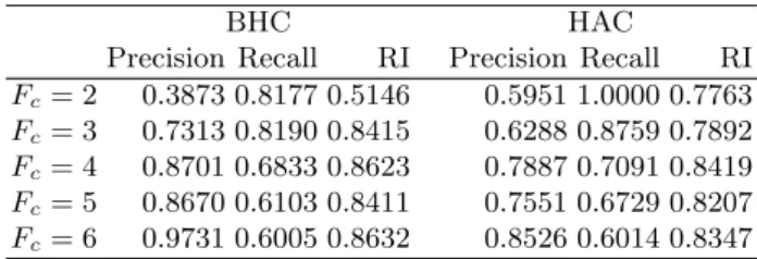
For this data set, we notice that for Fc= 2 and 3, the precision is low while the
recall is high. However, with the increasing of our cluster number, we notice that BHC provides a better results. In fact, for Fc = 3, 4, 5 and 6 the precision and
RI values relative to BHC are higher then the precision and RI values relative to HAC, which confirmed the efficiency of our approach which is better in terms of precision and RI.
Table 2.Evaluation results for Congressional Voting Records Data Set
BHC HAC
Precision Recall RI Precision Recall RI Fc= 2 0.3873 0.8177 0.5146 0.5951 1.0000 0.7763 Fc= 3 0.7313 0.8190 0.8415 0.6288 0.8759 0.7892 Fc= 4 0.8701 0.6833 0.8623 0.7887 0.7091 0.8419 Fc= 5 0.8670 0.6103 0.8411 0.7551 0.6729 0.8207 Fc= 6 0.9731 0.6005 0.8632 0.8526 0.6014 0.8347
6
Conclusion
Ultimately, we have introduced a new clustering method using the hierarchical paradigm in order to implement uncertainty in the belief function framework. This method puts the emphasis on the fact that one object may belong to several clusters. It seeks to merge clusters based on its pignistic probability. Our method was proved on data sets and the corresponding results have clearly shown its efficiency. The algorithm complexity has revealed itself as the usual problem of the belief function theory. Our future work will be devoted to focus on this peculiar problem.
References
1. Bezdek, J.C., Ehrlich, R., Fulls, W.: Fcm: The fuzzy c-means clustering algorithm. Computers and Geosciences 10(2-3), 191–203 (1984)
2. Denœux, T.: A k-Nearest Neighbor Classification Rule Based on Dempster-Shafer Theory. IEEE Transactions on Systems, Man, and Cybernetics - Part A: Systems and Humans 25(5), 804–813 (1995)
3. Denœux, T., Masson, M.: EVCLUS: Evidential Clustering of Proximity Data. IEEE Transactions on Systems, Man, and Cybernetics - Part B: Cybernetics 34(1), 95– 109 (2004)
4. ben Hariz, S., Elouedi, Z., Mellouli, K.: Clustering approach using belief function theory. In: AIMSA. pp. 162–171 (2006)
5. Hastie, T., Tibshirani, R., Friedman, J., Franklin, J.: The elements of statistical learning; data mining, inference and prediction. Springer Verlag, New York (2001)
6. MacQueen, J.: Some methods for classification and analysis of multivariate obser-vations. In Proceedings of the 5th Berkeley Symposium on Mathematical Statistics and Probability 11 (1967)
7. Masson, M., Denœux, T.: Clustering interval-valued proximity data using belief functions. Pattern Recognition Letters 25, 163–171 (2004)
8. Schubert, J.: Clustering belief functions based on attracting and conflicting met-alevel evidence. In: Bouchon-Meunier, B., Foulloy, L., Yager, R. (eds.) Intelligent Systems for Information Processing: From Representation to Applications. Elsevier Science (2003)
9. Shafer, G.: Mathematical Theory of evidence. Princeton Univ (1976)
10. Smets, P., Kennes, R.: The Transferable Belief Model. Artificial Intelligent 66, 191–234 (1994)
11. Zouhal, L.M., Denœux, T.: An Evidence-Theoric k-NN Rule with Parameter Op-timization. IEEE Transactions on Systems, Man, and Cybernetics - Part C: Ap-plications and Reviews 28(2), 263–271 (Mai 1998)