Antiproton and Antilambda Annihilations on Several Nucleons

PHYSICAL REVIEW C VOLUME 39, NUMBER 1 JANUARY 1989

Antiproton

and

antilambda

annihilations

on

several nucleons

J.

Cugnon and

J.

Vandermeulen

Uniuersite deLiege, Physique Xucleaire Theorique, Institut dePhysique au SartTilman,

B.

5,B-4000Li'ege 1, Belgium (Received 12 August 1988)

Antiproton and antilambda annihilations involving several nucleons at the same time areassumed and arguments in favor ofsuch processes are discussed. A statistical model for annihilation on one

orseveral nucleons isstudied. Itisshown to give very good results for annihilation on one nucleon. The predictions ofsuch a model for annihilation on several nucleons are discussed extensively. The most important ofthose is the enhancement ofthe strange particle yield. Other predictions are

3 made forremarkable two-body channels and in particular for the mesonless annihilation n

_He~pp.

A geometrical model ismade to estimate the probability ofhaving annihilation on several nucleons in nuclei. Finally, the relationship between our statistical approach and current dynamical models lsdiscussed.

I.

INTRODUCTION

The possibility

of

annihilating an antiproton on more than one nucleon in atomic nuclei, suggested already a long time ago,' has received more and more attention in recent years, especially because

of

the appearance

of

new data that seem to require this phenomenon.

Furthermore, in previous papers, '

we tried to single out the main features

of

a two-nucleon annihilation process using a simple statistical approach and showed that strangeness production is enhanced compared to what it is for antinuclon-nucleon annihilation. Here we give

more detail about the model and discuss new features. Actually, our purpose is fourfold. First, we want to ex-tend it to

B

&1 annihilations (here

B

represents the

baryon number

of

the annihilating system), paying atten-tion to strangeness production. Second, we discuss the relative probability

of

the various

B

values and study a

simplified geometric model for estimating this

probabili-ty. Third, we make specific predictions fortwo-body final states, in particular for n He

—

+pp. Fourth, we investi-gate properties

of

B

=0

as well as

B

)

0 antilambda an-nihilations.

The basic premise

of

our approach is that antiproton annihilation is a complicated process, which, therefore, can be handled by a statistical approach.

It

has been known for a long time that the main features

of

antiproton-proton annihilations at rest and at low

momentum (especially the yields

of

the pionic final states) are largely consistent with such an assumption. ' Al-though it is clear that there exists some deviations from the statistical picture in antiproton-proton annihilation, ' it is certainly interesting to see what are the predictions

of

the statistical approach to

B

)

0

annihilations. Ulti-mately, the predictions may be used to reveal the ex-istence

of

B

)

0

annihilations and possibly to evaluate their frequency.

The paper is organized as follows. Section

II

contains a description

of

the statistical model that we used and

of

its main predictions and features.

It

is a microcanonical approach in the sense that energy and baryon number are

II.

THESTATISTICAL MODEL

For

B

=0

annihilations, our statistical model is embo-died by the following frequency distributions for, respec-tively, n-pion and

(KK+

l)-pion events:

fo(nm.

)=

Ao(ACO)"

'R„(

s;nm

), n

~2,

f

o(KK,

l~)

=

_{AOPs(AsCO)'+'Ri+2(}

_s;2mk,

lm ), l

0

.

(2.1)

(2.2)

In these equations,

R,

is the statistical bootstrap phase space integral. ' The dimensional constant

Co=(4nm

) plays a role similar to the interaction

volume in the original Fermi statistical model. ' The

normalization constant Ao ensures that all the frequen-cies sum up to unity. The free parameter A,is directly

re-lated to the average value

of

n,

.

It

should be close to one

if

the interacting system has a typical hadronic linear di-mension,

i.e.

,

-m

'.

It

turned out to be necessary to in-troduce two additional free parameters, As and

_ps

to

reproduce the fine detail

of

strangeness production.

Roughly speaking,

ps,

that we call the hindrance factor,

determines the relative yield

of

kaonic to pionic annihila-tion, and A,

_s

is moderately dependent upon

(

I

)

(in Ref. 4,

Xs was taken equal to A,). The quantity A._sCO can be

ten-tatively interpreted as the interaction "volume" for

strangeness production events, which may be diAerent

conserved exactly. In Sec.

III,

we discuss the relative probabilities for various values

of

B

in a given nucleus. We study a simple geometric model to estimate these probabilities and single out the main physical parameters which determine these probabilities. In Sec. IV, we

present our estimate for remarkable decay channels, like two-body final states. Section V presents an extension

of

our approach to antilambda annihilations. Finally,

Sec.

VI contains a discussion

of

the model and its relationship

tomore dynamical approaches.

F

=

_g

fo(nor),

tl=2 (2.3)

(n

)

=F

'

g

nfo(nor),

l2—2 (2.4)

(l

)

=(1

F)

—

'

g

lfo(KK,

l~),

1=0

whose experimental values are the following

F

=(95.

4+1)%,

(n

)

=5.

01+0.

23,

(l

)

=1.

95,

for an-nihilations at rest.

It

should be stressed, however, that

the statistical model, described above, reproduces fairly from the one leading topurely pionic final states.

In practice, the parameters A._,

ks,

_Ps are fitted to the

following observables:

well many more properties

of

antiproton-proton and antiproton-neutron annihilations, including the multipli-city distributions. We thus want to extend it to

8

)

0 an-nihilations and to analyze its predictions.

In our recent work, a fit was realized with A.

=1.

40,

As/A.

=1.

80, and

/3s=0.

22 [in our present notation, see

Eq. (2.

2)].

However the parameters can be varied to

some extent (in a correlated way) and still give an

accept-able fit. Our best fit is obtained with A.

=

1.

40,

As/A,

=

1.

80, and Ps

=0.

18.

The sensitivity

of

the branching ratios to nonstrange and

KK

channels is roughly given in Fig.

1.

The sensitivity is slightly larger

forbranching ratios to channels containing an hyperon.

For

B

)

0

annihilations, the generalization

of

Eqs. (2.1)

and (2.2) isprovided by the following equations:

fs(BN,

n~)=

Aii(ACii)

+"

'Rs+„(&s;Bmz,

nm„),

n

~

2

—

B,

n

~0,

fs(BN,

KK,

ln)=

Asks(lsC&)

+

'R

s+&(& sBm&,2m&,lm

),

l

~0,

fa((B

l)N

YK

p~)

Aa/3s(~sCa)

Ra+p

i(

s;Bmx,

2m'

pm

),

p

~0,

fs((B

—

1)N,

:-,

2K,

qa)=

A&Ps(ksC&)

+~+'Rs+ +z(Vs;(B

—

l)mz,

m-,

2mK,qm ), q

~0

.

(2.6)

(2.7)

(2.8) (2.9)

keeping on with the idea

of Ref.

18that the interaction volume is proportional to the mass

of

the initial system. We also retained the idea that /3, is the hindrance factor

for producing strange quarks. Thence, the factor

_P,

ap-pearing in the

Eq.

(2.9), since this channel requires the

creation

of

two ss pairs. Table

I

shows the predicted rates for

8

=1

—4annihilations, using the same set

of

pa-rameters asfor

8

=0.

The striking result is the enhancement

of

strangeness production in

8

)0

annihilations compared to

8

=0.

Note that the enhancement is basically due to the

chan-nels containing YK, while the

KK

channels are depleted. As we explained in

Ref.

4, this is a purely kinematical e6'ect. The possibility

of

YK lowers the strangeness pro-duction threshold energy as compared to

KK. To

quanti-fy the strangeness enhancement, we plotted in

Fig.

1, the percentage

of

nonstrange channels,

mls=

g

fs(BN,

n~),

(2. 10) and also the quantity,

n

(s)+n

(s)

n(q

)+

(n(q)

—

3B)

(2.11)

which represents the abundance

of

strange quarks rela-tive to nonstrange (q

=u,

d) quarks. This ratio, in the

The symbol Ydenotes a A or a X hyperon. Here we

have written down isospin averaged formulae. We limit ourselves to the channels described above, but we checked that channels containing

KKK

or two Y hype-rons, when possible (for

B

=2,

3,. .

.

,

e.

g.) represent less

than

1%.

InEqs. (2.6)—(2.9),we took Cs

=[(B+2)/2]

~

Co,

present case equal to n

(s)/n(q),

is directly. comparable

to thermal models for quark production in quark-gluon plasma and also in hadronic matter.

For

8

=0

and 1, one has

fo(KK

)

(n

)+

fo(KK)

(2.12) and

f,

(NKK)+

f,

(AK)+

_f,

(XK)+2f,

(:-KK)

(

n

)

+

f,

(NKK ) (2. 13) and similar expressions for

B

)

l.

In Eqs. (2.12) and (2.13),we use short hand notations: forinstance,

f

o(KK)

stands for the summation

of

fo(KK,

ln)

for all the values

of

l and

(n

) is the average number

of

pions in purely pionic channels. Figure 1shows that the number

of

non-strange channels substantially decreases when going from

B

=0

to

8 =

1but tends to stabilize forfurther increasing values

of

B.

On the other hand the strangeness content

continues to increase, at a slower pace however, when

8

increases. This is mainly due to the fact that the average number (n )

of

pions isdecreasing. As we said, the great change from

8

=0

to

8

=

1 arises from the possibility

of

production a AK pair instead

of

leading to NKK.

For

B

)

0, the available energy has to be shared between creating mesons and providing the kinetic energy

of

the

8

baryons. This explains why the pion multiplicity

regular-ly decreases with

B.

In particular, while the average number

of

pions (for any kind

of

final states) decreases regularly with

B,

the total number

(N

)

of

particles keeps increasing almost. linearly. We also study an extension

of

this model to in-Aight annihilations. At small antiproton

39 ANTIPROTON AND ANTILAMBDA ANNIHILATIONS

ON. .

. 183

nonstrange

yield

0.

9

0.

8

0.

7 0 1 2 3 4

I~

fm

0.

10

i

0.

08

0.

06

strangeness

content

(b)

II

o.

04

0.

02

0.

00 0

{a)gives the fraction ofnonstrange _{channels q} [con-taining only pions, and nucleons for

8

&_{0,Eq.(2. 1{))]as a}

func-tion of the baryon number

8

of the annihilating system. (b) gives the strangeness content Rs [measured in terms ofnumber ofquarks in the final states, Eq. {2.11)].In each case, the solid symbols refer to the best fit parameters _Ps, A.,and A._s indicated in the Table Icaption. The open symbols correspond to values ofthe parameters giving a less good but still acceptable fit for

B

=0.

momentum _p~,b, the main feature is the increasing

of

the available

c.

m. energy. But _{when p~,}

„)

2 GeV/c, one has

to refine the model to cope with two experimental facts:

(1) the average number

of

pions

(n )

increases more

slow-ly than calculated with Eqs. (2.1)and (2.2),which roughly predicts a linear increase with s; (2) the proportion

of

kaonic annihilations increases less rapidly than predicted

by Eqs. (2.1)and (2.2). However, the statistical approach should not be rejected. Indeed, the emitted pions are

fairly isotropic for a rather large domain

of

_p&,b.' There-fore, we propose to adopt the following generalizations:

(a) the interaction "volume" _Co should be taken energy dependent as in

Ref.

20, Y) O c5 O ~~ 0 2 0 &D 50

c

E II 0 C a5 v2 0 Q II ch

+

_i

&D 0 0 2 bQ c5 ce ~ Q cA CP V Q Q OO Q Q Ch Q Q Q Q m ' Q

~

Q Q Q Q Q Q Q Q Q Q Q QQ QQ OO Q QO Q Q Q QQ QQ Q Q Q Q Q QQ QQ QQ OO Q Q OO Q Q Q Ch Q OO QOO Q Q Q rt Q rt Q & Q t Q

Co(s)

_=h

~o 1ns

(s)

=

Co(so) s lnso (2.14)

where

so=4M,

M

being the nucleon mass. This

corre-sponds roughly to a reduction

of

the interaction volume as s [in units

of

GeV in

_Eq.

(2.14)] increases; (b) the quantity _p

=

A,_&/A, istaken tobe energy dependent as

p(s)=1+[p(so)

—

1]h(s)

. (2.15)

The first modification looks physically plausible, sirice the interaction time is expected to decrease with the in-cident energy. The second modification is equally

accept-able, since it is reasonable to admit that at high energy a symmetry is progressively restored between the role

of

mesons

of

different mass (7r,K) In .any case, the modifications (2. 14) and (2.15) provide a good description

of

the antiproton-proton experimental data up to about

10 GeV/c, as it is shown in detail in Refs. 20and

21.

We give in

Fig.

2 the variation

of

the

KK

production

yield and compare it with experiment. Togive an idea

of

the importance

of

the modifications (2.14) and (2. 15) the predicted yield at 6GeV/c would be

0.

38

if

the latter

were removed.

The main prediction

of

this extended model is

con-tained in Fig.

3.

As energy increases, for

B

=0,

the

num-ber

of

s quarks and the number

of

_q quarks steadily

in-crease. Their ratio is moderately increasing: it is more and more easy to create

KK

pairs.

For

B

=1,

both num-bers are increasing, but their ratio, after rising to a

max-imum at

p„b=4

GeV/c, slightly decreases. We explain this effect as follows. The pion production is somehow hindered by the possibility

of

the AKchannel. As the en-ergy increases, the hindrance is less effective because one goes more and more away from the threshold. As

Fig.

3

shows, the increase

of

strangeness production with

ener-gy is nevertheless substantial. At 6 GeV/c, in

B

=1

an-1.

0 ~E

nonstrange

yield

0.

9

0.

&-0.

V P

0.

6

0.

5 2 4 6

p

{Ge~/c}

nihilations, the yield

of

strange channels reaches

50%

and then keeps increasing very slowly.

We also calculated many quantities in addition to the yield.

For

instance, in

Fig.

4, we show the energy spec-trum

of

various particles.

For

B

=0,

the pions appear thermal-like with a temperature

of

T

=110

MeV. This temperature is lowered a little bit when one goes from

B

=0

to

B

=1.

This is so because the available energy should be shared to more particles. The spectrum

of

the nucleons in

B

=1

strikingly shows the inhuence

of

the

microcanonical approach since the change

of

slope

corre-sponds to nucleons at the edge

of

the available phase

space compatible with the energy-momentum conserva-tion law. The difference between nucleon and hyperon shapes comes from the fact that in the latter case, one is

almost at the edge

of

phase space even for slow moving hyperons. This comes from the part

of

the available en-ergy which is transformed in mass. This situation also applies to the kaon spectrum for

B

=0.

The difference

of

temperatures

of

pions and slow

("

canonical'*) nucleons can be explained by the fact that our model is not a stan-dard thermal model as far as pions are concerned.

Indeed, the model neither assumes a constant number

of

strangeness

content

C:

g

0.

2-tw D 1

g

5

l~

Ice Il Cl 2

B=O

~I 2 4 p _& (GeV/c) 0 0 I a I 2 4

p

(Gev/c)

.

FIG.

2. Comparison ofthe K%I~branching ratio as

calculat-ed inthis paper (curve) with the experimental data ofRef.22.

F&D.3. Evolution ofnonstrange yield (upper part) and ofthe strangeness content (lower part), both in

8

=0

(solid symbols) and in

B

=1

annihilations (open symbols), as a function ofthe incident momentum p~,bofthe antiproton.

39 ANTIPROTON AND ANTILAMBDA ANNIHILATIONS

ON. . .

I8S 10 000 A—1

PsrsDs,

B=0 (3.1) 1000 100 10

0,

00 10 000 1000

0.

20

0.

40

0.

60

I-m

{QeV)

0.

80

where PB denotes the probability that the annihilation

occurs on

(8

+1)

nucleons,

_rs

is the branching ratio for

the particular class

of

events in that case, and DB represents the distortion due to the subsequent cascades. In most cases, it simply is an average absorption coefficient.

The most di%cult task is,

of

course, the computation

of

DB which requires an elaborate cascade calculation. We

here concentrate on the probabilities PB, for which one may build a simple geometrical model for annihilation in Aight. We assume that the incoming antiproton forms with a nucleon a

B

=0

fireball which can decay with some lifetime ~o, but which can form a

B

=1

fireball,

pri-or to that,

if

it encounters another nucleon. We call cr&

the associated cross section. The

B

=1

fireball is provid-ed with a lifetime ~, and a cross section o.

2 for forming a

B

=2

fireball, and so on.

To

simplify the calculations, we

rely on the Glauber picture

of

a forward motion. The

model may be put in the form

of

rate equations le A ie 100 10 dQo(z)

₌

_—

~op(z)

Qo«»

dZ dRo(z)

₌

oop(z)Qo(z)—

dZ Tovo&o

(3.

2a)

+o,

p(z)

Ro(z),

(3.2b) ,1

0.

0

0,

2

0.

4

0.

6

0.

8

1.

0

1.

2 E-m (QeV) and dR, (z)

=o,

p(z)R, ,

(z)—

dz _{7l i} i L

+

o.

_;+,

_p(z)

_R;(z),

FIG.

4. Energy spectrum

f

(E)

for various emitted particles,

both for

B

=0

and for

B

=1

annihilations. The spectrum is di-vided by the product ofthe momentum by the total energy. In this representation a thermal spectrum appears as a straight line. Temperatures are tentatively extracted and displayed.

pions nor a constant chemical potential.

The change

of

slope at the extreme tail

of

the spectra,

especially for

B

=0,

is due to the contribution

of

the three-body decay (the two-body is not included in the figure), while the main part is due mainly to n-body de-cays, with n

~4.

Other quantities, like, for instance, the shape

of

the multiplicity distributions, show interesting variations

when

B

is changed, but one can say, in conclusion, that

none shows a qualitatively important change as the strangeness yield.

III.

NUCLEAR EFFECTS

The important issue is to detect the existence

of

B

&

0

annihilations in antiproton annihilation on a nucleus.

Let us suppose we focus our attention on a special kind

of

event.

To

fix the ideas, this may correspond tothe

detec-tion

of

a

K+.

In all generality, the yield per annihilation

for such kinds

of

events, on a target

of

mass number

3,

can be written as

(3.

2c) fori

=

1,2, .

.

.

,n. Here, zisthe coordinate along the tra-jectory

of

the antiproton or its subsequent fireball inside

the nucleus; U,- isthe velocity

of

the

B

=i

fireball and

y, is the associated Lorentz factor. The quantity

ao

is the

_pX

annihilation cross section. At

z= —

~,

the probability

Qo

of

having an antiproton is equal to unity and the

probability

R,

-

of

having a

B

=i

fireball isvanishing. The

connection between the quantities

Ps of

Eq. (3.1)and the functions

Rs(z)

is given by

PB=

lim

I

(yiiusrs

) 'Rii(y)dy

1

—

_Qo(z)

(3.

3)

The use

of

the Glauber picture is more or lessjustified

by the fact that the latter provides a surprisingly good description

of

the antiproton reaction cross sections. The predictions

of

this model should not be taken too

seriously: it is aimed at providing rough estimates

of

the

PB's only. In particular, only reasonable guesses

of

the quantities w, and

o,

(i

)

1)are available. We give in Fig. 5 the decay rates

of

the fireball

of

baryon number i

[i.

e.,

the term containing the

r,

in Eqs. (3.2b) and (3.2c)]in a typical example and with typical parameters o._,- _cT

p

0.

12

181

p (4GeV

jc)

+

Ta

0.

80 181

p

(4 GeV/c) +

Ta

0.

10

0.

08

0.

06

0.

04

0.

02 Q D B=O D D D

1

L 0 2

0.

60,

0.

40

0.

20

0.

00 —

₁₀

₁₀

0.

000 z (Km)

FICr. 5. Evolution as a function ofthe distance zofthe decay probability for the fireballs ofbaryon number

B

=0

to 3, respec-tively, in the case ofcentral antiproton annihilation on Ta nu-cleus. The target nucleus iscentered atz

=0.

same _p~,b dependence forall cross sections. The figure re-veals that most

of

the annihilations happen rather close

to the surface. There is, however, a slight shift from the average location

of

annihilations when

B

is going up. In

Fig.

6 we show the results

of

the same model when

different, but still reasonable assumptions are made for

the quantities o._; and ~,

.

In one case, we assumed that o._;

increases when iincreases, with a geometrical law

2

(8+I)'i

+1

0B

2 Oo (3.4)

Inthe other case, the lifetime isassumed todecrease with the mass number as

+B

_B+2

2 (3.&)

and

~o=1

fm/c. As one can see, these modifications do not influence the results dramatically. Therefore, we can safely conclude that on the basis

of

reasonable geometric assumptions, the annihilation rate for

B

&0

should be

of

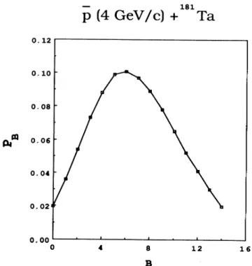
FICx.6. Distribution ofthe quantities I's [Eq. (3.1)] for cen-tral annihilation ofantiprotons on Tanuclei. The solid squares correspond too.;

=o.

oand ~;

=1

fm/c. The open squares are

ob-tained with Eq. (3.5)and the crosses with Eq. (3.4) (see the text for details).

the order

of

10%

in actual nuclei. However, it is not

likely to have very large values

of

B.

The most important parameter to favor large

B

isthe lifetime ~. But, we have increased the lifetime ~o up to 5 fm/c. We observed a maximum

of

PB at

B

=2

only, although the distribution is much broader. In

Fig.

7, we display the population probability for the baryon number

B

of

the fireball in the limiting case

of r,

—

+

~

[keeping Eq. (3.

4)].

In this case,

the fireballs grow up to a mass which roughly

corre-sponds to the number

of

nucleons intercepted by the

cross section o.oat that energy. This number turns out to be around

6.

The short-range correlations between nucleons limits the piling up

of

the fireballs. This can be accounted forin Eqs. (3.2b) and (3.2c) by multiplying p(z) in all terms

in-volving the quantities

R,

by the function

g(z)

which represents the probability

of

having two nucleons at a

distance z from each other. We checked that with reasonable forms

of

g(z),

this amounts to introducing an effective cross section about

60% of

the original o s.

Finally, we give in Table

II

the values

of

the probabili-ties

of

having various

B

annihilations on the nuclei He TABLE

II.

Probability P&ofhaving a

B

annihilation on 'He and He targets.

p~,b (GeV/c) 0.4 0.6 1 2 4 Po 0.900 0.886 0.873 0.868 0.882 'He Pl 0.088 0.100 0.110 0.114 0.105 P2 0.011 0.014 0.016 0.016 0.013 Po 0.885 0.866 0.846 0.836 0.849 Pl 0.099 0.113 0.128 0.136 0.128 4He P2 0.015 0.019 0.024 0.025 0.020 P3 0.00021 0.00043 0.00080 0.0014 0.0014

39 ANTIPROTON AND ANTILAMBDA ANNIHILATIONS

ON.

. .

187

0.

12

0.

10

0.

08

0.

06

p (4

GeV/c)

+

Ta

inTableEq.

III,

(3.

1)]thereis ispredictedan isospintofactor —be

4.

7X10

',). A comparison(relative

to

of

formula

(3.

1) with the experimental rate (Ref. 28),

(28+3)

X

10,

yields a probability P&

=(6+0.

6)% of

hav-ing

8 =

1 annihilations (in the case

of

kinematically

defined two-body decays, the distortion _{factors Dz} are equal to one). Taking this value

of

P„we

can make pre-dictions for pd

—

+A

K

and pd

~

X

K

yields,

i.e.

,

about

6X

10 and about

12X

10 per annihilation, re-spectively.

One may look at the predictive power

of

our model from another point

of

view. Indeed, the ratio

of

the

fol-lowing yields

0.

04 g(pd

~X

K+

) pi g(pd

~per

) (4.1)

0.

02'

0.

00 0

B

12

16

FIG.

7. Probability distribution ofthe baryon number

B

of the fireball [quantities R~in Eq. (3.2)] at the outcome ofthe tar-get in the limit of~&

~

~

(seethe text for details).

and He (which presents some cosmological interest ). In this particular case, we have summed over all possible impact parameters, using standard assumptions and Gaussian density distributions with parameters taken from

Ref. 26.

These values will be used in

Sec. IV.

IV. TWO-BODY EXITCHANNELS

The most convincing fact in favor

of

B

&

0

annihila-tions is the observation

of

two-body decays (with clear

kinematical signature) like the following one: pd

+pvr-We want here to present the predictions

of

our model for

this kind

of

process. Once again, we checked that the model works fairly well for

B=0

(see Table

III).

This

gives us some confidence in extending the model for

8

&

0.

Letus detail a little bit the results. A.

B=1

The branching ratio for pd

~pm

in

8 =

1 [quantity r&

is independent

of

the quantity P&

[Eq.

(3.1)],and tests the

statistical part

of

our model (Sec.

II).

Indeed,

_p,

writes

~s

Pr

pl

Is

Pp

(4.2) where

p*

denotes the

c.

m. momentum in the final state,

and is directly connected to the hindrance factor I3,

.

Similarly, the ratio

g(pp

~K+K

),

~s Pz

rj(pp sr+sr )

'

~

_p*

(4.3)

is proportional to the hindrance

factor.

The crucial step

in Sec.

II

is to assume that the hindrance factor is the same for

8

=0

and

B

=1.

Therefore, the quantities

_p,

and _p2 are really testing the model. In particular, the equivalence

of

the hindrance factors implies

p],

pr.

p~

Pp

Pz

(4 4)

The value

of

the right-hand side for annihilations at rest is

—

1.

7.

The experimental value

of

_{p2 is} known to be

-0.

33.

Therefore,

if

our assumption iscorrect, _p& should be

of

-0.

28. Experimentally _p& is not known.

If

the

pd~pm.

yield is

(28+3)X10,

the

pd~X

K+

one should be

of

the order

of

(15+l.

5) X 10

.

This is to be compared with a

90%

confidence upper limit

of

about

SX10,

according to

Ref.

27. An improvement

of

this

TABLE

III.

Calculated and measured branching ratios for several two-body final states in various

B

annihilations. The liquid hy-drogen data are taken from the compilation ofRef. 17. The gas data are from Ref. 27.

Theory Expt. liquid gas 0.51 X 10 KK 0.14

x10-'

pp

~&

0.42 X10 (0.37+0.02) X10 (0.32+0.03) X10

B=0

pp

~K+K

0.07 X10 (0.

11+0.

01) X10 (0.096+0.008)

x10

'

pp~K

K 0.07

x10-'

(0.072+0.010)

x10-'

(0.

081+0.

005) X10 (0.

051+0.

012)

x10-'

N~ 7.06

x10-4

B=1

AK 1.03

x10-4

XK 3.00

x

10-4

B=2

NN 1.06

x10-4

measurement is clearly needed to confirm or infirm our

approach.

Let us note that the pd

—

+pm yield has recently been measured by another group which finds a rate

of

(14+7)

X10,

somewhat lower than the value

of

Ref. 28.

B.

B=2

This case isparticularly interesting since it corresponds

to

the emission

of

two nucleons without any meson: the so-called Pontecorvo reactions. ' There are four

of

them:

The most interesting ones are the first one and, perhaps

even more, the last one because the final state contains two charged particles. Combining the results

of

Tables

II

and

III,

we can make a prediction

of

the yield for this particular reaction. The latter turns out to be

of

the

or-der

of

10,

which seems to be just sufficient to make a measurement possible with the present beam and

detec-tion possibilities. Our prediction istobe contrasted with

the result

of Ref. 31,

where the authors give an estimate

of

10 —

10,

but using a very specific six-quark inter-mediate state. p

He~pn,

pt

~nn,

nt

~pn,

n

He~pp

. (4.5a) (4.5b) (4.5c) (4.5d) V. ANTILAMBDA ANNIHILATIQN

In the near future, experiments with antilambdas will

be possible with good statistics.

For

this reason, we

present here the results

of

our model for this case. The

corresponding expressions are then (for

B

=0)

fo(K, nm)=do(ACo)"R„+,

(

s;mx,

nm ), n

~1,

fo(KKK,

/~)=A

o(k sC o) +

R(+,

(

s;3m~,

lm ),

l~0,

and (for

B

=

1)

f,

(N K,nm')

= 3

_)(AC)

)"+'R„+2( s;m~,

m~,nm ), n

0,

f,

(N,

KKK,

le)=

Ai~s(~sCi)

Rt+4(+s

'mx, 3m'',

lm ), I

~0,

f)(Y,

KK~p~)=A)/3s(ksC,

) +

R„+3( s;my,

2m~,pm ), _p

0,

(5.1) (5.2)

(5.3)

(5.4)

(5.5)

for the most important channels. We used the same

values

of

the coefficients as before, as well as the same s dependence.

The results

of

the antilambda annihilation at rest are presented in Table IV and compared to

the,

antinucleon annihilation case. One can realize that the rates for the corresponding channels in the two cases (both for

B

=0

and

B

=1)

are very similar. The multiplicities are

slight-ly smaller in the antilambda case compared to the antinu-cleon case. This is understandable in view

of

the fact that strangeness conservation imposes the presence

of

a

K

meson in the final state, which requires more energy than the lambda-nucleon mass difference.

The

B

=1

antilambda annihilation leads also to the

TABLE IV. Upper part: branching ratios in

%

for several types offinal states and associated aver-age pion multiplicities in

8

=0

and

8

=1

annihilations ofantinueleons and ofantilambdas. Lower

part: average multiplicities for various particles.

B=0

NN NNN ANN (N„& &N ) (N~ ) &N )

(N.

)

(N,

) &N& (n& KKlm. 95.34 4.90 4.66 1.85 4.76 0.047 0.047 4.85 Kn~ (n& KKKlm

(i)

96.47 3.57 3.53 0.54 3.46 1.035 0.035 4.53 Nn~

(n)

NKKlvr &I) AKp

~

(p)

XKp'~

(p')

82.94 4.57 3.76 1.45 4.79 2.69 8.49 2.68 4.21 0.17 0.038 0.867 0.048 0.085 5.42 NKn

~

(n)

NKKKlm

(»

AKKpm

(p)

2K''w

(p')

86.76 3.21 2.37 0.32 3.93 1.45 6.94 1.25 2.93 1.14 0.024 0.891 0.039 0.069 5.09

39 ANTIPROTON AND ANTILAMBDA ANNIHILATIONS

ON. .

. 189

TABLE V. Comparison of the calculated NNN~Nm. and ANN~NK branching ratios as a function of the incident momentum. 0 0.5 1 2 3 4 5 6 7.06

x

10-'

4.

79x10

4 1.99

x

10-'

2.88X10 5.28X10 1.34X10 4.28

x

10-'

1.64

x

10-'

ANN

~NK

1.46

x

10-'

1.07

x

10-'

5.08

x

10-'

7.

81x 10-'

1.23X10 2.86

x

10-'

8.15

x

10-'

3.10X10

VI. DISCUSSION, CONCLUSION

In this work, we proposed a picture

of

the annihilation

process, which can be characterized by the following

features:

(1) Thefinal state probabilities proceed from a statistical picture. The underlying assumption is that the

annihila-tion process is a rather complicated process, which in-volves a strong rearrangement

of

the parton structure. Therefore it is very much alike the compound nucleus formation forthe nucleons.

(2) The annihilation on seueral nucleons occurs whenev-er possible. Again, this assumption derives from the

ob-servation that the fundamental process is the quark-antiquark annihilation.

(3) The statistical picture applies toall annihilations, in-cluding those involving more than one nucleon.

(4)Strangeness production is hindered Furthermo. re, it isassumed that the hindrance is the same for all kinds

of

annihilations, irrespective

of

the number

of

nucleons in-volved.

This approach works very well for

B

=0

annihilations.

This statement pertains to points (1)and (4) above. We have avery good reproduction

of

the branching ratios for

many final states,

of

the pion multilicity distributions,

of

the pion spectrum,

of

the strangeness production yield,

etc.

This isobtained with the help

of

only three free pa-rameters (for annihilation at rest). This part

of

our

ap-proach seems very successful. We think that such a suc-cess is not accidental and that the model should cover the

correct physical picture. We have toadmit however that

points (2)and (3) have not yet been tested up

to

now, even

though there are experimental indications in favor

of

the annihilation on several nucleons. ' _{The very}

observa-possibility

of

remarkable two-body channels. In particu-lar, the following reaction Ad

~K

_p isallowed. W5 give

in Table V the relative rates for

B=1

annihilation in Right leading to two particles in the final state, both for

antilarnbda and for antiproton. The branching ratios

vary in a fairly similar way as a function

of

the incident momentum. Taking into account isospin weights, we predict

rt(Ad~@

p)

rt(pd~vr

p)

tion

of

the pd

~p~

reaction ' _{strongly suggests that}

the annihilation process involves two nucleons at the same time.

It

should not be considered as aproof for the time being, since it can also be pictured as due to the reabsorption

of

an off-shell pion by the second nucleon. However, it is not sure that the two approaches exclude each other and that they are not merely two descriptions

of

the same physical reality using different words and different degrees

of

complexity. Analyses

of

various strangeness yields seem to call also for the need

B

&

0

an-nihilations as itisshown in

Ref. 35.

An interesting question is to know whether our

ap-proach bears some relationship with the current

dynami-cal approaches using the quark structure.

To

summarize

very brieAy the situation with the latter, ' ' _{one can say} that there are two basic philosophies. In one case, it is

assumed that the quark-line diagrams should be ordered with increasing number

of

annihilation and/or creation

quark-antiquark vertex. In the other one, on the con-trary, they should be ordered with decreasing character

of

planarity. Obviously, our statistical model is more closely related to the so-called annihilation diagrams, which are sketched in Fig. 8(a). More precisely, our ap-proach consists in retaining this class

of

diagrams and in

identifying the intermediate state [dotted line in Fig.8(a)] as a heavy meson which decays statistically. This

con-nection assumed between meson decays and annihilation

process should reAect in a similar mean multiplicity

of

final products. We show in

Fig.

9(a),as a function

of

the

N I

(a)

N N

(b)

FICx. 8. (a) "Annihilation" diagram for

B

=0

annihilation', (b) possible "annihilation" diagram for

8 =1.

See the text for details.

mass, the mean multiplicity in the pionic modes

of

antiproton-proton annihilation at rest and in the decay

of

the nonstrange mesons which have dominant pionic channels.

It

is seen that the linear dependence connect-ing the pion to the antinuclon-nucleon system goes through the meson points in the mass domain around

10

{a)

nonstrange rnesons

A

g

V 6 0 0 I 1 m

_{GaV)

(b}

baryonic

resonances

6 2 0 0 I R I 2 m

{GeV)

6

(c}

strange rnesons 0

0

I 1 m

{GaV)

FICr. 9. Multiplicity ofstable products (m, K,N, and y from q) in the decay ofvarious systems: (a)

S

=0

mesons (diamonds and squares, the latter corresponding to the decays involving g's) and antiproton-proton at rest (open circle). (b)

S

=

0

baryons (solid diamonds and squares) and (NNN) system at rest (open diamond). (c)

S

= —

1 mesons (squares) and antilambda-nucleon system at rest (open diamond). The open diamonds are our theoretical results while all the other points are experimen-tal ones, taken from Ref. 37 or from Ref. 17for the open circle inpart (a).

about 1 GeV; beyond about

1.

3GeV, the identified reso-nances tend to cluster below the line, the result

of

a prob-able bias favoring the identification

of

states with low final mean multiplicities. Some states with the

_g

meson as a main decay product are known [squares in Fig. 9(a)]

and it is obvious that channeling through _g makes the system more easily identifiable than for a set

of

more loosely correlated particles.

Once the picture

of

a mesonlike intermediate state is accepted, some other features

of

our approach arise natu-rally. First, strangeness production requires a ss creation

vertex, whose importance is reduced in comparison with

a qq vertex because

of

the mass

of

the strange quarks. Second,

if

two nucleons are close enough, it is reasonable

to admit that an antiquark in the antinucleon annihilates with a quark in one nucleon bag while another antiquark annihilates with a quark

of

the other nucleon bag, which corresponds to an annihilation on two nucleons. One possible graph for this process isdepicted in Fig. 8(b).

Fi-nally, it is natural within this scheme to assume that

strangeness production is reduced in the same manner in

B

=0

and

B)0

annihilations. Let us notice, however, that within this simpleminded quark picture,

B

should be limited to 0, 1, and 2.

A test on final multiplicity similar to the one for

B

=0,

can be made with the observed nucleon resonances and our prediction for

8

=

1annihilation. As Fig.9(b) shows, the decay multiplicities

of

the resonances

of

X"

and

6*

type cluster around the line joining the nucleon to the

B

=

1 system.

It

is also instructive to consider the strange systems with

8

=0.

We have plotted in Fig. 9(c)

the experimental figures for the mean product multiplici-ty

of

the strange mesons and our prediction for

antilambda-nucleon annihilation at rest. The connection works out amazingly well here

too.

One

of

the surprising results

of

our analysis is that it

gives a reasonable yield for the rare channels,

i.

e.

, in a sector where astatistical approach is sometimes expected

to fail. This definitely applies in

B

=0

annihilations. In

that respect, it is interesting to mention that the double production

of

a

I| K

pair seems to be predicted at the right order

of

magnitude by our model, which includes

/3s as factor in that case. At

3.

66 GeV/c the measured

cross section for

_{pp~2K2Kja (j}

0) is (3.1+2 3)10

mb. We find a fraction

of

9X10

which, multiplying a

total annihilation cross section

of

=30

mb gives a

pre-dicted cross section

of

=2.

7X10

mb. But the agree-ment between model and.experiment can also apply to

8 =

1 (see

Sec.

IV), provided a reasonable frequency

of

B

=1

events isassumed in thepd system.

The most important issue at present is to know wheth-er

8

=1

annihilations really occur in antiproton (or anti-baryon in general) annihilation on atomic nuclei. As we

said in the Introduction and in

Sec.

II,

the best indicator seems to be the strangeness production yield. This

of

course relies on our assumption for a hindrance _{factor Ps} independent

of

B.

As we explained in Sec. IV, this as-sumption can be tested on the ratio

_p,

/p2, which is

in-dependent

of

the frequency for

B

=

1 annihilations.

Therefore, accurate measurements

of

pd

~p~

and

Pd~X

K+

(and/or X

K,

AK )are desirable. With this

39 ANTIPROTON AND ANTILAMBDA ANNIHILATIONS

ON. .

.

assumption, one can analyze strange particle production and compare it to the expected yield in the presence

of

B

=0

annihilations only, as explained in Sec.

III.

In our previous works, we did such an analysis in some simple

cases. The _difhculty in this analysis is a correct estimate

of

the factors Dtt

[Eq.

(3.

1)]. For

the interesting case

of

p

—

Ta

at 4 GeV/c, we postpone this analysis to a forth-coming paper, where we will use the full complexity

of

the intranuclear cascade model. We here concentrate our attention on the factors

Pz,

which can be estimated by a geometrical model. We showed in Sec.

III

that

annihila-tion on two nucleons or more are expected to occur with a frequency

of

the order

of

10%. It

ishowever unreason-able to expect the appearance

of

an annihilating system involving really many nucleons at the same time, as it was suggested in

Ref. 38.

Let us finally emphasize that another check

of

the relevance

of

our approach is provided by the mesonless annihilations, and in particular by the n

_He~pp

reac-tion. We predict a non-negligible yield, which could be measurable in the near future.

tB. M. Pontecorvo, Zh. Eksp. Teor. Fiz. 30, 947 (1956)[Sov.

Phys.

—

JETP 3,966 (1957)].

J.

Rafelski, in Physics at LEAR, edited by U. Gastaldi and

R.

Klapisch (Plenum, New York, 1984).

3S. Kahana, Proceedings ofthe Workshop Physics at LEAR, edit-ed by U. Gastaldi and

R.

Klapisch (Plenum, Ne+ York,

1984),p. 495.

4J.Cugnon and

J.

Vandermeulen, Phys. Lett. 146B,16(1984).

J.

P.Bocquet et al.,Phys. Lett.B182,146(1986).

J.

P.Bocquet et al.,Phys. Lett.B192, 312 (1987).

7M. Miyano et al.,Phys. Rev.Lett. 53,1725(1984).

J.

Cugnon and

J.

Vandermeulen, Phys. Rev. C 36,2726(1987).

C.

J.

Hamer, Nuovo Cimento A 12,162(1972).

~oS.

_J.

Orfanidis and V.Rittenberg, Nucl. Phys. B59,570(1973).

J.

Vandermeulen, Lett.Nuovo Cimento 11,243(1974). H.Mohring et al.,Nucl. Phys. B85,227(1975).

B.

Margolis, W.

J.

Meggs, and N. Weiss, Phys. Rev. D 13,

2551(1976).

C.Dover, in Proceedings ofthe Third Conference on the In-tersections Between Particle and Nuclear Particles,

Rock-port, 1988 (AIP,New York, tobe published).

~5R.Hagedorn and

I.

Montvay, Nucl. Phys. B59,45(1973).

E.

Fermi, Prog. Theor. Phys. 5,570{1950).

R.

Armenteros et al., CERN Report No.

CERN/PSCC/80-101, 1980).

R.

Hagedorn,

I.

Montvay, and

J.

Rafelski, in Hadronic Matter

atExtreme Energy Density, edited by N. Cabibbo and L. Ser-torio {Plenum, New York, 1980), p.49.

P.Gregory et al.,Nucl. Phys. B102,189(1976).

oJ.Vandermeulen, Lett.Nuovo Cimento 28,60(1980).

J.

Vandermeulen, Lett.Nuovo Cimento 21,33(1978). H. Muirhead and P. Gregory, Antinucleon-nucleon

Interac-tions, edited by G.Ekspong and S.Nilsson (Pergamon, New

York, 1987), p.331.

~3F. Balestra et al.,Nucl. Phys. A452, 573(1986).

~4A. _{Lejeune, P. Grange,} M. Martzolff, and

J.

Cugnon, Nucl. Phys. A453, 189(1986).

V. M.Chechetkin, M. Yu.Khlopov, M.G.Sapozhnikov, and Ya.

B.

Zeldovich, Phys. Lett. 118B,329(1982).

26H. Uberall, Electron Scattering from Complex Nuclei, Part A

(Academic, New York, 1971),Chap. 5.

S.Ahmad et al., Physics with Antiprotons at LEARin theAcol

Era, edited by U.Gastaldi et al. (Editions Frontieres, Gifsur Yvette, 1986), p.353.

~sCJ.A.Smith, in The Elementary Structure ofMatter, edited by

J.

M.Richard et al.(Springer-Verlag, Berlin, 1988), p. 197.

This corrects our estimate of Ref.4, where an isospin factor

had been neglected.

J.

Riedlberger et al.(ASTERIX Collaboration) Nucl. Phys. C

(to be published).

'L.

A. Kondratyuk and M. G.Sapozhnikov, Physics at LEAR

with Low Energy Antiprotons, edited by C. Amsler et al.

(Harwood-Academic, New York, 1988), p.771. 3~R. Bizzarri et al.,Lett.Nuovo Cimento 2,431(1969).

B.

Y.Oh et al.,Nucl. Phys. B51,57(1973).

34E. Oset, Physics at LEAR with Lour Energy Antiprotons, edited by C.Amsler et al. (Harwood-Academic, New York, 1988), p.753.

35J. Cugnon, in TheElementary Structure

of

Matter, edited by

J.

M.Richard et al.(Springer-Verlag, Berlin, 1988),p.211.

J.

M. Richard, in Proceedings ofthe Third Conference on the

Intersections Between Particle and Nuclear Particles,

Rock-port, 1988(AIP, New York, tobe published). Particle Data Group, Phys. Lett. 170B,1(1986).

J.

Rafelski, Phys. Lett. 207B,371(1988).