Éléments finis solide-coque pour l’analyse quasi-statique et dynamique des structures minces 3d : application aux procédés de mise en forme

(1)

HAL Id: tel-01540345

https://pastel.archives-ouvertes.fr/tel-01540345

Submitted on 16 Jun 2017

HAL is a multi-disciplinary open access archive for the deposit and dissemination of sci-entific research documents, whether they are pub-lished or not. The documents may come from teaching and research institutions in France or abroad, or from public or private research centers.

L’archive ouverte pluridisciplinaire HAL, est destinée au dépôt et à la diffusion de documents scientifiques de niveau recherche, publiés ou non, émanant des établissements d’enseignement et de recherche français ou étrangers, des laboratoires publics ou privés.

et dynamique des structures minces 3d : application aux

procédés de mise en forme

Peng Wang

To cite this version:

Peng Wang. Éléments finis solide-coque pour l’analyse quasi-statique et dynamique des structures minces 3d : application aux procédés de mise en forme. Mécanique des matériaux [physics.class-ph]. Ecole nationale supérieure d’arts et métiers - ENSAM, 2017. Français. �NNT : 2017ENAM0010�. �tel-01540345�

(2)

Arts et Métiers ParisTech - Campus de Metz

Laboratoire d’Étude des Microstructures et de Mécanique des Matériaux (LEM3) UMR CNRS 7239

2017-ENAM-0010

présentée et soutenue publiquement par

Peng WANG

le 6 avril 2017

Solid



shell finite elements for quasi-static and

dynamic analysis of 3D thin structures:

Application to sheet metal forming processes

Doctorat ParisTech

T H È S E

pour obtenir le grade de docteur délivré par

l’École Nationale Supérieure d'Arts et Métiers

Spécialité “ Mécanique - matériaux ”

T

H

È

S

E

Jury

M. Jean-Philippe PONTHOT, Professeur, LTAS, Université de Liège, Belgique Président M. Laurent DUCHÊNE, Professeur associé, ArGEnCo, Université de Liège, Belgique Rapporteur M. Thomas ELGUEDJ, Maître de Conférences  HDR, LaMCoS, INSA de Lyon, France Rapporteur M. Olivier POLIT, Professeur, LEME, Université Paris Nanterre, France Examinateur M. Habibou MAITOURNAM, Professeur, IMSIA, ENSTA ParisTech, France Examinateur M. Farid ABED-MERAIM, Professeur, LEM3, Arts et Métiers ParisTech, France Examinateur M. Hocine CHALAL, Maître de Conférences, LEM3, Arts et Métiers ParisTech, France Examinateur

Directeur de thèse : Farid ABED-MERAIM Co-encadrement de la thèse : Hocine CHALAL

(3)

(4)

To my beloved parents for their sacrifices

To my beloved sisters and brothers for their support

To my dear supervisors for their guidance

To all my dear friends for their help

(5)

(6)

Acknowledgments

This work has been realized within the team MeNu (Mécanique Numérique) of the laboratory LEM3 (Laboratoire d‘Étude des Microstructures et de Mécanique des Matériaux) in Metz Campus of ENSAM (École Nationale Supérieure et d‘Arts et Métiers). The study in France was a valuable and memorable experience in my life. First and foremost, I would like to thank my supervisors for their dedicated support, kind guidance and encouragement.

I sincerely thank the director of my thesis, Prof. Farid ABED-MERAIM, who kindly gave me this opportunity to study in France. I am deeply grateful for his encouragement, invaluable advices and guidance during my study. I would like to thank my co-supervisor, Dr. Hocine CHALAL, for his responsible supervision, meticulous guidance and kind assistance. Without them, it is impossible for me to complete this thesis on time. It was a really great pleasure for me to work with them for three years.

I also deeply thank Prof. Jean-Philippe PONTHOT from Université de Liège for being the president of my Ph.D. thesis committee. I would like to express my gratitude to two reporters, Prof. Laurent DUCHÊNE from Université de Liège and Assoc. Prof. Thomas ELGUEDJ from INSA de Lyon, for their insightful comments and academic reports. I am deeply grateful to Prof. Olivier POLIT from Université ParisNanterre and Prof. Habibou MAITOURNAM from ENSTA ParisTech for accepting the invitation and spending their precious time to attend my thesis defense. I am honored to be able to invite these famous, charming and knowledgeable professors as the referees. I sincerely appreciate their insightful, valuable and constructive comments.

I would like to thank the organization China Scholarship Council (CSC, Contract No. 201308640010), who supplied the scholarship to support my study in ENSAM, France.

I would like thank all my colleagues in our lab, Abderrahim NACHIT, Boris POITROWSKI, Dominique VINCENT, Francis ADZIMA, Francis PRAUD, Holanyo AKPAMA, Kevin BONNAY, Mohamed BEN BETTAIEB, Pascal POMAREDE, Paul DIDIER, Paul LOHMULLER, etc. and also my Chinese friends, Bin JIA, Fan LI, Haitao TIAN, Jianchang ZHU, Jianjie ZHANG, Jinna QIN, Ke WANG, Long CHENG, Qing XIA, Qiming YAO, Yanfeng YANG, Zhicheng HUANG, Zhongkai CHEN, with whom I shared the most memorable moments.

(7)

I express my sincere gratitude to all my family members, particularly my parents, my father Yuxiang WANG and my mother Zhilie WANG. There are no words for me to be able to express my utmost gratitude and thanks to them for their great sacrifices, support and encouragement.

(8)

- i -

List of Tables

Table 1.1. Deformation modes for beam problems...9 Table 1.2. Comparison between different FE technologies...19 Table 2.1. Possible permutations for subscripts i, j and k...43 Table 2.2. Definition of the commonly used isotropic hardening models and their evolution

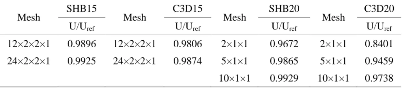
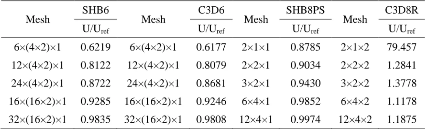
laws...59 Table 3.1. Prismatic, hexahedral and shell finite elements used in the quasi-static analysis..64 Table 3.2. Prismatic, hexahedral and shell finite elements used in the dynamic analysis...65 Table 3.3. Normalized deflection results for the cantilever beam under out-of-plane bending

using linear elements...66 Table 3.4. Normalized deflection results for the cantilever beam under out-of-plane bending

using quadratic elements...66 Table 3.5. Normalized deflection results for the cantilever beam under in-plane bending

using linear elements...67 Table 3.6. Normalized deflection results for the cantilever beam under in-plane bending

using quadratic elements...68 Table 3.7. Normalized deflection results for the cantilever beam under torsion-type loading

using linear elements...69 Table 3.8. Normalized deflection results for the cantilever beam under torsion-type loading

using quadratic elements...69 Table 3.9. Normalized deflection results for the elastic twisted beam under in-plane bending

using linear elements...70 Table 3.10. Normalized deflection results for the elastic twisted beam under in-plane bending

using quadratic elements...70 Table 3.11. Normalized deflection results for the elastic twisted beam under out-of-plane

bending using linear elements...71 Table 3.12. Normalized deflection results for the elastic twisted beam under out-of-plane

bending using quadratic elements...71 Table 3.13. Natural frequency coefficients for the rectangular cantilever plate using linear

elements...72 Table 3.14. Natural frequency coefficients for the rectangular cantilever plate using quadratic

elements...72 Table 3.15. Natural frequency coefficients for the clamped square plate using linear elements

...73 Table 3.16. Natural frequency coefficients for the clamped square plate using quadratic

(13)

- vi -

Table 3.17. Computation details for the pinched semi-cylindrical shell problem...80

Table 3.18. Computation details for the cantilever beam subjected to a concentrated load...84

Table 3.19. Normalized deflection for the cantilever plate with ply dropoffs...94

Table 4.1. Material parameters for the studied 6061-T6 aluminum alloy...102

Table 4.2. Material parameters for the boxbeam...108

Table 4.3. Material parameters for the hemispherical cup...112

Table 4.4. Material parameters for the AA2090-T3 aluminum alloy...116

Table 4.5. Material parameters associated with the anisotropic elastic-plastic model for the cold rolled steel...118

Table 4.6. Material parameters for the aluminum and steel sheets...122

Table 4.7. Springback angles 1 and 2 for the aluminum material...123

Table 4.8. Springback angles ₁ and ₂ for the steel material...124

Table 4.9. Draw-in distances for the aluminum cup at 15 mm punch stroke...126

Table 4.10. Draw-in distances for the steel cup at 40 mm punch stroke...127

(14)

- vii -

List of Figures

Figure 1.1. Commonly used conventional continuum solid elements...7

Figure 1.2. Pure bending of a long beam...8

Figure 1.3. Parasitic bending deformation mode...9

Figure 1.4. Illustration of degenerated shell element...12

Figure 1.5. Geometry of conventional shell elements...13

Figure 1.6. Local coordinate system and nodal variables...14

Figure 1.7. Illustration of a curved beam...16

Figure 1.8. Re-interpolation of the transverse shear strain components by the ANS method ...24

Figure 2.1. Reference geometry and location of integration points for the SHB solid‒shell elements...30

Figure 2.2. Illustration of the local frames used in the formulation of the SHB solid‒shell elements...36

Figure 2.3. Several approaches for computing the element mass matrix...46

Figure 2.4. Traditional linear and substitute piecewise shape functions for a triangular shell element...47

Figure 2.5. 8-node linear hexahedral element...48

Figure 2.6. Schematic representation of the fiber orientations with respect to the local element frame for the SHB20 element...55

Figure 2.7. Illustration of stacking sequence for multilayered composite materials...57

Figure 3.1. Elastic cantilever beam subjected to out-of-plane bending forces...65

Figure 3.2. Elastic cantilever beam subjected to in-plane bending forces...66

Figure 3.3. Elastic cantilever beam subjected to torsion-type forces...67

Figure 3.4. Elastic twisted beam subjected to bending forces...69

Figure 3.5. Simple rectangular cantilever plate as proposed by Anderson et al. (1968)...71

Figure 3.6. Geometry and boundary conditions for the clamped square plate...72

Figure 3.7. Geometry and material parameters for the simply supported square plate...73

Figure 3.8. Loaddisplacement curves for the simply supported square plate...74

Figure 3.9. Geometry and material parameters for the cantilever plate...75

Figure 3.10. Loaddisplacement curves for the cantilever plate under a concentrated force...76

(15)

- viii -

Figure 3.12. Loaddeflection curves for the pinched semi-cylindrical shell...78

Figure 3.13. Geometry and material parameters for the pinched hemispherical shell...80

Figure 3.14. Illustration of the mesh nomenclature for the pinched semi-cylindrical shell...80

Figure 3.15. Loaddisplacement curves for the pinched hemispherical shell...81

Figure 3.16. Geometry and material parameters for the cantilever beam...82

Figure 3.17. Deflection history for the cantilever beam...83

Figure 3.18. Geometry and material parameters for the simply supported elastic beam...84

Figure 3.19. Deflection history for the simply supported elastic beam...85

Figure 3.20. Geometry and material parameters for the clamped circular annular plate...86

Figure 3.21. Deflection history for the clamped circular annular plate...86

Figure 3.22. Geometry and material parameters for the elastic twisted cantilever beam...87

Figure 3.23. Deflection history for the elastic twisted cantilever beam...88

Figure 3.24. Geometry and material parameters for the clamped spherical cap...89

Figure 3.25. Deflection history for the clamped spherical cap...89

Figure 3.26. Geometry and material parameters for the explosively loaded plate...90

Figure 3.27. Deflection history for the explosively loaded plate...91

Figure 3.28. Cantilever plate with ply dropoffs...92

Figure 3.29. Geometry and material parameters for the cantilever laminated beam...94

Figure 3.30. Loaddeflection curves for the cantilever laminated beam...94

Figure 3.31. Undeformed and deformed configurations of the slit laminated annular plate....95

Figure 3.32. Loaddeflection curves for the corner point B for the slit laminated annular plate...95

Figure 3.33. Geometry parameters for the pinched laminated semi-cylindrical shell...96

Figure 3.34. Loaddisplacement curves for the pinched laminated semi-cylindrical shell...97

Figure 3.35. Geometry of the pinched laminated hemispherical shell...97

Figure 3.36. Loaddisplacement curves at points A and B for the pinched laminated hemispherical shell...98

Figure 3.37. Undeformed and final deformed shapes of the pinched laminated hemispherical shell...98

Figure 4.1. Schematic representation of a circular plate subjected to impact by a projectile ...101

Figure 4.2. Initial in-plane mesh for the clamped circular plate under impact by a projectile ...102 Figure 4.3. History of velocity (left) and impact force (right) for the projectile, obtained with the linear SHB elements and ABAQUS shell elements along with the reference

(16)

- ix -

solutions for case 1...103

Figure 4.4. History of velocity (left) and impact force (right) for the projectile, obtained with the linear SHB elements and ABAQUS shell elements along with the reference solutions for case 2...104

Figure 4.5. History of velocity (left) and impact force (right) for the projectile, obtained with the linear SHB elements and ABAQUS solid elements along with the reference solutions for case 1...105

Figure 4.6. History of velocity (left) and impact force (right) for the projectile, obtained with the linear SHB elements and ABAQUS solid elements along with the reference solutions for case 2...106

Figure 4.7. Schematic representation of a boxbeam impacted by an infinite mass...107

Figure 4.8. Coarse and fine undeformed meshes for the boxbeam using the quadratic SHB elements...108

Figure 4.9. Deformed shape for the boxbeam, at time 0.08s, using the linear ABAQUS shell elements...109

Figure 4.10. Deformed shape for the boxbeam, at time 0.08s, using the linear ABAQUS solid elements...109

Figure 4.11. Deformed shape for the boxbeam, at time 0.08s, using the quadratic SHB elements...109

Figure 4.12. Reaction forcedisplacement curves for the impactor using the coarse mesh...110

Figure 4.13. Reaction forcedisplacement curves for the impactor using the fine mesh...110

Figure 4.14. Hemispherical deep drawing setup...112

Figure 4.15. Initial meshes for one quarter of the circular sheet using the linear SHB elements ...112

Figure 4.16. Final deformed shape for the hemispherical cup using the linear SHB elements ...112

Figure 4.17. Simulation results in terms of thickness strain...113

Figure 4.18. Final deformed mesh for the hemispherical cup using ABAQUS C3D8R solid element: illustration of the distorted mesh zone...114

Figure 4.19. Punch force evolution during the deep drawing of the hemispherical cup...114

Figure 4.20. Schematic view for the cylindrical cup drawing process...115

Figure 4.21. Initial meshes for one quarter of the circular sheet...116

Figure 4.22. Final deformed shape for a completely drawn cylindrical cup...116

Figure 4.23. Prediction of cup height profiles...117

Figure 4.24. Schematic view for the rectangular cup drawing setup...118

Figure 4.25. Initial in-plane meshes for a quarter of the rectangular sheet...119

(17)

- x -

Figure 4.27. Prediction of flange contours at different punch strokes for the deep drawing of a

rectangular cup...120

Figure 4.28. Setup of the U-bending tools...121

Figure 4.29. Illustration of the deformed sheet in the U-shape deep drawing test (using SHB20 elements)...121

Figure 4.30. Definition of springback angles ₁ and ₂...122

Figure 4.31. Schematic view for the square cup drawing process...124

Figure 4.32. Final deformed shape for the aluminum square cup at 15 mm punch stroke....124

Figure 4.33. Final deformed shape for the steel square cup at 40 mm punch stroke...124

Figure 4.34. Definition of the drawn-in distances for the final deformed square cup...125

Figure 4.35. Description of the single point incremental forming test...127

Figure 4.36. Final deformed shape for the SPIF sheet...128

Figure 4.37. Simulation results using coarse meshes, in terms of punch force evolution for the SPIF test, along with experiments taken from Bouffioux et al. (2008)...129

Figure 4.38. Simulation results using fine meshes, in terms of punch force evolution for the SPIF test, along with experiments taken from Bouffioux et al. (2008)...130

(18)

(19)

(20)

- 1 -

Introduction

Research background

Nowadays, thin structures are widely employed in many fields of the industry (such as automotive, aerospace, civil engineering) in order to reduce the weight of products and improve their mechanical performances. The finite element (FE) simulation of these thin structures has become an indispensable tool in the design of products and the optimization of manufacturing processes, by replacing a number of expensive and time-consuming experimental tests. Despite the significantly growing development of computational resources, reliability and efficiency of the FE analysis still remain the key features in the simulation practice. Traditionally, for the simulation of thin structures, conventional shell elements are used or alternatively low-order solid elements, when three-dimensional effects need to be accounted for. However, in some circumstances, traditional shell and solid elements suffer from various locking phenomena, such as membrane locking, thickness locking, shear locking, etc. In addition, shell elements are often not appropriate for the modeling of complex problems involving double-sided contact. To remedy these shortcomings, considerable effort has been devoted to the development of more accurate and efficient finite elements during the last few decades.

Membrane finite elements have been widely used, due to their computational efficiency in the simulation of bending as well as stretching-dominated sheet metal forming problems. In order to obtain more accurate results, particular attention has been paid in the literature to the development of shell elements for the modeling of thin structures. Compared to membrane elements, shell elements offer better accuracy for modeling bending effects in thin structures. However, the formulation of classical shell elements is typically based on the assumption of plane-stress conditions, which limits their application in sheet metal forming simulation. Further, they cannot account for thickness variations, since only the mid-plane of the sheet is modeled, which makes the double-sided contact difficult to handle.

Concurrently, continuum solid elements allow more realistic modeling for a number of structural problems thanks to their three-dimensional formulation, thus avoiding geometric (mid-plane) or kinematics assumptions as well as constitutive (plane-stress) restrictions.

(21)

- 2 -

However, in the simulation of thin structures, the use of solid elements involves meshes with too many elements, which is partly attributable to element aspect ratio limitations as well as locking effects in low-order formulations. In addition, several layers of solid elements are required in the thickness direction in order to accurately describe the various nonlinear phenomena, which considerably increases the computational cost of the simulations.

More recently, the concept of solidshell elements has emerged, which represents nowadays an interesting alternative to conventional solid and shell elements, in particular for the simulation of sheet metal forming processes. In fact, solidshell elements combine the advantages of both solid and shell formulations. Their main key features, which make them very attractive, may be summarized as follows: the use of fully three-dimensional constitutive laws, without plane-stress restrictions; easy connection with conventional solid elements, since displacements are the only degrees of freedom; direct calculation of thickness variations, as this is based on physical nodes; automatic consideration of double-sided contact; ability to accurately model thin structures with only a single element layer and few integration points in the thickness direction.

The current work contributes to the development of a family of assumed strain based solidshell elements (SHB) for the three-dimensional modeling of thin structures. These formulations are extended to include geometric and material nonlinearities, following the earlier works on the family of SHB elements. The first solid–shell element in this family was developed by Abed-Meraim and Combescure (2002), and consists of an eight-node hexahedral element denoted SHB8PS. Its formulation was subsequently improved by Abed-Meraim and Combescure (2009), especially in terms of locking reduction, while the hourglass modes were efficiently controlled by implementing a new stabilization procedure. Then, a six-node prismatic solid–shell element denoted SHB6 was developed by Trinh et al. (2011), as a complement to the SHB8PS element for the modeling of complex geometries whose meshing requires the combination of hexahedral and prismatic elements. Although the performance of the SHB6 is good on the whole, its convergence rate remains slower than that of the SHB8PS, and it requires finer meshes to obtain accurate solutions. More recently, the quadratic counterparts of the above hexahedral and prismatic solid–shell elements have been developed by Abed-Meraim et al. (2013), in order to improve the overall performance and convergence rate. These quadratic versions consist of a 20-node hexahedral element, denoted SHB20, and

(22)

- 3 -

a 15-node prismatic element, denoted SHB15. Likewise, their formulation is based on a fully three-dimensional approach with an in-plane reduced-integration rule.

Objectives of the thesis

In this work, a family of SHB solid‒shell elements, which includes linear prismatic and hexahedral solid‒shell elements, and their quadratic counterparts, is developed for the three-dimensional modeling of thin structures. With respect to the earlier contributions of Abed-Meraim and co-workers on the SHB family elements, we summarize hereafter the main objectives of the current work:

- The SHB elements proposed in this contribution represent extensions of the previous quasi-static versions. They are formulated here with a new lumped mass matrix, in order to deal with explicit/dynamic problems and complex sheet metal forming simulations;

- In the current contribution, the formulation of the SHB elements is combined with various types of constitutive equations, including classical isotropic elastic behavior, orthotropic elastic behavior for composite materials, and anisotropic plastic behavior for metallic materials;

- In this work, all SHB elements have been implemented into the ABAQUS static/implicit and dynamic/explicit software packages, in order to extend their application range to nonlinear quasi-static and dynamic analyses;

- In contrast to previous contributions, which were restricted to academic benchmark problems, the range of application of the proposed SHB elements is enlarged in the current work to include selective dynamic and impact-type problems as well as challenging sheet metal forming processes, involving complex (nonlinear) strain paths, large-strain anisotropic plasticity and double-sided contact.

Organization of the thesis

The thesis manuscript is structured into four main chapters, which are described as follows. The first chapter introduces a literature review on the state-of-the-art of finite element technologies used for the modeling of thin structures. Then, a unified formulation for the

(23)

- 4 -

proposed four solid‒shell elements is presented in Chapter 2. In Chapter 3, various popular benchmark tests are conducted in order to assess the performance of the SHB elements in quasi-static and dynamic analyses. To further evaluate the performance of the SHB elements in complex highly nonlinear test problems, the proposed solid‒shell elements are applied in Chapter 4 to the simulation of impact-type problems as well as challenging sheet metal forming processes, involving geometric nonlinearities, anisotropic elasto-plastic behavior, and double-sided contact. Finally, the main conclusions and remarks on the current contribution as well as some prospects for future work are drawn in the conclusion part of this manuscript.

(24)

- 5 -

Chapter 1 Literature review on solid‒shell finite

element technology

Introduction

In order to save materials, reduce their weight and improve the whole mechanical performance, thin structures are nowadays increasingly used in modern industries. The rapid development of computational resources has made the finite element (FE) analysis of thin structures possible in the design and manufacturing processes. However, the reliability and accuracy of the predicted solutions still remain to be improved.

It is well known that shell theory allows developing highly efficient finite elements; in particular, through their degenerated formulations. In this regard, conventional shell elements have been most often adopted for the FE analysis of thin structures. Although shell elements involve relatively low computational costs, their degenerated formulations lead to several limitations. For instance, the formulation of classical shell elements is typically based on the assumption of plane-stress conditions, which limits their application in sheet metal forming simulation. Further, they cannot account for thickness variations, since only the mid-plane of the sheet is modeled, which makes the double-sided contact difficult to handle. Moreover, shell elements also suffer from various locking phenomena, in particular in the simulation of bending-dominated problems. Concurrently, solid elements have been developed based on fully three-dimensional formulations, which allow physical modeling of thickness variations. However, locking phenomena are also present in these conventional solid elements, in particular for low-order formulations, which cannot be avoided by just refining the mesh.

To remedy these shortcomings, considerable effort has been devoted to the development of solid‒shell elements during the past few decades. The key idea behind this original concept of solid‒shell elements is to combine the advantages of both solid and shell formulations. The main benefits of the resulting solid‒shell concept may be summarized as follows: easier

(25)

- 6 -

formulation, based on a purely three-dimensional approach, with displacements as the only degrees of freedom; consideration of fully three-dimensional constitutive laws, without plane-stress restrictions; direct calculation of thickness variations; natural treatment of double-sided contact, thanks to the availability of actual top and bottom surfaces; 3D modeling of thin structures, using only a single element layer and few integration points, while accurately describing the through-thickness phenomena.

In this chapter, a literature review on the development and the use of FE technologies for the simulation of thin structures is presented. The remaining sections of this chapter are organized as follows. In a short introduction, the conventional solid and shell formulations are summarized in Subsections 1.1 and 1.2, respectively. Then, the concept of solid‒shell elements and related numerical techniques are introduced in Subsection 1.3. The last Subsection is dedicated to the state-of-the-art of the solid–shell elements whose formulation will be further developed and extended in the current work.

1.1 Three-dimensional solid finite elements

1.1.1 State of the art

Continuum solid finite elements are usually used to model three-dimensional bulk structures without any geometric simplifications. The geometry of continuum solid elements is completely defined by the coordinates of the nodes, and the nodal displacements allow the interpolation of the displacements within the element in all directions. Moreover, fully 3D constitutive equations are adopted for these solid elements, which allow a realistic description of the various phenomena without the need for restrictive assumptions (e.g., plane-stress conditions). Nowadays, the most commonly used continuum elements in finite element analysis are the tetrahedral elements, prismatic elements and hexahedral elements, as illustrated in Fig. 1.1 (see, e.g., Hellen, 1972; Andersen, 1979; Hughes, 1987; Zienkiewicz and Taylor, 2000; Cao et al., 2002). These elements usually have four, six and eight nodes, respectively, in the case of linear element formulations, while they have ten, fifteen and twenty, respectively, in the case of quadratic element formulations. Generally, it is well known that the order hexahedral elements provide more accurate solutions than the low-order tetrahedral and prismatic elements for most nonlinear problems (see, e.g., Puso and Solberg, 2006). However, hexahedral elements are not suitable to mesh complex geometries

(26)

- 7 -

and, in such situations, tetrahedral or prismatic elements are useful. Also, the high-order tetrahedral and prismatic elements can be used to model nonlinear problems involving complex geometries, however, at the expense of a higher computational cost.

4-node tetrahedron

10-node tetrahedron

6-node triangular prism

15-node triangular prism

8-node hexahedron

20-node hexahedron

Figure 1.1. Commonly used conventional continuum solid elements. 1.1.2 Treatment of locking phenomena

As mentioned above, solid elements have many advantages, due to their fully three-dimensional formulations, and are designed to be general-purpose elements. In most nonlinear situations, the low-order solid elements are preferred due to their lower computational cost. However, they often show poor performance and suffer from several locking phenomena in simulations of thin structures, especially for bending-dominated problems (see, e.g., Adam et al., 2014, 2015a). These locking phenomena, which significantly compromise the performance of solid elements, are briefly presented in what follows.

1.1.2.1 Shear locking

The shear locking usually occurs when the elements are subjected to bending-dominated forces or moments. This shear locking is due to the fact that the finite element is not able to model pure bending situations without introducing (spurious) transverse shear strains, which results in excessive element stiffness in shear (see, e.g., Prathap, 1985; Huang, 1987; Tessler and Spiridigliozzi, 1988). Regarding this point, the following example illustrates the case of a long beam with rectangular cross section subjected to pure bending moment, as shown in Fig. 1.2.

(27)

- 8 -

M

x

y

2L

b

2t

Figure 1.2. Pure bending of a long beam.

Theoretically, the analytical solution of this in-plane beam bending problem is given by the following expressions:



2 2





2 2



M M M , L t , I 2 I 2 I u xy v x y E E E       (1.1)

where u and v are the displacements in the x and y directions, respectively. The geometric dimensions 2t, b and 2L represent the thickness, the width and the length of the beam. The elastic properties are given by E for the Young modulus, and  for the Poisson ratio. Also, in the above formulas, I denotes the inertia moment of the beam section, while M is the bending moment.

The strain components are derived from the above in-plane displacements as follows:

M M , , 0. I I x y xy u v u v y y x E y E y x                (1.2)

From the above expressions, it is clear that the shear strain xy satisfies the

zero-shear-strain condition, which is consistent with a beam in pure bending.

From a finite element point of view, the displacement field can be interpolated using the following classical functions:

,            xy b y b x b b v xy a y a x a a u 3 2 1 0 3 2 1 0 (1.3)

where the eight coefficients a and _i b represent the eight deformation modes, as illustrated in _i Table 1.1.

(28)

- 9 -

Table 1.1. Deformation modes for beam problems.

Coefficient a0 0 a1 0 a2 0 a3 0

Mode

Coefficient b0 0 b1 0 b2 0 b3 0

Mode

Considering the pure bending condition, only the fourth mode (a₃ 0) is active. Thus, the interpolations given in Eq. (1.3) degenerate to

.      0 3 v xy a u (1.4)

The strain components associated with the above displacement field are given by . , 0 , ₃ 3 a x x v y u y v y a x u xy y x                   (1.5)

The above expressions clearly show that the resulting strain components do not satisfy the zero-shear-strain condition of pure bending, which leads to a stiffer element, and thereby to a parasitic deformation mode, as shown in Fig. 1.3 (see, e.g., Belytschko and Bindeman, 1993; Li and Cescotto, 1997). M M x y 2L b 2t

(29)

- 10 -

The parasitic shear strain that appears in Eq. (1.5) is represents the shear locking, which is well known in finite element analysis. This phenomenon appears especially for low-order finite elements, due to their particularly simple kinematics, which is not rich enough to represent the correct solution. The shear locking phenomenon can be prevented by using specific numerical treatments, such as the reduced-integration technique (see, e.g., Zienkiewicz et al., 1971), the assumed-strain method (see, e.g., Belytschko and Bindeman, 1993), or possibly the consideration of higher-order elements.

1.1.2.2 Poisson thickness locking

The Poisson thickness locking may also occur in low-order hexahedral elements. To illustrate this phenomenon, let us consider again the pure bending problem described above. According to the displacement interpolation given by Eq. (1.3), the strain components in the

x and y directions can be obtained as:

1 3 2 3 . x y u a a y x v b b x y         _   _  _ _{ }   (1.6)

Based on the elastic strainstress relationship, the corresponding stress components are given by









,          y x y x y x           2 2 (1.7) where











  2 1 1   E and







   1 2 E .

It can be noticed that a constant approximation for the thickness strain y is obtained,

while the corresponding stress y has a linear distribution along the y



direction (for  0). Such inconsistency between the distribution of the stress and the strain in the thickness direction leads to the undesirable locking effect, denoted as the Poisson thickness locking. The latter can be alleviated by modifying the elastic constitutive matrix so that the normal stress is uniformly distributed through the thickness (see, e.g., Petchsasithon and Gosling, 2005).

(30)

- 11 -

1.1.2.3 Volumetric locking

When incompressible or nearly-incompressible material behavior is considered, standard fully integrated finite elements usually suffer from the so-called volumetric locking phenomenon. The latter cannot be avoided just by refining the mesh and, thus, some finite elements show poor performance when the Poisson ratio approaches the limit value of 0.5. To better illustrate this locking effect, we consider here a linear elastic material. The elastic strain can be decomposed into a deviatoric part ε and a volumetric part _d ε_v tr

 

ε . Consequently, the elastic strain energy _int of the involved element is also partitioned into a deviatoric (distortional) part dev and a volumetric part v as follows:

 



           e e e e d tr K d G _d _d 2 v dev int 2 ε :ε ε , (1.8) where

_

_

   1 2 E

G is the shear modulus, and

_

_



2 1

3 

 E

Κ is the bulk modulus.

For incompressible or nearly-incompressible materials, the bulk modulus K will become extremely large when the Poisson ratio  approaches the limit value of 0.5. Consequently, the associated element becomes overly stiff, as compared to that of real incompressible materials, if _ii tr

 

 is not vanishing (see Nguyen, 2009). Generally, the selective reduced integration rule, the Galerkin mixed formulation and stabilization techniques may be used to alleviate this type of locking (see, e.g., Elguedj et al., 2008; Davim, 2012). In some cases, the volumetric locking can also be prevented by defining nodal volumes and by evaluating average nodal pressures in terms of these designed local volumes instead of using the whole element volume (Bonet and Burton, 1998).

1.2 Conventional shell elements

Conventional shell elements have been specifically developed for the analysis of thin structures (i.e., when the thickness dimension is significantly smaller than the other dimensions). According to the theoretical backgrounds on which their formulations are based, shell elements can be classified into two main families: the conventional flat shells and the degenerated shells. For the conventional flat shell elements, the geometry of the shell is

(31)

- 12 -

approximated by a flat finite element. Some classical theories, such as the Kirchhoff theory for thin plates and the Reissner‒Mindlin theory for thick plates, are generally adopted as basic theoretical models for the formulation of flat shell elements, which is well detailed in several finite element books (see, e.g., Bathe, 1996; Zienkiewicz and Taylor, 2000). For the second family of shell elements, the latter are degenerated from the formulation of three-dimensional finite elements, and commonly used to represent the mid-surface of thin structures, as illustrated in Fig. 1.4 for a 4-node shell element. In most shell theories, some basic assumptions are essentially made for the purpose of implementation. In general, the following assumptions are widely considered in shell element formulations:

 The consistent physical thickness of the simulated structure is neglected.

 The normal to the mid-surface remains straight after deformation.

 The transverse normal stress is assumed negligible.

z

x

y

o

x'

y'

z'

shell mid-surface

Figure 1.4. Illustration of degenerated shell element.

Neglecting the physical thickness, the plane-stress conditions are adopted in the formulation of shell elements, which allows improving the computational efficiency. Therefore, shell elements usually perform more efficiently than continuum solid elements. According to their geometric characteristics, four commonly used shell elements, including linear triangular and quadrilateral shell elements, and their quadratic counterparts, have been developed in the literature (see the illustrative Fig. 1.5).

(32)

- 13 -

3-node triangular element 4-node quadrilateral element

6-node triangular element 8-node quadrilateral element

Figure 1.5. Geometry of conventional shell elements.

The widely used degenerated shell elements are derived from the pioneering work of Ahmad et al. (Ahmad et al., 1970), who developed a curved shell element for thick and thin structures. In what follows, only some basic concepts of degenerated shell elements are briefly introduced in order to subsequently compare their main features with those of solid‒shell elements.

1) Geometry and kinematic interpolation

As mentioned above, the degenerated shell elements are obtained from the reduction (degeneration) of the 3D solid approach to the 2D shell approach, which has only mid-surface nodal variables. As illustrated in Fig. 1.6, a local orthogonal coordinate system (V₁_i,V₂_i,V₃_i) associated with the shell element is defined, in which the unit vector V represents the 3i

direction normal to the mid-surface. The nodal coordinates (x,y,z) and nodal displacements (u,v,w) at the i-th node of the shell element can be interpolated using the three translational displacements (u,v,w) and the two rotations (, ) at the two points i_top and i_bottom. The detailed equations are well explained in some well-established references (see, e.g., Ahmad et al., 1970; Choi and Paik, 1995; Polit and Touratier, 1999; Zienkiewicz and Taylor, 2000).

(33)

- 14 -

z

x

y

o

x'

y'

z'

i

_top

i

_bot

α

_i

β

_i i 3

V

i 2

V

i 1

V

Figure 1.6. Local coordinate system and nodal variables (Ahmad et al., 1970). 2) Definition of the strain and stress fields

In the local coordinate system (x ,'y ,'z'), the strain field is derived from the expression of the displacement gradient, while the stress field is computed by the constitutive equations associated with the shell element. According to the classical shell assumptions, the stress in the thickness direction is assumed to be negligible. Hence, the strain field corresponding to the plane-stress conditions is expressed as:

 

ˆ ' ', ' ', 2 ' ', 2 ' ', 2 ' ' , T x x y y x y y z z x          _{ } _ ε u (1.9)

where vector uˆ is the displacement field within the shell element, which is interpolated using the nodal displacements u



u,v,w



. The corresponding stress field is given by:

' ', ' ', ' ', ' ', ' ' . T x x y y x y y z z x           σ (1.10)

Then, the elastic stressstrain relationship is written as:

e

 

σ C , (1.11)

(34)

- 15 -













, 2 1 0 2 1 0 0 2 1 0 0 0 1 0 0 0 1 1 2                           k sym k E e C (1.12)

where the shear correction factor k5 6 is introduced to account for the parabolic shear stress distribution across the section (see, e.g., Vlachoutsis, 1992).

3) Variational principle

Finally, the variational form of the virtual work expression for the conventional shell elements writes:

 





int ˆ 0, e T _T ext e W W d           

_

 u σ   u R  (1.13)

where vector R represents the equivalent external nodal force vector. 1.2.2 Locking phenomena

For the last decades, conventional shell elements have attracted much attention for the analysis of thin structures, due to their high efficiency. However, a number of locking phenomena also exist in conventional shell elements, which are especially revealed in the simulation of thin structures. In this subsection, two typical locking phenomena, i.e. the transverse shear locking and the membrane locking, which are commonly identified in conventional shell elements, are briefly presented.

1.2.2.1 Transverse shear locking

Similar to the solid elements discussed previously, the transverse shear locking is one of the most commonly encountered locking phenomena in shell elements. This locking is due to the fact that the Kirchhoff‒Love hypothesis is not considered in the displacement interpolations, which does not allow reproducing the zero-transverse-shear-strain condition in pure bending problems (see, e.g., Zienkiewicz et al., 1971; Kui et al., 1985; César de Sá et al., 2002). The illustration of the specific mechanism leading to the occurrence of transverse shear locking, in relation with the resulting parasitic shear strain, is similar to what has been shown in subsection 1.1.2.1, and is not repeated here for conciseness.

(35)

- 16 -

1.2.2.2 Membrane locking

The membrane locking is characterized by the occurrence of parasitic membrane strains in bending-dominated problems of curved beam and shell structures. This locking phenomenon is a severe issue, which is frequently encountered in both low-order and high-order shell elements (see, e.g., Stolarski and Belytschko, 1982; Koschnick et al., 2005; Nguyen, 2009). In order to clearly explain the origin of membrane locking, we present here a simple curved beam with length L and radius R, as illustrated in Fig. 1.7. Based on the classical thin beam theory (see, e.g., Timoshenko, 1955), the displacement degrees of freedom are defined as the circumferential displacement u and the radial displacement w . The coordinate s is aligned so that to follow the middle line of the curved beam.

F

s

Figure 1.7. Illustration of a curved beam.

With these definitions, the membrane strain  and the bending strain  are derived from the displacement field as follows:

, , , R R s s ss u w u w          . (1.14)

From the above expressions, it is clearly suggested that interpolations of class C0 and C2 are required for the displacements u and w , respectively, which leads to the following expressions: ,          3 3 2 2 1 0 1 0     b b b b w a a u (1.15)

where  s L, and coefficients a and _i b_j (i0,1 and j0 to 3) are expressed in terms of the nodal degrees of freedom.

(36)

- 17 -

According to the expressions given in Eq. (1.15), the membrane strain  and the bending strain  can be rewritten as:



 









 



.                  2 3 2 2 1 3 3 2 2 1 0 1 L 6 L 2 RL R R R R L b b a b b b b a (1.16)

Considering the physical response of inextensional bending, which is usually the case for curved beams and shells, it is required that the membrane strain  tends to vanish. In this case, the following constraints must to be satisfied:

.            0 R 0 R 0 R 0 R L 3 2 1 0 1 b b b b a (1.17)

In the above system of equations, including the terms from both the circumferential and radial displacements, the first expression represents the true constraint and it reflects the physical condition of curved beams, for which the membrane strain  0. However, the remaining three constrains, b₁0, b₂ 0 and b₃0, involve the following spurious constraints: w,s 0, w,ss0 and w,sss0, which will excessively increase the bending

stiffness of the element and cause the so-called membrane locking (see Nguyen, 2009). 1.2.3 Numerical methods for alleviating locking problems

Locking phenomena usually occur when low-order fully integrated elements are adopted in the simulations. Therefore, the stiffness of the investigated element is overestimated due to non-physical (spurious) deformations. A number of methods and techniques have been developed in the literature to overcome these locking phenomena for both solid and shell elements. The reduced integration (RI) technique was the first numerical method to alleviate some locking phenomena (see, e.g., Hughes et al., 1978; Stolarski and Belytschko, 1982, 1983; Briassoulis, 1989; Belytschko et al., 1992; Zhu and Cescotto, 1996; Hauptmann et al., 2000; Geyer and Groenwold, 2003; Parente et al., 2006; Schwarze and Reese, 2009; Winkler, 2010; Schwarze et al., 2011; Bouclier et al., 2012; Edem and Gosling, 2013; Pagani et al., 2014). However, not all locking phenomena can be alleviated by the RI technique, which requires additional treatments to improve the performance of shell elements (see, e.g., Zienkiewicz et al., 1971; Hughes et al., 1978).

(37)

- 18 -

The most effective solution to prevent the occurrence of locking problems is the use of mixed formulations, in which separate (independent) interpolations are adopted for the displacements and the stresses, or by the projection of the nodal displacements so that the spurious deformations are minimized (see, e.g., Rhiu and Lee, 1987; Chang et al., 1989; Polit and Touratier, 2000; Brischetto et al., 2012). In this context, the so-called assumed strain method (ASM) has been introduced for shell elements by Bathe and Dvorkin (1986), and was extensively applied to solid elements (see, e.g., Belytschko and Bindeman, 1993; Zhu and Cescotto, 1996; Flores, 2013a). By combining the ASM with the RI technique, the resulting elements showed good performances with respect to shear and volumetric locking phenomena. The enhanced assumed strain (EAS) technique is also widely used in the formulation of low-order finite elements, which is based on the inclusion of additional deformation modes for removing locking problems (see, e.g., Simo and Rifai, 1990; Simo and Armero, 1992). The EAS technique is often combined with the assumed natural strain (ANS) method in order to prevent most locking phenomena (see, e.g., Wagner et al., 2002). The numerical techniques discussed above have been widely applied in the literature for 2D and 3D solid and shell element formulations, which ultimately motivated the efficient and accurate concept of solidshell elements for the 3D modeling of thin structures.

1.3 Solid–shell finite elements

During the past few decades, the concept of ―solid‒shell‖ elements has attracted significant attention from researchers and FE developers. The main objective of developing solid–shell elements is to allow three-dimensional modeling of thin structures, without the occurrence of locking effects, while accounting for the through-thickness phenomena. In other words, solid– shell elements are aimed to combine the advantages of both conventional shell elements and continuum solid formulations. A general comparison, in terms of advantages and drawbacks, for conventional shell elements, solid elements and solid–shell elements is proposed in Table 1.2.

(38)

- 19 -

Table 1.2. Comparison between different FE technologies.

Shell elements Solid elements Solid‒shell elements

Advantages

 only the mid-plane is discretized  low computational cost  Direct modeling of thickness  fully 3D constitutive equations

 Direct modeling of thickness.  fully 3D constitutive equations  only displacement DOF

 locking-free

 low computational cost (only a single layer of elements)

Disadvantages  plane-stress assumptions  locking problems  high computational cost  locking problems

As mentioned in the above Table, the main benefits of the solid‒shell concept can be summarized as follows: direct calculation of thickness variations thanks to the three-dimensional formulation, with displacements as the only degrees of freedom; consideration of fully three-dimensional constitutive laws, with no plane-stress restrictions; natural treatment of double-sided contact, which makes them more suitable for industrial applications; 3D modeling of thin structures with only a single element layer and few integration points, while accurately describing the through-thickness phenomena.

Several numerical techniques have been developed for solid‒shell elements to alleviate most locking pathologies. Among them, the reduced integration (RI) technique (see, e.g., Zienkiewicz et al., 1971) or the selective reduced integration (SRI) technique (see, e.g., Hughes, 1980), which consists, for low-order solid‒shell elements, in adopting a one-point in-plane quadrature rule, while considering several integration points along the thickness. Such RI techniques make the solid‒shell elements very attractive in terms of computational cost, since they only require few integration points in the simulations. However, due to the low quadrature order, some elements may be subjected to spurious zero-energy modes (hourglass modes), which require specific procedures for their stabilization (see, e.g., Abed-Meraim and Combescure, 2009). Furthermore, several additional strategies have been combined with the

(39)

- 20 -

above techniques in order to improve the performance of solidshell elements with regard to locking effects. The most widely used are the assumed strain method (ASM), the enhanced assumed strain (EAS) approach, and the assumed natural strain (ANS) concept (see, e.g., Cho et al., 1998; Hauptmann and Schweizerhof, 1998; Puso, 2000; Sze and Yao, 2000; Abed-Meraim and Combescure, 2002; Alves de Sousa et al., 2005; Parente et al., 2006; Reese, 2007; Cardoso et al., 2008; Abed-Meraim and Combescure, 2009; Schwarze and Reese, 2009; Moreira et al., 2010; Li et al., 2011; Edem and Gosling, 2012; Bouclier et al., 2013a, 2013b; Flores, 2013a, 2013b; Naceur et al., 2013; Pagani et al., 2014; Bouclier et al., 2015; Caseiro et al., 2015; Ben Bettaieb et al., 2015; Kpeky et al., 2015; Flores, 2016).

1.3.2 Treatment of locking phenomena

In order to eliminate the locking phenomena and to improve the overall performance, several numerical treatments are commonly adopted in the formulation of solid‒shell elements. In this subsection, we briefly present the four most commonly used methods for solid‒shell elements, which consist of the ASM, the EAS, the ANS, the mixed method and the NURBS-based formulation.

1.3.2.1 Assumed strain method (ASM)

Based on the variational framework, the so-called assumed strain method is frequently adopted in the formulation of solidshell elements. In the pioneering works of Hughes (1980), the ― B -bar approach‖ has been introduced in order to specifically solve volumetric locking problems. This approach consists of the projection of the classical discrete gradient operator B into an assumed (projected) gradient operator B , in which the contribution of the volumetric part is reduced (see also Simo and Hughes, 1986). Later on, a number of contributions have proved that the ASM method is able to significantly enhance the performance of finite elements, including solidshell elements (see, e.g., Belytschko and Bindeman, 1991, 1993; Stolarski and Chen, 1995; Li and Cescotto, 1997; Cho et al., 1998; Abed-Meraim and Combescure, 2002; Hong and Kim, 2002; Lee et al., 2002; Flores and Oñate, 2005; Kulikov and Plotnikova, 2006; Abed-Meraim and Combescure, 2009; Wisniewski et al., 2010).

The assumed strain method (ASM) is usually based on the well-known Hu‒Washizu three-field variational principle (see, e.g., Simo et al., 1985; Simo and Hughes, 1986; Belytschko and Bindeman, 1991, 1993). The weak form of the Hu‒Washizu principle is expressed by

(40)

- 21 -





T T



 



T ext s , , d d 0, e e e e        v ε σ 



ε σ   



σ   v ε   d f  (1.18) where  denotes a variation, v the velocity field, ε the assumed strain rate, σ the interpolated stress, σ the stress evaluated by the constitutive law, d the nodal velocities, fext

the external nodal forces, and _s

 

v the symmetric part of the velocity gradient.

As suggested by Simo and Hughes (1986), the interpolated stress σ is assumed to be orthogonal to the difference between the symmetric part of the velocity gradient _s

 

v and the assumed strain rate ε , which leads to the following simplified form of the Hu‒Washizu variational principle

 

T T ext d 0. e e      ε 



ε σ    d f  (1.19)

The symmetric part of the velocity gradient s

 

v is related to the nodal velocities d by using the classical discrete gradient operator B as follows



( ) ( )



( ) ( ), ) , ( 1 s s x t N x t x t n I I d B d v      



(1.20)

where N represent the shape functions, and _I I 1, ,n , with n being the number of element nodes.

The assumed strain rate ε is expressed in terms of a modified matrix B , which is derived from the classical gradient operator B , in order to eliminate most locking phenomena. Its expression is given by ). ( ) ( ) ( ) ( ) , (x t x _I t x t n I d B d B ε 



   1 (1.21) Substituting Eq. (1.21) into the simplified form of the Hu‒Washizu variational principle (see Eq. (1.19)), we obtain:





T T ext d 0. e e   

_

    d B σ f (1.22)

Since d can be chosen quite arbitrarily, Eq. (1.22) leads to the following expressions of the element stiffness matrix and internal force vector:

T ep int T

d , ( ) d

e e

e 



_   e 



_  e

K B C B f B σ ε , (1.23)

(41)

- 22 -

1.3.2.2 Enhanced assumed strain (EAS) method

The enhanced assumed strain method (EAS) proposed by Simo and Rifai (Simo and Rifai, 1990) also attracted much interest for overcoming the locking deficiencies over the past two decades (see, e.g., Simo and Rifai, 1990; Puso, 2000; César de Sá et al., 2002; Areias et al., 2003; Bui et al., 2004; Pimpinelli, 2004; Valente et al., 2004; Cardoso et al., 2008; Nguyen, 2009; Li et al., 2011; Sena et al., 2011; Flores, 2013b, Ben Bettaieb et al., 2015).

The fundamental principle of the EAS method consists in the addition of an extra enhanced assumed strain field E~ to the displacement-based strain field Ecom (also known as the compatible strain field), which leads to the following improved strain field E :

com 

 

E E E . (1.24)

Substituting the modified strain field into the Hu‒Washizu variational principle, the latter writes:



, ,



int



, ,



ext

 

,

 u E S   u E S   u (1.25)

where the internal and external potentials are given by:





 

e int ext _S , , d : d , d dS e e e e e e e W                   



u E S E S E u u b u t  (1.26)

where u is the displacement field, E is the enhanced strain field and S is the stress field.

 

E

W denotes the strain energy, while b and t represent the body forces and the traction forces, respectively.

As suggested by Simo and Rifai (1990), the stress field S is eliminated from the above equation via the following orthogonality condition:

: d 0

e e



  



S E , (1.27)

which is analogous to that considered by Simo and Hughes (1986) for the ASM approach. Accordingly, the first variation of Eq. (1.25) writes:









 



~



:

 

. , , , ,



 _                e e e e e W e S com ext int dS d d u b u t E E E E u S E u S E u          (1.28)

(42)

- 23 -

The linearization of the above simplified form of the Hu‒Washizu variational principle leads to the following system of equilibrium equations:

ext , uu u u u                  _{ } _       d K K f f α K K f (1.29)

where d denotes the nodal displacements, and α the enhancing parameters. The matrices involved in Eq. (1.29) include the classical displacement-based stiffness matrix K , the uu enhanced stiffness operator K, and the coupling stiffness matrices Ku and Ku . The internal forces u

f and f are associated with the displacement field and the enhanced field,  respectively.

By solving the above equilibrium equations, the final condensed element stiffness matrix

e

K can be obtained as:

 

1 . uu u u e         K K K K K (1.30)

1.3.2.3 Assumed natural strain (ANS) method

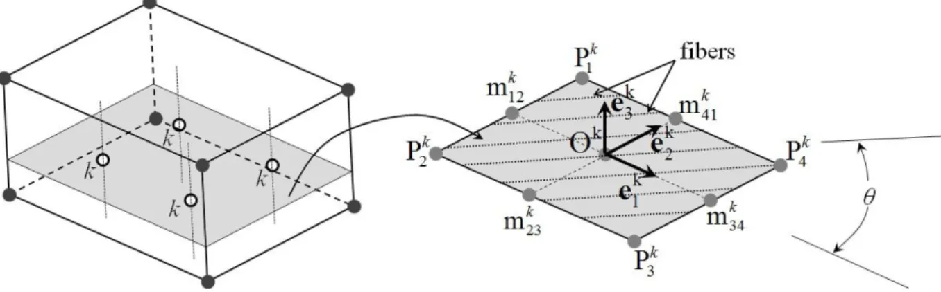
The ANS method consists in interpolating the shear strains at specific locations instead of using the standard displacement-based strain field, which allows significantly reducing the shear and volumetric locking. Such interpolation, also known as the mixed-interpolation method, can be traced back to the work of Hughes and Tezduyar (1981) for Mindlin plates, and later extended to shell elements by Dvorkin and Bathe (1984). The ANS method has been widely applied for the improvement of various finite elements (see, e.g., Bathe and Dvorkin, 1986; Militello and Felippa, 1990a, 1990b; Hauptmann and Schweizerhof, 1998; Sze and Zhu, 1999; Sze and Yao, 2000; Sze and Chan, 2001; Kim and Kim, 2002; Vu-Quoc and Tan, 2003; Lee, 2004; Kim et al., 2005; Klinkel et al., 2006; Cardoso et al., 2008; Schwarze and Reese, 2009; Nguyen, 2009; Norachan et al., 2012; Edem and Gosling, 2012, 2013; Flores, 2013b; Caseiro et al., 2014, 2015).

In order to describe the basic concept of the ANS method, an isoparametric 8-node hexahedral solid‒shell element is considered here, as illustrated in Fig. 1.8. It is well known that, for solid‒shell elements, only displacements are taken as degrees of freedom and, thus, the local strain field Eloc can be related to the nodal displacements dloc by the discrete gradient operator B as follows:

Éléments finis solide-coque pour l’analyse quasi-statique et dynamique des structures minces 3d : application aux procédés de mise en forme

HAL Id: tel-01540345

https://pastel.archives-ouvertes.fr/tel-01540345

et dynamique des structures minces 3d : application aux

procédés de mise en forme

Peng Wang

To cite this version:

Peng WANG

Solid



shell finite elements for quasi-static and

dynamic analysis of 3D thin structures:

Application to sheet metal forming processes

Doctorat ParisTech

T H È S E

l’École Nationale Supérieure d'Arts et Métiers

Spécialité “ Mécanique - matériaux ”

T

H

È

S

E

To my beloved parents for their sacrifices

To my beloved sisters and brothers for their support

To my dear supervisors for their guidance

To all my dear friends for their help

Acknowledgments

Contents

List of Tables

List of Figures

Introduction

Research background

Objectives of the thesis

Organization of the thesis

Chapter 1

Literature review on solid‒shell finite

element technology

Introduction

1.1 Three-dimensional solid finite elements

M

M

x

y

2L

b

2t



























 

 













 

1.2 Conventional shell elements

z

x

y

o

x'

y'

z'

shell mid-surface

z

x

y

_

_

_

_

_

_