HAL Id: hal-01717324
https://hal.archives-ouvertes.fr/hal-01717324
Submitted on 6 Nov 2019
HAL is a multi-disciplinary open access
archive for the deposit and dissemination of
sci-entific research documents, whether they are
pub-lished or not. The documents may come from
teaching and research institutions in France or
abroad, or from public or private research centers.
L’archive ouverte pluridisciplinaire HAL, est
destinée au dépôt et à la diffusion de documents
scientifiques de niveau recherche, publiés ou non,
émanant des établissements d’enseignement et de
recherche français ou étrangers, des laboratoires
publics ou privés.
Temperature correction of radiometric and geometric
models for an uncooled CCD camera in the near infrared
Thierry Sentenac, Yannick Le Maoult, G Rolland, M Devy
To cite this version:
Thierry Sentenac, Yannick Le Maoult, G Rolland, M Devy. Temperature correction of radiometric
and geometric models for an uncooled CCD camera in the near infrared. IEEE Transactions on
Instrumentation and Measurement, Institute of Electrical and Electronics Engineers, 2003, 52 (1),
pp.46-60. �10.1109/TIM.2003.809103�. �hal-01717324�
Temperature Correction of Radiometric
and Geometric Models for an Uncooled
CCD Camera in the Near Infrared
Thierry Sentenac, Yannick Le Maoult, Guy Rolland, and Michel Devy
Abstract—This paper presents radiometric and geometric
models for both temperature and displacement noncontact mea-surements using an uncooled charge-coupled device (CCD) video camera. Such techniques (“one sensor-two measures”) represent an interest in many industrial low cost applications and scientific domains.
To benefit from both measurements, we have to use the camera’s spectral response in the near infrared spectral band from 0.75 to 1.1 m. In this spectral band, the temperature variations of an uncooled CCD camera are taken into account in the radiometric and geometric models. By using physical models for CCD camera, we quantify detector’s quantum efficiency, sensor noise and spa-tial resolution as a function of the wavelength and of the detector temperature. These models are confirmed by experimental results of calibration with a low cost uncooled camera based on a Sony de-tector and operating over the dede-tector temperature range of -30 to –50 .
Index Terms—Camera calibration, charge-coupled device
(CCD) cameras, geometric model, modulation transfer function (MTF), noise estimation, radiometric model, sensor modeling, spatial resolution, temperature.
I. INTRODUCTION
I
N RECENT YEARS, the material research center of the Ecole des Mines d’Albi-Carmaux (CROMeP) has developed temperature gradient measurements based on infrared thermo-graphic cameras [1]. At the same time, a team has been involved in three-dimensional (3-D) deformation [2] and distortion [3] measurements using charge-coupled device (CCD) cameras. To improve maintenance and cost in industrial applications, we have to measure both temperature and dimensional characteris-tics using only one noncontact sensor. The system must be able to measure a temperature from 350 to 1000 C with a tolerance of 25 C and spatial surface deformations of 0.1 mm with an observation distance of 1 m.However, the main difficulty is the temperature measurement. Adopted from the spectral photon luminance of a real source
T. Sentenac and Y. Le Maoult are with the Ecole des Mines d’Albi-Carmaux, Albi, France (e-mail: sentenac@enstimac.fr, le.maoult@enstimac.fr).
G. Rolland is with the Centre National d’Etudes Spatiales, Toulouse, France (e-mail: guy.rolland@cnes.fr).
M. Devy is with the Laboratoire d’Analyze et d’Architecture des Systèmes (LAAS), Toulouse, France (e-mail: michel@laas.fr).
[4], the sensor operates in the infrared spectral band. The lumi-nance is described by the Planck’s radiation law, as follows:
(photons/s sr m (1) where is the absolute temperature (Kelvin), is the emissivity of the source, is Planck’s constant , is the speed of light ( ms) and is Botzmann’s constant . Finally, the second and the third radiation constants are respectively given by
and .
Thus, applying relation (1) when temperature equals 350 C (and, respectively, 1000 C), the luminance reaches a peak at a wavelength value of 4.65 m (and respec-tively 2.25 m). But, the traditional 3–5 m infrared cameras, are often limited by their fragility, high cost and low spatial res-olution. In the near infrared spectral band (NIR) (0.75–1.1 m), luminance values (from to m) allow a measurement of a temperature from 350 to 1000 C. Moreover, CCD cameras operating in NIR spectral band are relatively low cost, light weight, compact and have high spatial resolution. They can measure through a glass window and present less sensitivity to uncertainties concerning the emis-sivity of the object. A few industrial applications with low cost CCD cameras related to high-temperature measurement over the range [800–1800 ] are reported in [5] and [6]. In this paper, our objective is to measure temperatures below the usual value of 800 , in low illuminated conditions with noise considerations like in [7]. Additionally, the new radiometric model presented in this paper takes into account the variation of the detector temperature of low cost uncooled CCD devices widely used in industrial situations. This radiometric model is based on the study of CCD sensor properties like quantum efficiency and noise. Moreover, we examine the spatial resolution changes in NIR spectral band for the same range of temperatures. From the study of the modulation transfer function (MTF), we deduce the influence of wavelength and detector temperature on the intrinsic parameters required in the “pin-hole” geometric model [8] used in our applications. Finally, after characterization and calibration procedures, some advantages and limitations of this strategy of “one sensor-two measurements” are discussed.
II. RADIOMETRICMODEL
The radiometric model is determined by a formal relationship between the temperature of an ideal blackbody source and the
Fig. 1. Temperature calibration situation.
analog or digital camera CCD output. Usually, the model is used with infrared cameras and can be directly applied with cooled CCD cameras. However, uncooled cameras are charac-terized by a temperature detector variation which involves sensor noise and quantum efficiency modifications mainly due to the variation of the absorption light. As a result, the model parameters depend on detector temperature and a temperature calibration allows to determine their values. In this section, we present results in the case of a camera based on a Sony detector.
A. Temperature-Signal Relation
Fig. 1 illustrates an imaging COD directly viewing a hot source with a photon luminance during integration time . Ideally, such a system produces a number of photoelectrons
at a collection site given by
(2) where is the optical focused magnification
, is the F-number and is the sensitive pixel area. , , , and are respectively atmospheric, window glass, near infrared filter and optical system transmit-tance. is the detector’s quantum efficiency /photons. Such a model can be improved: for example [9] describes nonlinearities in short exposure time ( 40 ms) due to the mechanical nature of the shutter mechanism.
The charge packets integrated at each collection site are trans-fered in parallel with a charge transfer efficiency (CTE into an output register. Before the next parallel transfer, the register transfers each of its charge packets to a floating diode acting as a capacitor . The difference voltage of the capacitor is am-plified with a gain and the final value is linearly proportional to the number of electrons
(3) where is the electronic charge ).
Finally, the signal generated by the camera CCD (full range value is named ) is converted into a digital signal with a resolution of bits and is amplified with a gain
(4) Relation (4) shows that the output signal depends on the spectral quantum efficiency and on transmission and source
Fig. 2. Cross section of photomos structure.
characteristics. From this relation, the radiometric model can be determined using the following steps.
1) In the case of a CCD detector operating in NIR spec-tral band, a very small wavelength range equals to 0.35 m is selected. The integral can then be computed around an effective wavelength . will only vary in the source temperature and depends only on the detector temperature [ ].
2) During the temperature calibration procedure with a con-trolled atmosphere and with the same window, filter, and optical system, we can consider transmittances , , , and as constants. In our system, only F-number , ex-posure time, and analog-to-digital converter gain can be modified
(5) where is a constant 3) The luminance is described by the Planck’s
blackbody radiation law (1) with an emissivity
(6) where and are constants ( and
.
4) Moreover, we introduce in relation (6) a variable to model continuous value of camera output in dark environ-ment. The value of also depends on the effect of noise sources of the CCD imaging system which are highly linked to the detector temperature.
Finally, the temperature-signal relation is described by (7)
B. Detector’s Quantum Efficiency Model
The detector’s quantum efficiency is defined as the ratio of electron flux to incident photon flux onto the optical system for a single collection site and a particular exposure time (8) In photomos devices, we can approximate the quantum effi-ciency by that of an abrupt half junction. We assume that the front part of photomos structure is close to zero (see Fig. 2).
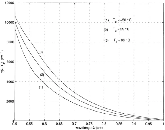
Fig. 3. as a function of and .
The quantum efficiency is then defined by the sum of the deple-tion region efficiency and back region efficiency
. With reference [10], and are given by
(9)
(10)
where , , and are respectively electron diffusion length in region (mm), substrate length (mm), and limit of deple-tion region (mm). represents the absorption photons coeffi-cient in silicon part (see formula in Appendix). Fig. 3 shows the evolution of this coefficient versus the wavelength at different temperatures. It decreases with an increasing wavelength and a decreasing temperature.
Therefore, the quantum efficiency of the detector is defined as a function of the wavelength and the temperature owing to absorption coefficient characteristics
(11)
where and are variable ( and ).
To model the quantum efficiency of the detector, we have to determine the internal parameters ( , , and ) of the de-tector. However, these parameters can generally not be accessed easily. One solution can be to measure the quantum efficiency and to fit the parameters of model (11). Another way to deal with this problem is to correct the constant value of the quantum efficiency known at a reference temperature with a law versus the wavelength and the temperature, as shown in (12)
(12) In NIR spectral band, the expression of is obtained from re-lation (11) and is defined by a macroscopic diffusion law, as follows:
(13) where is equal to 1 when and 1 on the contrary, while is given by
(14) where:
• , and
are respectively maximum and minimum wave-lengths of NIR spectral band ( ,
. is the energy gap (see formula in [11]).
Fig. 4. Noise transfer diagram.
• , is the
maximal detector temperature.
Finally, is a constant raised to power of normalized detector temperature . To obtain a ratio of 1 when
, we divide this term by 2. We get
(15) According to the first step of the determination of radiometric model, we compute the relation (12) at an effective wavelength
(16) From model (16), the temperature-signal relation (7) is modified as follows:
(17) where is a constant .
C. Coefficient D Model: Temporal Source Noise
We model coefficient by the sum of a constant and a variable scaling the temperature . is associated with an offset and with noise sources independent of temperature. We assume that noise is independent of signal level and spatial variations. Therefore, we get
(18) Many books and articles (i.e., [12]), describe noise sources depending on the detector temperature. We have represented the main ones on Fig. 4.
The main source noise comes from dark current generated by thermal generation in silicon. It has been shown that the mean background dark current level increases with the temperature
(Kelvin) and the integration time , as follows:
(19) where and are constant ( in silicon device).
Considering zero as the mean value of the reset noise, we add to the model (19) a linear dependence with temperature which comes from a drift of electronic components. Then, the mean
value of the digital output fluctuates with temperature, as follows:
(20) where and are constant .
D. Conclusion of Radiornetric Model Expression
Finally, (21) describes our complete radiometric model with nine parameters ( , , , , , , , , and ) which must be fitted during a calibration procedure
(21) where
constant
E. Radiometric Model Calibration
First, from the CCD camera model (21), we estimate the de-pendence of the output signal noise fl function of the detector temperature to fix the , , and parameters. Then, to fit missing parameters, the CCD camera has been calibrated using blackbody temperatures from 320 to 460 C intervals with de-tector temperature variation range 30 52 C.
On our experiments, we have tested several kinds of CCD cameras but we present only the results for the VHR 2000 CCD camera manufactured by Digital Vision. The CCD is a Sony
array of
pixels. This camera has a linear response with exposure time. We add Kodak Wratten 87C near infrared selected filter. All ex-perimental tests have taken place in a dark environment where the detector temperature was regulated with an air-condi-tioned enclosure.
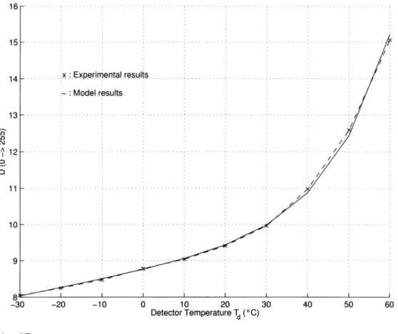
1) Observations of System Noise: In a dark environment and
when the detector temperature is adjusted between 30 and 60 C, we compute the mean value of the digital image. Considering an exposure time of 20 ms and a unitary gain , Fig. 5 shows a linear evolution for until temperature reaches 20 C. Above this temperature, increases exponen-tially mainly because of current noise. By fitting equation (18) to these values, we have deduced , , and parame-ters which are provided in Table I.
This model allows to estimate correctly the noise fluctuations for our uncooled CCD camera. Note that long exposure time re-quires a frame integration time concept. Charges are collected simultaneously but are read out alternately. Changing the gate voltage shifts the image centroid by half a pixel in vertical di-rection. This creates 50% overlap and therefore pixel sensitivity is doubled. This effect leads to an average of the noise.
Fig. 5. as a function of .
TABLE I
PARAMETERSVALUES OFMODEL(18)
Fig. 6. Experiment for radiometric calibration.
2) Temperature Calibration: In order to estimate the
missing parameters of model (21), we have directly illuminated the camera by a nearly spatially uniform blackbody (see Fig. 6). In order to cover a maximum of pixels, we have used a black-body with a large cavity (64-mm aperture). The temperature range is from 20 to 550 C. For a focal length of 8 mm, a F-number N of 1.4, an integration time of 360 ms, and an output amplifier gain of 1.41, we have computed the mean
Fig. 7. (1) Black-body uniform region.
value over a number of repeated image central regions (see Fig. 7). Within these experimental conditions, a value of over the range [0–255 Gray Levels] involves a black-body temperature range from 300 to 460 C. Of course, with a lower time exposure value, it is possible to increase the blackbody temperature without signal saturation.
Using these experimental points ( , ), the calibration pro-cedure to estimate the , , , , , and parameters of model (21) is as follows.
1) For the reference detector temperature : and determination.
Fig. 8. Calibration and verification curves for different .
Usually, the manufacturer gives data at a reference tem-perature of 20 C. In this case, the correction func-tion of the detector temperature is a unitary function in model (21). Curve 1 of Fig. 8 shows exper-imental points and model with and estimated pa-rameters.
2) For a different temperature : , , , and de-termination.
With a temperature different from , knowing and parameters, we can estimate the parameters of the function . The results of experiment and estima-tion procedure obtained with a detector temperature of 50 C.
3) Experimental verification of the model (21).
Considering the previous fitted parameters of model (21) and for a different value of 30 C, curve (3) of Fig. 8 represents experimental and computed results. The difference between experimental and calculated curve is lower than 1% of object temperature. Including all uncer-tainties, the model (21) with fitted parameters provided in Table II can be accepted.
F. Performances
Our experiments have taken into account detector tempera-ture variations in the radiometric model (21) over a range from 30 to 50 C. We model effects related to detector temperature in quantum efficiency due to variation in light absorption. In the reference of absorption coefficient formulas [13], the model can
TABLE II
PARAMETERSVALUES OFMODEL(21)
be extended to detector temperature lower than 30 C down to 50 C. At the other end, for temperatures higher than 50 C up to 80 C (CCD detector is still operating), no experiment shows the validity of the model. However, we can observe a high level of dark current (see Fig. 5). Knowing the detector temperature with an external sensor, the radiometric model (21) allows ob-ject temperature correction of 25 C for a gray level value of 100 (see Fig. 8).
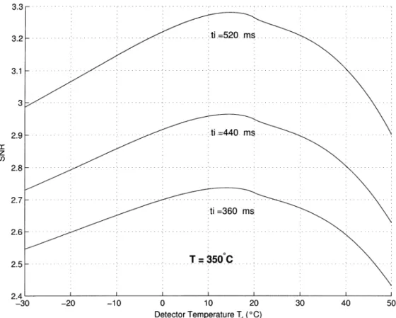
Particularly, in a measurement context, it is important to qualify the radiometric model performances in terms of signal-to-noise ratio (SNR) and noise equivalent temperature difference (NETD) as functions of detector temperature . Our goal described in the introduction, is to measure a low object temperature of 350 C with uncertainty value of 25 C. At this object temperature, Fig. 9 illustrates the SNR as a function of the temperature detector for different exposure time. The signal is provided by model (21) and the square root of the noise variance comes from the model (18). We observe a maximum SNR at a detector temperature of 18 C. Below this temperature value, the quantum efficiency limits the SNR value. At high detector temperature, dark current dominates and the SNR decreases. The NETD criterion is defined as the ratio of the standard deviation noise to the sensitivity that
Fig. 9. SNR as function of .
represents the derivative radiometric model (21) in function of object temperature . We compute it for an object temperature of 350 C. The result of NETD versus temperature and for different exposure time is plotted in Fig. 10. In the same way, NETD curves present also a minimum at detector temperature of 18 C. For a low detector temperature, sensitivity increases more than noise. On the contrary, for a high detector temper-ature, noise dominates.
As a conclusion, high detector temperatures degrade camera performances, but it is possible to adjust exposure time to respect values of SNR or NETD. For example, at reference detector temperature, to measure over the range from 350 to 1000 C with SNR higher than 2 and an NETD value always higher than 8 C, five exposure times are required over the range from 0.36 s to 1/10 000 s. The value of F-number and amplifier output gain are the same as those used in experiments.
III. GEOMETRICMODEL
This section describes the geometric model of the imaging system (optical lens, camera, and digital card). After an overview of the “pin-hole” model used in our applications, we define their extrinsic and intrinsic parameters to be calibrated. Extrinsic parameters describe the transformation of the object 3-D frame into the camera 3-D frame. The transformation of the latter frame into the image two-dimensional (2-D) frame is expressed by intrinsic parameters. They depend on optic perspective projection and detector CCD spatial resolution. By studying the MTF, we examine the influence of spectral
band and detector temperature on the spatial resolution. This analysis shows that intrinsic parameters depend on spectral band and detector temperature. In this section, we do not discuss the accuracy of intrinsic parameters in function of 3-D error models or 2-D errors introduced by the target detection in the camera image [14].
A. “Pin-Hole” Model
The basic assumption of the “pin-hole” model is that the lens center is the intersection of all optical beams. We as-sume that the image plane (or CCD detector plane) is perpen-dicular to optical axis . Fig. 11 illustrates the basic geometry of the pin-hole camera model.
represents the object 3-D frame, while de-notes the camera 3-D frame and is the image 2-D frame. Finally, is the principal point, or the optical center projection on the CCD detector plane.
Three steps are required to compute the transformation from a point ( , , ) in to a point in .
1) Rigid body transformation (rotation and translation ) of the object coordinates ( , , ) in to camera coordinates ( , , ) in .
2) Perspective projection with center , axis and ratio (distance between the CCD detector and the optical center), of the 3-D point ( , , ) into an image point ( ,
, ) expressed in the camera 3-D frame.
3) Transformation of camera coordinates ( , , ) into 2-D image frame coordinates ( , ) using an origin transfor-mation ( , ) in image plane and a space sampling
ac-Fig. 10. NETD as function of .
Fig. 11. Object and camera coordinate system.
cording to the pixel sizes and (considering pixels as adjacent in CCD array). The dependence of pixel sizes on wavelength and detector temperature will be discussed in paragraph III-B.
By combining these three steps, (22) relates the transforma-tion of the 3-D object into the 2-D image frame
(22) Model (22) involves 12 extrinsic parameters (nine for rotation and three for translation ) and four intrinsic parameters [ , , , )]. To simplify the presentation, we do not introduce in this paper the lens dis-tortion correction step described in [15]. We use this correction in our applications.
The model calibration described in [8] or [16] involves a com-putation of the camera extrinsic and intrinsic parameters based
Fig. 12. Diffusion influence.
on several points which object coordinates ( , , ) in the 3-D object frame are known and which image coordinates ( , ) are measured. These points are extracted from several im-ages of a specific object (planar calibration pattern), moved in front of the camera.
For robotic applications, self-calibration methods [17] have been proposed to recover these parameters on line, using a weak camera model. For our measurement applications, we apply a strong calibration method, which requires two steps: a) using
Fig. 13. MTF as a function of .
initial estimates of the intrinsic parameters computed from the camera characteristics, the object pose computation [18] gives estimates for the extrinsic parameters for each image acquired on the calibration object. b) Then, from the initial guesses, a non linear minimization method (including the estimation of the distortion coefficients) allows to improve the estimation of these parameters. A basic hypothesis for this procedure is that focal length and pixel sizes et remain constant. If it is not the case (active camera or fluctuations according to the wavelength and to the detector temperature), they must be estimated again. The metrology applications require very accurate estimates of the camera parameters: therefore we have to verify if in-trinsic parameters, especially and , are changing with spectral band and detector temperature fluc-tuations. The MTF of the camera characterizes the optic effects and how the discrete locations of detector elements ( , ) sample spatially the scene in function of wavelength and de-tector temperature.
B. Camera MTF
The complete MTF of the camera is the product of the optic MTF (MTF ) and the detector MTF (MTF ), that is
MTF MTF MTF (23)
1) Optic MTF : With reference to [19], MTF in the
hori-zontal or vertical direction of a radial symmetric optical system
with a clear circular diffraction-limited aperture illuminated monochromatically is given by
MTF
(24)
where is the cutoff frequency of the optical system . In NIR spectral band, with an F-number equal to 1.4, MTF is close to 1 (0.998–0.978). The camera MTF can then be approximated by MTF
MTF MTF (25) The camera cutoff frequency is equal to the detector cutoff frequency .
2) Detector MTF : CCD detector is a spatial sampler of a
horizontal frequency (respectively vertical ) of the input signal. The highest CCD horizontal frequency reproduced is the Nyquist horizontal frequency (respectively vertical ). It is mandatory that the input signal frequency are inferior to Nyquist frequency to respect Shannon theorem and to avoid spa-tial aliasing. In metrology applications, the Nyquist frequency is the band-limit or the system cutoff frequencies which is defined as half an inverse pixel dimension:
Fig. 14. MTF as a function of .
adjacent. We note that the detector cutoff frequency decreases when the cell area increases.
Moreover of the influence of the detector geometry, in NIR spectral band, the photons absorption occurs at increasing depths along substrate detector depth . The absorption law approaches an exponential law [ ] where the coefficient absorption in the silicon decreases with an increasing wavelength (see Fig. 3). However, the depletion region size is finite (see Fig. 2) and the majority of long wavelength photons will be absorbed outside of the depletion region. An electron generated in substrate will experience a 3-D random walk until it recombines or reaches the edge of neighbor depletion region. In the last case, this phenomenon, called diffusion, creates a response that overlaps other pixels (see Fig. 12 in reference of [13]).
Finally, in NIR spectral band, the detector MTF (MTF ) re-sults of the product of the geometric MTF (MTF ) by the dif-fusion MTF (MTF ), and it is expressed by
MTF MTF MTF (26) According to [20], the geometric MTF of a single CCD cell is given by
MTF
(27)
In order to simplify the expression, we compute the MTF only in one dimension for the horizontal direction . Therefore, we denote the horizontal input frequency as and hori-zontal Nyquist frequency as . For , the MTF value is 0.637.
For a front illuminated CCD, the diffusion term MTF in reference of [21] can be written as
MTF (28)
where the factor is the spatial frequency-dependent compo-nent of diffusion length and
is the depletion width (see Fig. 2).
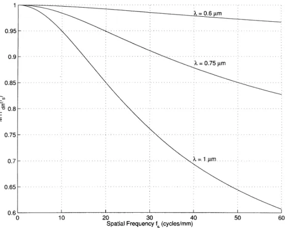
Let us remark that the diffusion term MTF depends on the absorption coefficient as a function of wavelength and tem-perature as shown in Fig. 3.
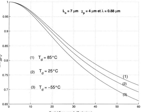
Fig. 13 shows MTF versus wavelength ( m, m). For short wavelengths m , MTF can be neglected and it approaches 1 (MTF MTF ). For the NIR spectral band m, the diffusion term MTF dominates in the MTF relation. As illustrated by Fig. 14, the diffusion term MTF decreases with the detector temperature.
As a conclusion, in visible spectral band, we can approximate the camera MTF with only the geometric MTF (MTF ) of the detector
Fig. 15. Bar test target.
Fig. 16. Definition of and .
But, in NIR spectral band, the cameraMTF must be expressed as the product of the geometric MTF (MTF ) by the diffusion MTF (MTF )
MTF MTF MTF MTF (30) With the same value of MTF (MTF ), the camera cutoff frequency is lower in NIR than in visible spectral band. In addition, its value decreases with the detector temperature. Finally, the pixel effective sizes are higher in NIR than in visible spectral band.
C. Experimental Results
Although the camera MTF is defined for sinusoidal signals, the square wave (see Fig. 15) is the most popular test target. The system response to a square-wave target is the contrast transfer function (CTF)
CTF (31)
where and are respectively maximum and min-imum signal levels of white and black bar test (see Fig. 16). To obtain the relationship between square wave and sinusoidal am-plitude, we have to express the square wave as cosine series. The
output amplitude is an infinite sum of input cosine amplitudes modified by MTF
CTF MTF MTF (32) where represents the fundamental frequency of the square wave.
For bar target with spatial frequency above of fre-quency computed to MTF , we can write the camera MTF from the measured CTF, as follows:
MTF CTF (33) After measuring the CTF of the VHR 2000 CCD camera tested in paragraph II-E, from (33) we compute the MTF and we com-pare the cutoff frequency (for a value of 0.637 of the MTF) in visible and in NIR spectral band. We also examine the influence of the detector temperature on the MTF.
1) MTF as a Function of Wavelength: Using experimental
and model results (MTF, ) plotted in Fig. 17, we can compute the cutoff frequency , as follows.
• In visible spectral band (MTF ):
For a value of 0.637 of the MTF, the value of the cutoff frequency is 45.3 mm . From relation , it easily follows that the value of the detector width is 11 m. The value is different from the manufacturer’s
8.6 m due to a low pass filter with a cutoff frequency lower than Nyquist frequency to satisfy the Shannon sampling theorem.
• In NIR spectral band:
Considering experimental results plotted in Fig. 17, MTF produced in NIR is lower than MTF produced in visible spectral band. We can estimate and parameters of the diffusion term MTF (28) in the model (30). The values are provided in Table III. As a result, the value of the cutoff frequency is 30.50 mm leads to a detector width value of 16.39 m.
We note that the diffusion length value is small. The lim-ited diffusion in substrate can be explained at least in part by a likely epitaxial layer. This fact can be also ascribed to an inade-quate 2-D diffusion model to explain 3-D diffusion mechanisms. As a conclusion, in NIR spectral, MTF decreases and it is equivalent to work with detector sizes 1.34 times higher.
2) MTF as a function of the detector temperature: To take
into account the effects of the detector temperature, consid-ering previous values of and parameters (see Table III), we compute the absorption coefficient (see formulae in Ap-pendix) as a function of detector temperature ranging from 50 to 80 C. From these computations and the model (30) in NIR spectral band, we obtain the MTF values versus temper-ature . For MTF value of 0.637, we can deduce the cutoff frequency and compute the detector width as a function of . The Fig. 18 shows a linear decreasing of the detector width with a detector temperature increasing . We can infer the following linear model:
Fig. 17. Experimental verification of MTF. TABLE III
PARAMETERVALUES OFMODEL(28)
where is a parameter which value has been obtained from the experimental points plotted in Fig. 18.
D. Performances
By studying the MTF as a function of wavelength, we notice that the spatial resolution of the CCD detector decreases with an increasing of wavelength to account for diffusion phenomenon. To fit the intrinsic parameters of the “pin-hole” camera model, the system has been calibrated in NIR spectral band.
The same studies show an increasing of spatial resolution with detector temperature. We propose a correction law (34) of intrinsic parameters , and as a function of detector temper-ature . With a limited substrate detector by an epitaxial layer, the correction is less necessary than with a thick substrate de-tector (for example with the dede-tector Hamamatsu 5466). The model calibration has been tested in visible and in NIR spectral band with test points extracted from lozenge center. We esti-mate intrinsic parameters with method [16] and we obtain and , 1131.17, 1037.34 in visible and, respectively, 1139.53 and 1045.09 in NIR spectral band. The localization error given by method described in is 0.1 mm at an observation distance of 1 m. This experiment should be conducted many times to verify parameters dispersion.
IV. TWOMODELSINTERESTS
In the two previous sections, we have presented radiometric and geometric calibration procedures for an uncooled CCD camera. We emphasize on the fluctuations of the camera parameters with respect to the detector temperature and to the wavelength.
In this section, we show the interest of these two models in order to improve some measurements on a hot object, which can be in any situation in the view field of the camera. In fact, variable orientation and distance of a hot object could be estimated by a 3-D localization. For monocular vision (only one camera), it could be impossible to locate a single hot point. This point must be associated to a surface belonging to an object. The object position with respect to the camera, can be computed only if the 3-D geometric model of the object has been previ-ously learnt. For an application concerning the monitoring of free-form objects, a rigid visual pattern can be fixed on the ob-ject to make this localization easier by using a classical method [8]. For multiocular vision (passive stereo vision), a hot point could be detected and localized using triangulation methods. But, it is required that this point is in the view field of the two cameras. A first estimate on the radiometric attributes, com-puted without any knowledge on the orientation and the dis-tance, could be used as a stereo-matching criterion. Then, once the point distance is known, the orientation could be computed from local planar approximations, and the radiometric attributes could be refined using the equation (36).
Fig. 18. as a function of .
Fig. 19. Description of geometric situation.
In fact, the Fig. 19 shows the geometric situation between a hot source (black body) of area and sensor of area through the optical system of focal length and area . The hot source sees optical area under the solid angle
(in the same way detector sees optical area under the solid angle ). is the angle between the axis
and the source normal (respectively, with detector normal ). In measurement situation, angles ( , ) are different from zero, the optical system is not focused and we have to correct the digital output signal measurement by the geometric situation, as follows:
(35)
where , , and are provided by localization methods. After correction of in relation (35), the radiometric model is inverted to measure the object temperature with respect to the corrected intensity . Relation (36) provides real object temperature
(36)
With any hot source, we must also modify by emissivity value at effective wavelength . It is better to work with short wavelength to decrease uncertainty on this emissivity. For ex-ample, in [22], a relative emissivity uncertainty of 20% leads to a relative temperature uncertainty of 1.2% at wavelength m and of 12% at m, respec-tively.
V. CONCLUSION
In this paper, we have described radiometric and geometric models taking into account detector temperature variations based on an uncooled low cost CCD camera operating in the NIR.
Using physical COD properties, we have analyzed the influence of wavelength and detector temperature fluctuations on the radiometric model [see (21)] usually used in cooled in-frared thermographic systems. The temperature fluctuations (a) involve quantum efficiency variations due to light absorption and modifications of diffusion mechanisms [see (13)] and (b)
affect sensor noise levels [see (18)] (especially dark current). Experimental calibration results confirm the radiometric model (21) with a COD camera based on a Sony detector over a detector temperature range of 30 to 50 C. Knowing the detector temperature with an external sensor, this model allows us to correct the object temperature by 10% (see Fig. 8) to compensate detector temperature fluctuations of 80 C. To ob-tain the same performances in function of detector temperature variation in terms of SNR or NETD, we propose to adjust the exposure time of the CCD detector. Figs. 9 and 10 show SNR and NETD, respectively, as a function of detector temperature . An optimal point of both criteria at a detector temperature of 18 C can be exhibited. Moreover, we can measure a hot object over the temperature range of 350 to 1000 C with a precision lower than 25 C at 350 C.
On the other hand, by studying the MTF, we have analyzed the detector CCD spatial resolution properties in function of spectral band and detector temperature fluctuations. This anal-ysis establishes that the spatial resolution decreases in NIR spec-tral band due to a diffusion term MTF [see (28)]. This term (MTF ) depends on the absorption coefficient that is itself wavelength and detector temperature dependent. Therefore, we prove that the spatial cutoff frequency of a CCD detector de-creases when the wavelength inde-creases and the detector tem-perature decreases. As the cutoff frequency is inversely pro-portional to pixel size , it is equivalent to work with an effective pixel size which is wavelength- and de-tector-temperature dependent. The properties are explained in geometric model (22). First, to consider wavelength effects, we have to calibrate the model in NIR spectral band to fit intrinsic parameters with effective pixel sizes. Then, using model (34), the detector temperature correction can be applied in geometric model (22) to compensate a relative error of 0.01% in a dis-placement of 100 mm. This error could be higher with a thick substrate detector with greater diffusion effects.
We have characterized a low cost sensor to measure surface temperature field and dimensional characteristics. It could also be used in thermal treatment process of tools [23] or super plastic forming (SPF) of Titanium alloy sheets [24].
APPENDIX
According to [13], absorption photons coefficient is given as follows.
(a) For a photon energy between 1.2 and 2.2
(37) (b) For a photon energy between 2.2 and 2.5
(38)
ACKNOWLEDGMENT
The authors would like to thank J. J. Orteu for his helpful comments, as well as Referee.
REFERENCES
[1] Y. Le Maoult, S. Baleix, P. Lours, and G. Bernhart, “Application indus-trielle de la thermographie infrarouge au comportement des outillages de formage superplastique,” in Congrès National sur les applications de la
thermographie dans les industries mécaniques. Senlis, France, 1999.
[2] D. Garcia and J. J. Orteu, “3D deformation measurement using stereo-correlation applied to the forming of metal or elastomer sheets,” in Int. Workshop Video-Controlled Mater. Testing In-Situ
Microstruc-tural Characterization. Nancy, France, Nov. 1999.
[3] S. Claudinon, P. Lamesle, J. J. Orteu, and R. Fortunier, “Continuous in-situ measurement of quenching distortions using computer vision,”
J. Mater. Processing Technol., vol. 122, pp. 69–81, Mar., 2002.
[4] G. J. Zissis, Ed., The Infrared & Electro-Optical Systems
Hand-book. Bellingham, WA: SPIE, 1992, vol. 1.
[5] F. Moreau, “Thermographie Proche Infrarouge par Caméras CCD et Application aux Composants de Premiére Paroi du Tokamak TORE SUPRA,” Ph.D. dissertation, Univ. Saint Jérôme, Marseille, France, June 1996.
[6] F. Mériaudeau, E. Renier, and F. Truchetet, “Uncertainty committed on temperature measurement,” in Congr. Int. Métrologie, vol. 1, Nimes, France, Oct. 1995, pp. 189–194.
[7] E. Healey and K. Ragava, “Radiometric CCD camera calibration and noise estimation,” IEEE Trans. Pattern Anal. Machine Intell., vol. 16, p. 267, Mar. 1994.
[8] R. Y. Tsai, “A versatile camera calibration technique for hight-accuracy 3D machine vision metrology using off-the-shelf tv cameras and lenses,”
IEEE J. Robot. Automat., vol. RA-3, Aug. 1987.
[9] P. Saunders and T. Ricolfi, “The characterization of a CCD camera for the purpose of temperature measurement,” in Int. Symp. Temperature
Thermal Meas. Ind. Sci. (TEMPMEKO), Torino, Italy, Sept. 1996, pp.
329–334.
[10] M. Orgeret, Les Piles Solaires, le Composant et ses
Applica-tions. Paris, France: Editions Masson, 1985.
[11] F. H. Gaensslen, V. L. Rideout, E. J. Walker, and J. J. Walker, “Very small MOSFET’s for low temperature operation,” IEEE Trans. Electron
Devices, vol. ED-24, pp. 218–229, Mar. 1977.
[12] 75 222“Tech. Rep.,” Texas Instruments Incorpored, Central Research Laboratories, Dallas, TX, May 1975.
[13] G. Roiland, “Etude des variations de rendement quantique interne d’un détecteur CCD en fonction de la température,” Rev. Phys. Appliquée, no. 20, pp. 651–659, Sept. 1985.
[14] J. M. Lavest, M. Viala, and M. Dhome, “Do you really need an accu-rate calibration pattern to achieve a reliable camera calibration,” in Eur.
Conf. Comput. Vision (ECCV), vol. 1, Freiburg, Germany, June 1998,
pp. 158–174.
[15] G. Weng, S. Ma, and M. Herniou, “Camera calibration with distorsion models and accuracy evaluation,” IEEE Trans. Pattern Anal. Machine
Intell., vol. 14, no. 10, pp. 965–980, Oct. 1992.
[16] M. Devy, V. Garric, and J. J. Orteu, “Camera calibration from multiple views of a 2D object, using a global non linear minimization method,” in
IEEE/RSJ Int. Conf. Intell. Robots Syst. (IROS), Grenoble, France, Sept.
8–12, 1997.
[17] A. Fusiello, “Uncalibrated euclidean reconstruction a review,” Image
Vision Comput., vol. 18, no. 6–7, pp. 555–563, May 2000.
[18] M. A. Abidi and T. Chandra, “A new efficient and direct solution for pose estimation using quadrangular targets algorithm and evaluation,”
IEEE Trans. Pattern Anal. Machine Intell., vol. 17, p. 534, May 1995.
[19] M. C. Dudzik, Ed., The Infrared 81 Electro-Optical Systems
Hand-book. Bellingham, WA: SPIE, 1992, vol. 4.
[20] G. C.Gerald C. Hoist, Ed., CCD Arrays Cameras and
Dis-plays. Bellingham, WA: SPIE, 1998.
[21] D. H. Sieb, “Carrier diffusion degradation of modulation transfer func-tion in charge coupled imagers,” IEEE Trans. Electron Devices, vol. ED-21, pp. 210–217, may 1974.
[22] J. Martinet, La Mesure des Températures par Rayonnement
Ther-mique. Paris, France: Bureau National de Métrologie, 1981. [23] S. Claudinon, “Contribution à L’étude de la Distorsion des Aciers au
Traitement Thermique : Suivi en Continu par Vision Artificielle et Sim-ulation Numérique,” Ph.D. dissertation, Ecole des Mines Paris, Février, France, 1999.
[24] S. Baleix, “Oxydation et Écaillage D’alliages Réfractaires Moules Pour Outils de Formage Superplastiqne,” Ph.D. dissertation, Université Paul Sabatier, Toulouse, France, Dec. 1999.
Thierry Sentenac received the M.S. degree in computer science from INP,
Toulouse, France, in 1992. He is currently pursuing the Ph.D. degree at the Lab-oratoire d’Analyze et d’Architecture des Systèmes (LAAS)-CNRS, Toulouse.
From 1992 to 1995, he was a Research Engineer at LAAS-CNRS. Since 1995, he has been an Associate Professor and he is Head of the Electrical Engineering Department, Ecole des Mines d’AIbi, Albi, France, specializing in process engi-neering. His current research interests cover CCD image processing, computer vision, and optoelectronics.
Yannick Le Maoult received the M.S. degree in physical measurements from
INP, Grenoble, France, in 1987, and the Ph.D. degree from the University de Provence, Marseille, France, in 1992.
Since 1992, he has been an Associate Professor at the Ecole des Mines d’Albi, Albi, France, and a French Grande Ecole specializing in process engineering. He is a member of the Computer Vision and IR Thermography Group (Mate-rial Research Center) and his fields of interest include radiative transfer, optical measurements, metrology, and inverse methods. Particularly, he is involved in infrared measurements, such as thermography or pyrometry, applied to material processing or reactive flows.
Guy Rolland has been an Engineer with the French National Center for Space
Research (CNES), France, since 1978. From 1978 to 1987, he worked in the field of characterization and physical modeling of CCDs and other detectors for earth observation and scientific satellites. From 1987 to 1999, he concentrated on the field of modeling CCD and active electronics components by means of finite elements methods (process and devices simulations). Since 1999, he has been working in the field of radiation effects on components and systems. One of his research themes today is the effect of space radiation on CCDs. He also teaches physics of semiconductors imaging and components in Toulouse, France, university and engineer schools.
Michel Devy received the M.S. degree in computer science engineering from
IMAG, Grenoble, France, in 1976, and the Ph.D. degree from the Laboratoire d’Analyze et d’Architecture des Systèmes (LAAS)-CNRS, Toulouse, France, in 1980.
Since 1980, he has participated in the Robotics and Artificial Intelligence Group of LAAS-CNRS. His research is devoted to the application of computer vision in automation and robotics. He has been involved in numerous national and international projects regarding manufacturing applications, mobile robots for space exploration or for civil safety, and 3-D vision for intelligent vehicles or medical applications. He is now Research Director at CNRS, Head of the Perception Area in the Robotics Group, and his main scientific topics concern perception for mobile robots in natural or indoor environments.