HAL Id: inria-00432129
https://hal.inria.fr/inria-00432129
Submitted on 13 Nov 2009
HAL is a multi-disciplinary open access
archive for the deposit and dissemination of
sci-entific research documents, whether they are
pub-lished or not. The documents may come from
teaching and research institutions in France or
abroad, or from public or private research centers.
L’archive ouverte pluridisciplinaire HAL, est
destinée au dépôt et à la diffusion de documents
scientifiques de niveau recherche, publiés ou non,
émanant des établissements d’enseignement et de
recherche français ou étrangers, des laboratoires
publics ou privés.
Deployment Schemes for Mobile Sensor Networks
Guang Tan, Stephen Jarvis, Anne-Marie Kermarrec
To cite this version:
Guang Tan, Stephen Jarvis, Anne-Marie Kermarrec. Connectivity-Guaranteed and Obstacle-Adaptive
Deployment Schemes for Mobile Sensor Networks. IEEE Transactions on Mobile Computing, Institute
of Electrical and Electronics Engineers, 2009. �inria-00432129�
Connectivity-Guaranteed and Obstacle-Adaptive
Deployment Schemes for Mobile Sensor
Networks
Guang Tan, Stephen A. Jarvis, and Anne-Marie Kermarrec
Abstract—Mobile sensors can relocate and self-deploy into a network. While focusing on the problems of coverage, existing
deployment schemes largely over-simplify the conditions for network connectivity: they either assume that the communication range is large enough for sensors in geometric neighborhoods to obtain location information through local communication, or they assume a dense network that remains connected. In addition, an obstacle-free field or full knowledge of the field layout is often assumed. We present new schemes that are not governed by these assumptions, and thus adapt to a wider range of application scenarios. The schemes are designed to maximize sensing coverage and also guarantee connectivity for a network with arbitrary sensor communication/sensing ranges or node densities, at the cost of a small moving distance. The schemes do not need any knowledge of the field layout, which can be irregular and have obstacles/holes of arbitrary shape. Our first scheme is an enhanced form of the traditional virtual-force-based method, which we term the Connectivity-Preserved Virtual Force (CPVF) scheme. We show that the localized communication, which is the very reason for its simplicity, results in poor coverage in certain cases. We then describe a Floor-based scheme which overcomes the difficulties of CPVF and, as a result, significantly outperforms it and other state-of-the-art approaches. Throughout the paper our conclusions are corroborated by the results from extensive simulations.
Index Terms—Sensor Networks, Mobile, Deployment, Connectivity.
✦
1
INTRODUCTION
In a mobile sensor network the sensors are able to relo-cate and self-organize into a network. The mobility and self-management of sensors are desirable for many appli-cation scenarios, including remote harsh fields, disaster areas, or toxic urban regions, where manual operations are unsafe or burdensome. In this paper we consider the following self-deployment problem: Given a target sensing field with an arbitrary initial sensor distribution, how should these sensors self-organize into a connected ad hoc network that has the maximum coverage, at the cost of a minimum moving distance?
There have been a number of proposed solutions to this problem, including that based on the concept of potential fields [6] or virtual forces [21]. This approach imitates the behavior of electro-magnetic particles: when two electro-magnetic particles are too close in proximity, a repulsive force pushes them apart. Applied to a sensor network, this method helps move sensors from high density to low density areas, thereby minimizing sensing overlap and improving the overall network coverage. Another commonly used approach relies on the use of Voronoi Diagrams (VDs) [4] [5] to partition the field into many sub-areas, one for each sensor, allowing sensors • Guang Tan and Anne-Marie Kermarrec are based at INRIA-Rennes,
Rennes, France. E-mail: {gtan, anne-marie.kermarrec}@irisa.fr
• Stephen A. Jarvis is with the Department of Computer Science at the University of Warwick. Coventry, CV4 7AL, UK. E-mail: [email protected]
Manuscript received 2008.
to move to maximize coverage in its own sub-area. A combination of these two approaches is also possible; see [14].
While existing methods prove to be effective under certain models, they have several problems in prac-tice. First, they assume that a sensor can easily detect all (or most) of its Voronoi neighbors through local communication. This assumption may not however be satisfied in a real network, because the communication range of a sensor may not be large enough to cover all Voronoi neighbors. An incomplete view of the Voronoi neighbors may result in very inaccurate VDs being con-structed. Consequently, significant sensing overlaps or voids among sensors may be ignored, leading to poor network coverage. Figure 1 illustrates the impact of com-munication range on the construction of Voronoi cells. In Figure 1(a), O’s communication range is such that it will detect all of its Voronoi neighbors, enabling it to construct a correct Voronoi cell; in Figure 1(b) however, the shorter communication range only covers four of the Voronoi neighbors, yielding an incorrect Voronoi cell.
A second problem with existing studies is that when concentrating on the motion planning of sensors, they tend to assume that the network remains connected throughout the process of sensor relocation. However, the implicit assumption that the network connectivity can be guaranteed by a high node density, or a large communication range, does not hold in general; network partitions can still occur in a dense network. As a critical requirement for a network to function normally, connec-tivity must be considered in protocol design. A third
problem that we observe with existing schemes is that when planning sensor relocation to increase coverage, most existing studies assume that the sensing field is obstacle-free (e.g., [13] [18]). This greatly simplifies the motion planning and optimization problem, but in so doing it is clear that many real-world environments (a metropolitan area with buildings, or a rural environ-ment with plants and water etc.) that naturally have obstacles or holes, render such schemes ineffectual. This significantly weakens the potential applicability of such approaches.
In this paper, we present new schemes that are not governed by the above simplifying assumptions, and thus adapt to a much wider range of application scenar-ios. While maximizing sensing coverage, our distributed schemes also aim to achieve three additional goals: (1) to achieve connectivity for a network with an arbitrary ini-tial distribution, communication/sensing range, or node density; (2) to minimize moving distance, which dom-inates energy consumption in the deployment process; (3) to be able to work without any knowledge of the field layout, which can be irregular and have obstacles of arbitrary shape. This is important for deployment in an environment whose layout is not fully known in advance. The lack of topological knowledge also makes a central server-based deployment solution infeasible.
To the best of our knowledge, no published work ad-dresses all these issues simultaneously. Optimization of the multiple objectives (coverage and moving distance) under the constraint of global network connectivity for general network topologies is known to be a challenging task; even sub-problems of this have been shown to be difficult. For instance, Wang et al. show that introducing a minimum number of sensors to completely cover a target area is strongly NP-hard [15]. In view of the com-plexity of the problem, our design is heuristic-based and supported by comprehensive experimental evaluation.
Our first solution is called the Connectivity-Preserved Virtual Force (CPVF) scheme, which is an enhanced form of the virtual-force-based method with the additional consideration of the connectivity requirements. We show that the localized communication, which is the very reason for its simplicity, results in poor coverage in cases of small communication ranges and obstacles. We then consider a Floor-based scheme (or FLOOR for short) which divides the field into fixed-height floors and en-courages sensors to maintain a particular floor-height level. The coverage expansion process of FLOOR can be regarded as being similar to the growth of a plant from the Vitis genus (e.g. a common vine). Simulations show that FLOOR overcomes all the difficulties of CPVF and several previous algorithms, and significantly out-performs them in terms of coverage, moving distance, and convergence time.
The remainder of this paper is organized as follows. Section 2 documents related work and Section 3 intro-duces preliminaries of the proposed schemes. Section 4 presents the CPVF scheme in detail; Section 5 describes
O
P P O
(a) (b)
Fig. 1. Impact of communication range on the construc-tion of Voronoi diagrams.
the FLOOR scheme.In Section 6 we evaluate the per-formance of a number of different schemes through extensive simulations. Finally, Section 7 concludes the paper.
2
RELATED
WORK
Sensor deployment problems have been studied in a variety of contexts. It is widely recognized that when deploying sensor networks, coverage and connectivity must be considered together. The authors in [17] provide a geometric analysis of the fundamental relationship between coverage and connectivity, and present pro-tocols to achieve a desired degree of coverage while maintaining network connectivity. They prove that when the communication range rcis at least twice the sensing
range rs, then coverage implies network connectivity.
The assumption rc ≥ 2rsgreatly simplifies the design of
coverage-oriented protocols (for instance, the location-free coverage protocol [19] and obtaining tradeoffs be-tween mobility and coverage [16]); at the same time this assumption also limits the protocol’s applicability. Bai et al. [1] first present a full picture of optimal deployment patterns that achieve both coverage and connectivity for general values of rc/rs. In particular, they show a
strip-based pattern that achieves asymptotically optimal cov-erage with one-connectivity, and for two-connectivity, some variants of the strip pattern are also proposed. In [2], the authors consider the same problem with a higher degree of connectivity. While these work provides useful guidelines for real network deployment, their analysis only considers an obstacle-free plane, therefore the results do not apply to a field with holes of general shape.
In a mobile sensor network, the mobility of sensor nodes provides the possibility for the nodes to self-organize to a network with desired properties from an arbitrary initial distribution. Howard et al. [6] employ the potential field method in sensor deployment, assum-ing a line-of-sight connectivity; that is, a sensor is always able to determine the location of nearby nodes. This actually requires special sensing ability or alternatively, a large communication range, in a non-dense network. Zou. et al. [21] propose a VF-based deployment scheme, which is centralized and only works for a small cluster of sensors.
In [14], Wang et al. present a set of VD-based schemes to maximize coverage. The VDs are used by sensors to detect coverage holes in their vicinities, and sensor locations are adjusted round by round so that the cov-erage is gradually improved. Other schemes that have employed VDs include [15] [14] [4] [5]. As previously described, this approach implicitly relies on a relatively large rc/rsto guarantee the construction of a correct VD.
This condition concerning rc/rs is not always satisfied
in practical scenarios, where rc/rs could be any value.
Furthermore, their studies do not consider the problems of connectivity and obstacles.
Yang et al. [18] use a grid-based network structure to detect low density areas, and then maximize sensing coverage through balancing the sensor distribution. The same structure is also used in [13] to identify redundant sensors. Unfortunately, a grid structure is feasible only for networks with relatively high densities, which, again, translate to a relatively large rc. In addition, both sets of
research require an obstacle-free field.
Liu et al. [10] study the dynamic coverage of a sensor network. They show that while the mean coverage at any given time instance remains unchanged, a larger area will be covered during a time interval because of sensor movement. A similar concept called sweep coverage is studied in [3]. Our work differs from theirs in that we consider only static coverage.
3
PRELIMINARIES
3.1 System assumptions
We assume that all sensors have the same communi-cation range rc and sensing range rs. Both ranges are
modeled as an isotropic unit disk, and sensors within rc of a sensor are called that sensor’s neighbors. As
is the case for many applications, a sensor can deter-mine another sensor’s location only by communication. (Relaxing this requirement only simplifies the design.) At any given time, a sensor knows its own position and can recognize the boundary of the obstacles within its sensing range. All sensors are also aware of the boundary of the sensing field. Sensors move in steps of variable size (or distance). In each step, a sensor moves in a straight line at a uniform speed for a fixed amount of time (e.g., 2 seconds), which we term a period and denote by T ; and at the end of that step, it decides the direction and size of the next step, and so on. The maximum moving speed is denoted by V .
We assume that the field is on a 2-D plane, which can contain any number of obstacles of arbitrary shape, as long as the field is connected; that is, any two points in the non-obstacle areas of the field can be connected by a continuous path. There is a reference point O known to all sensors, where O could be the location of the base station or some head sensor; all the sensors will try to connect to O either directly or via multi-hop links. Without loss of generality, we assume O is at (0, 0). The base station knows the total number of sensors in the
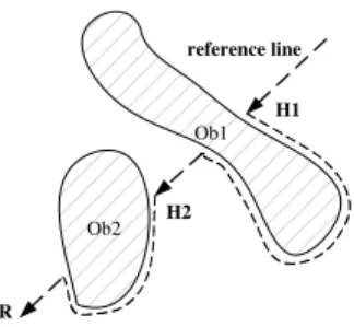
Ob2 Ob1 R reference line H1 H2
Fig. 2. An example of the BUG2 algorithm. The dashed line shows the path of a sensor moving to the point R. On its way toR, the sensor encounters two obstacles and moves around them using the right-hand rule.
network while other sensors do not. Sensors do not have a map of the sensor field.
3.2 Obstacle avoidance
We use Lumelsky and Stepanov’s path planning algo-rithm [11] called BUG2 to help a sensor move from a starting point Start to a destination point T arget in an environment with obstacles. Roughly speaking, this algorithm works as follows. The sensor initially moves along the straight line (Start, T arget), which we call the reference line, until it encounters an obstacle at some hitting point H; then, the sensor follows the boundary of the obstacle using the right-hand rule (i.e., the right hand maintains contact with the obstacle), until it gets back to the reference line at some point. Now, if the sensor finds that it is closer to the T arget than from H, and that it can make progress on the reference line, then it resumes its straight line walk toward the T arget; otherwise it continues to navigate around the obstacle. The above procedure repeats until the sensor reaches the T arget. BUG2 is shown to produce a path of length at most D +Pinili
2 , where D is the distance between Start and T arget, ni is the number of times the reference line
crosses the ith obstacle, and li is the perimeter of the
ith obstacle. For convex obstacles, BUG2 is essentially optimal. Figure 2 provides an example of this algorithm.
3.3 Lazy movement
With multiple hop communication, not all disconnected sensors need to move to get connected. We use a lazy movement strategy to reduce the unnecessary movement as follows. At the end of each step, a sensor checks its neighbors to see if there are any ahead of it (i.e., closer to its current destination); if so, then it chooses the nearest neighbor as its candidate path parent. A sensor with a path parent can stop moving for a period, in the hope that the path parent can become connected, thereby saving its own movement. A sensor can take a neighbor as a real path parent, only when that neighbor is not adopting the sensor itself as a path parent. When the field is irregular or has obstacles, it may be the case that two sensors are waiting for each other’s move indirectly.
In our scheme, if a sensor has not moved for a certain number of periods, it will check whether a loop exists. To do this it sends aPathParentInquirymessage once a
period to the parent path, which forwards the message to its own path parent if available, and so on. If the sensor finally receives such a message sent by itself, then it knows that a loop has been formed, and it simply resumes its suspended walk at the beginning of the next step; the disregarded path parent will not be taken as its path parent again. A sensor stops moving only when it enters the communication range of a connected sensor, at which time it takes the connected sensor as its parent and changes its own state to connected.
4
T
HE CONNECTIVITY-
PRESERVED VIRTUALFORCE
(CPVF)
SCHEMEThe traditional virtual force method has the advantage of local communication, coverage maximization capability, and adaptability to obstacles. Therefore our first design is based on this method. Our approach to achieving these three goals is to first guarantee network connectivity by having disconnected sensors move toward the base station to establish connectivity, during which time we try to minimize the moving distance; the virtual forces method is then applied to maximize coverage.
4.1 Achieving connectivity
Initially, all sensors are required to decide their states regarding connectivity. The sensors in the immediate vicinity of the base station know that they are connected. Those sensors then flood a message to the network, and sensors receiving such a message, becoming aware that they are also connected, further flood the message into the network (each sensor sends the message only once). After a certain period of time (for example, an estimate of the maximum possible multi-hop transmission delay between two sensors), if a sensor still has not received such a message, it can decide that it is disconnected. In this case, it will allow a small random time period to elapse after which it starts to move using the BUG2 algorithm (with the lazy movement strategy) toward the base station.
4.2 Maximizing sensing coverage
All sensors, upon becoming connected, start to move under the influence of virtual forces (VF) in order to maximize sensing coverage. Our goal is to preserve the network connectivity throughout this stage.
The use of virtual forces in our protocol is essentially the same as in previous work (e.g., [21]): the obstacles and neighboring sensors exert repulsive forces onto a sensor, and the sum of all forces determines the subse-quent direction of that sensor. In fact, the VF method is used in our scheme only for determining the direction to move in; the selection of step size needs special care in the interest of network connectivity and maximum
coverage: on the one hand, aggressive step sizes may push sensors beyond the communication range and thus cause network partitions; on the other hand, moving too conservatively may result in sensors being distributed far from evenly, which usually means poor coverage. Considering this, we need a sensor to be able to de-termine the maximum step size it can make without disconnecting the network, or the maximum valid step size, at the end of each step.
Suppose at time t, the beginning of some period, a sensor s needs to check whether a planned move will disconnect itself from a current neighbor s0, or
whether that move for s0 is valid. Since the network
is an asynchronous system, sensor s0 may be in the
middle of its own period, which we assume ends at time t0 ≤ t + T . Sensor s first obtains the information of s0’s
current moving direction, moving speed and period end time t0 by communication. We assert that if the planned
move satisfies the following two conditions, termed the connectivity preserving conditions, then that move will not by itself break the connection between s and s0 during
[t, t + T ]:
1) the distance between s and s0at time t0is no greater
than rc; and
2) the distance between s0’s position at t0 and s’s
position at t + T is no greater than rc.
In fact, as is proven in Appendix A, the first con-dition can guarantee the connection being maintained throughout [t, t0]. We consider [t, t + T ] and emphasize
the condition by itself because during [t0, t + T ], s cannot
(and need not) control s0’s motion, for s0 may choose to
abandon their connection in order to join a new (parent) sensor. If s0does wish to keep the connection with s, then
it is s0’s responsibility to find an appropriate step size
following the above conditions. However, s still needs to guarantee that the connection remains, in case s0 does
not move in its next period; it is for this reason that the second condition must be satisfied.
With the validity criterion for a step size, a sensor can approximately determine the maximum valid step size by checking a set of possible values; for example, V T, 0.9 × V T, . . . , 0.1 × V T, 0, for a certain connection. Nevertheless, there remains an issue of which connec-tions it needs to maintain. The simplest strategy for a sensor is to retain its connections to its current parent and all children all of the time. However, our experimen-tal results show that allowing sensors to change parent provides more freedom for sensors to move around and thus provides more opportunities for the uncovered areas to be explored.
To allow a sensor to connect to a new parent, care needs to be taken not to create loops in the tree. Suppose sensor s wishes to connect to a new parent p, it first needs to “lock” the tree rooted at itself. It sends a
LockTree request down the tree. If a receiving node
is in the middle of a period or has just decided not to change parent in its next step, then it accepts the request and forwards the request down the tree (or up the tree in
the case of a leaf node); at the same time it is “locked”, meaning that it cannot change parent unless it receives further instructions. In other cases the receiving node rejects the request and sends an UnLockTree message
back, which travels up the tree, unlocking all the nodes on the way, until it reaches s.
If s receives theLockTreemessage from all its direct
children, it knows that the tree has been successfully locked and it can further pursue joining p, otherwise it gives up and waits for a period. When joining p, s first asks p if p is locked by s; if not, then it begins to join p, otherwise it again abandons the task. After joining p, s sends aUnLockTree message down the tree to unlock
all the nodes.
There is a time limit for a sensor to determine its next step. If for any reason the above procedure takes longer than that time limit, s simply cancels its movement for the next period. Considering the message overheads of locking trees, we allow a sensor to change parent connection only when it cannot move under its current parent.
4.3 Coverage of CPVF
We have developed an event-based simulator using C++ to evaluate the performance of CPVF. In this section we report a set of results showing the coverage ability of the scheme in several typical settings. These results are only intended to motivate our further exploration; more detailed discussion will be given in Section 6.
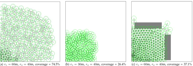
In the experiments, a total of 240 sensors are initially randomly distributed in a sub-area {(x, y) : 0 ≤ x ≤ 500m, 0 ≤ y ≤ 500m} of a target field {(x, y) : 0 ≤ x ≤ 1000m, 0 ≤ y ≤ 1000m}; the base station is located at (0, 0). Sensors have rc and rs varying between 30-60m;
they first move to gain connectivity, and then adjust their positions to maximize network coverage. The maximum moving speed is 2m/s, and the period length is 1 sec-ond; the simulation runs for 750 seconds, after which the sensor layout becomes quite stable. We define the metric coverage as the fraction of area that is covered by at least one sensor. In the first scenario (Figure 3(a)), sensors have rc = 60m and rs = 40m and move in an
obstacle-free field. It can be seen that CPVF distributes the sensors quite evenly, producing a coverage of 78.8%. When rc reduces to 30m (Figure 3(b)), the situation is
very different: the smaller rc makes the sensors cluster
together, producing a much smaller coverage of 28.7%. We can see that significant overlap of sensing disks (depicted by the circles) exists in the network, yet most sensors are unaware of this due to their poor ability to contact the sensors in their vicinities. Although the connected network provides the possibility for a sensor to find those whose sensing disks overlap with its own, the geography-based search is a non-local process and requires extra support from the protocol. Even if they can manage to make contact, significant coordination among many sensors may be needed to achieve an agreement
of movement that leads to a good layout. The impact of poor coordination is further demonstrated by the poor coverage (37.8%) in Figure 3(c), where rc = 60m, the
same as in Figure 3(a), but two rectangular obstacles are now present in the field, leaving three exits to the large vacant area. It turns out that the sensors have consider-able difficulty circumventing the obstacles: while a few can make their way out of the two top exits, no sensors can escape from the narrower exit at the bottom of the field. Increasing the run time does not help the sensors disperse: many of them only oscillate infinitely around their centers without being able to expand coverage.
4.4 Convergence of CPVF
During the experiments, we have observed another problem with CPVF: that the sensor layout does not converge easily. For many sensors, after a certain point in time, they start moving in a near cyclic way, without being able to move forward or stabilize. This problem is especially serious in a field with obstacles that form narrow or bumpy passages. The reason behind this is that every sensor makes movement decisions based only on the information of its neighbors. While the neighbor-hood changes, a sensor has to move; its move results in further change to the neighborhood, which forces other sensors to move – the constant change of virtual forces imposed on each sensor thus causes the sensors to move indefinitely.
A similar observation has also been made by Koren et al. [8]. In particular, they point out that oscillation happens very often in an irregular field which will significantly increase the overhead in terms of moving distance. We discuss this issue in Section 6.
In conclusion, while the VF-based approach has often been adopted in the planning of robotic movement and in mobile sensor deployment [14] [21] [9] [12], our ex-periments suggest that under the connectivity constraint, it delivers good performance only in very restrictive scenarios; an ideal field model as in Figure 3(a) thus conceals its drawbacks. These facts suggest that it is difficult, if not impossible, to remedy the VF method’s weaknesses without significantly compromising its lo-calized communication, which is the very reason for its popularity. This motivates us to look for alternative ways to improve the performance of a deployment scheme.
5
T
HE FLOOR-
BASED SCHEMEIn the CPVF method, the sensors move in a greedy fash-ion to establish connectivity; this can result in arbitrary overlaps of the sensors’ sensing ranges. When rc/rs is
small, the sensors lack information that can guide them to move apart in a coverage-maximizing way. A common situation is depicted in Figure 4(a), where the large circles represent sensing ranges, and the small circles represent communication ranges; rc/rsis assumed to be
0.5. It can be seen that despite the significant overlap of sensing ranges between the two groups (green and
(a) rc= 60m, rs= 40m, coverage = 74.5% (b) rc= 30m, rs= 40m, coverage = 26.4% (c) rc= 60m, rs= 40m, coverage = 37.1% Fig. 3. Sensor layouts under CPVF for varying rc andrs. The green circles represent sensors’ sensing ranges. The
1000 × 1000m2field is obstacle-free in (a) and (b), and has two obstacles in (c), shown as grey areas. There are 240 sensors that can move at a speed of no greater than 2m/s, with a period length of one second.
(a) CPVF (b) FLOOR floor line floor line (0,0) 2rs inter-floor line rc rs
Fig. 4. Examples of sensor layout under CPVF and FLOOR. The large circles represent sensing ranges, and the small circles represent communication ranges; rc/rs= 0.5.
yellow) of sensors, these sensors are unaware of this because of their short communication ranges.
The key idea of our floor-based method is to divide the field into floors of common height 2rs, and to encourage
sensors to stay at the central floor lines of those floors, as shown in Figure 4(b). Now that sensors are separated by floors, the overlap of the sensing ranges is much reduced, and so the global network coverage can be improved.
5.1 A high-level view
In FLOOR, sensors move in two patterns that bear a resemblance to the growth of a plant from the Vitis genus (e.g., a common vine) over a framework. The framework is composed of field/obstacle boundary lines and floor lines. In the first instance, nodes may expand along the field/obstacle boundaries, following possibly irregular paths; in the second instance, nodes may expand along the straight floor lines. If the floor lines are appropriately spaced, then beginning at some root, we would expect that using these two techniques good coverage will eventually be attained.
floor-line guided expansion
boundary guided expansion
Fig. 5. Coverage expansion in a field. The grey areas represent obstacles.rc= rs.
Figure 5 illustrates the two expansion patterns in a field with two irregular obstacles. The arrows show the directions in which sensors move along the boundary or floor lines. In the formal description, the first pat-tern is termed boundary-guided expansion, and the second pattern floor-line-guided expansion. These two patterns are performed in parallel. The first pattern is responsible for introducing sensors to the front end of every floor, while the second pattern is responsible for filling in the floors. We can expect that if enough sensor nodes are provided, then the field in Figure 5 will eventually be well covered. Moreover, the sensing overlap will be small due to the floor lines. The floor-based scheme is implemented in three phases:
1) achieving connectivity,
2) identifying movable sensors, and 3) expanding coverage.
In the first phase, sensors move toward the reference point to establish connectivity, following a different tra-jectory from that in CPVF for the sake of sensing overlap reduction. In the second phase, a class of nodes termed the fixed nodes are determined, and the remaining nodes,
termed the movable nodes, are provided the freedom to relocate for coverage expansion (from high-density to low-density areas). In the third phase, movable nodes expand their coverage following the expansion patterns introduced above.
5.2 Achieving connectivity
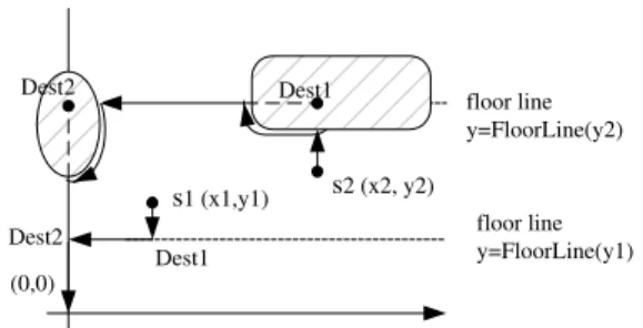
In this phase, a sensor does not move toward the base station in a straight line, as is the case in CPVF. Instead it is required to pass through two intermediate destinations. Suppose the initial location of the sensor is (x, y), then it first moves toward point D1, the projection point of (x, y) on its nearest floor line, using the BUG2 motion planning algorithm. Upon reaching D1 or hitting some obstacle, it takes D1 as a new starting point, and starts moving toward point D2, the projection of D1on the y axis. Upon reaching D2(or on collision with an object), the sensor takes D2 as a new starting point and begins moving toward (0, 0). During the algorithm, the lazy movement strategy is used, and the sensor stops once it enters the communication range of a connected node, which then becomes its parent. Note that in FLOOR, the distance between a sensor and its parent is min(rc, 2rs), and the y
axis is regarded as a wall-like obstacle. A more formal description of the above process is given in Algorithm 1.
Algorithm 1: FLOOR’s motion planning algorithm. input : Current location (x, y) and a connected field
with unknow topology
symbols:FloorLine(y): the y coordinate of the nearest floor line to the point (x, y)
start← (x, y);
1
target← (x,FloorLine(y));
2
Execute BUG2(start,target)until becoming connected, or 3
reachingtarget, or hitting an obstacle. If connected then terminate the algorithm;
start← (x,FloorLine(y));
4
target← (0,FloorLine(y));
5
Execute BUG2(start,target)until becoming connected, or 6
reachingtarget, or hitting an obstacle. If connected then terminate the algorithm;
start← (0,FloorLine(y));
7
target← (0, 0);
8
Execute BUG2(start,target)until becoming connected, or 9
reachingtarget.
In Figure 6, sensor s1 moves to (0, 0) after changing direction twice and without encountering any obstacles; sensor s2 meets two obstacles, thus preventing it from reaching the locations Dest1 and Dest2. By following Algorithm 1, it finally reaches location (0, 0).
5.3 Identifying movable sensors
After a sensor becomes connected, it reports to the base station, and waits for a response from the base station. The response message will reach the sensor carrying the IDs of all the sensor’s ancestors, which will be kept in the sensor’s memory. The base station initiates the second
(0,0) floor line y=FloorLine(y1) Dest2 s1 (x1,y1) s2 (x2, y2) floor line y=FloorLine(y2) Dest1 Dest2 Dest1
Fig. 6. Sensors’ moving paths toward (0, 0) under FLOOR.
phase after all sensors have reported their arrival, or after a certain time (e.g., an estimate of the maximum time for a sensor to arrive at the base station) has elapsed, whichever is earlier.
The purpose of the second phase is to identify sensors that can move without partitioning the network, and whose move is expected to increase network coverage. The former condition requires a sensor to help all of its children to find new parents. This can be done as follows. It first obtains a list of neighbors within two hops of itself, and then tries to find for each child a new parent. For a particular child, it needs to check if the child joining some candidate parent will cause a loop, which can be done by simply checking the candidate parent’s ancestor list. If all the children can find parents without creating loops, then it means that the sensor can safely move away. To become movable, a sensor also needs to decide whether its move is worthwhile in terms of coverage: it estimates the area currently covered exclusively by itself using the location information of its neighbors; only when such an area is below a certain threshold does it become movable.
To ensure state consistency, the procedure of identi-fying movable sensors needs to be serialized. This can be coordinated by a message traversing the tree in, for example, a depth-first manner. Such a message can be initiated by the base station at the start of this phase.
5.4 Determining the coverage status of a point
A sensor often needs to determine whether a point in its vicinity is covered by others, so that it can decide whether it needs to invite some movable sensor to fill that uncovered area. As demonstrated earlier, local com-munication is inherently limited in its ability to detect the coverage status of a point beyond a sensor’s sensing range, especially when rc/rsis small; thus some method
of non-local communication is inevitable.
With the field divided into floors, we are able to implement a simple scheme that solves this problem. We define a floor header node as the node with the smallest x-coordinate in a floor. (Ties can be resolved using the nodes’ IDs.) Each floor header node maintains a data structure that records the locations of the nodes in its floor. Since many fixed nodes are linked with the same
(or approximately the same) inter-node intervals, and thus share the same y-coordinate (i.e., they reside on the same floor line), their locations can be summarized in a compact form: given a sequence of such nodes, only the first and the last nodes’ x-coordinates need to be recorded. For instance, in the layout shown in Figure 8(a), the floor header nodes need to record only a small amount of information concerning the nodes locations on their floor lines. When a node s needs to determine whether a point p beyond its sensing range is already covered, it firsts checks whether any of its neighbors covers that point; if not, it then calculates the possible floors that may contain a node whose sensing range can reach p. s then sends a query message to the floor header nodes corresponding to those floors. Those floor header nodes can in turn determine whether p is covered by any sensor in their own floors, and send back their responses, from which s can determine p’s coverage status. Note that this task need not be done with perfect accuracy, since strict performance optimality is not our goal.
Every node in the tree records the floor header nodes in the sub-tree rooted at itself, so the query messages can be easily routed on the tree. Given a field of fixed width and a fixed rc, there will be a constant number of
floor header nodes, therefore the memory overhead will be bounded.
5.5 Expanding sensing coverage
With all movable sensors identified, we can now ex-pand the network’s coverage by having those sensors move to uncovered areas. In Section 5.1 we provide a high-level description for floor line guided expansion (FLG-expansion) and boundary line guided expansion (BLG-expansion). We will also describe a third type of expansion, termed inter-floor line guided expansion (IFLG-expansion).
For each type of operation, a sensor first needs to find an expansion point (EP) on its expansion circle, defined as the circle of radius min(rc, rs) centered at its current
location, after which it invites some movable sensor to relocate to the EP. When searching for expansion points, we only consider the environment consisting of fixed nodes. A formal description of this process is given in Algorithm 2.
5.5.1 Finding expansion points
• FLG-expansion. A sensor s tries to obtain a floor
line segment covered by its sensing range (see Figure 7(a)). If such a segment exists, it picks one endpoint of that line segment that is farthest to the y-axis. Such a point is called a frontier point. Next, s determines whether that frontier point is covered by other sensors using the method introduced in Section 5.4. If s can find an uncovered frointer point, it calculates the intersection between its expansion circle and the line segment from s’s current location
B C O (a) (d) (b) inter-floor line floor line A B C A O (c) (a) C A B O floor line A'
Fig. 7. Illustration of coverage expansion. (a, b, c) BLG-and FLG-expansion; (d) IFLG-expansion. The grey irreg-ular areas represent obstacles.rc= rs.
to the frontier point; the intersection point is the desired EP.
• BLG-expansion. A sensor s tries to obtain a set
of boundary line segments covered by its sensing range (see Figure 7(a)). If any such line segments ex-ist, it randomly picks a segment, say Γ, and chooses a random point on Γ and moves the point along Γ following the left-hand rule1, until the point reaches the sensing circle; this new location is the frontier point for Γ. After determining the frontier point, s calculates the EP following the same procedure as in the FLG-expansion.
• IFLG-expansion. This type of expansion is used for
filling coverage holes left by neighboring sensors in the same floor (see Figure 7(d)). A sensor and its child can jointly determine if there is a coverage hole between themselves and an inter-floor line, which is defined as that at the middle of two neighboring floor lines. If a hole is found, then the parent checks if the intersection point of their expansion circle at the side of the hole is already covered by other sensors. If it is not, then the intersection point is taken as an EP.
With an EP determined, s can start inviting movable sensors over. After a movable sensor has agreed to such a move, the above process is repeated. Figure 7 illustrates the three types of expansion. In Figure 7(a), the sensor centered at O detects three line/curve segments (the thick lines) in its sensing range: one from the floor line, and two from the two obstacles. Using the left-hand rule, it can obtain three frontier points, A, B, and C. Suppose s has just discovered that A is uncovered, it then takes
1. The left-hand rule, as opposed to the right-hand rule used by the sensors to establish connectivity, can help sensors disperse into unexplored areas more quickly.
A as an EP and invites a movable sensor to relocate to it, resulting in the layout shown in Figure 7(b). Afterwards, s can continue to find movable sensors to relocate to B and C. At the same time, the newly arriving sensor centered at A can determine its own EP A0 and invite
sensors to move to that EP; see Figure 7(c). An example of IFLG-expansion is provided in Figure 7(d).
Algorithm 2: Coverage expansion.
———- Pseudo-code of fixed node thread 1 (discovering EPs) 1
while there exists at least one EP do
2
Let p be one of the EPs; 3
Send a random-walkInvitationmessage carrying 4
the location and type of p, along with a TTL;
end
5
———- Pseudo-code of fixed node thread 2 (handling messages) 6
while true do
7
Wait for a message m to come through; 8
p ← the EP that m corresponds to; 9
msrc← the source node of m
10
if p is covered by a fixed or virtually fixed node then
11
Send arejectmessage to msrc;
12
else
13
Send anAcknowledgemessage to msrc;
14
Construct a virtual fixed node for msrc;
15
Send a message to the root on behalf of the virtual 16
node to update the ancestors’ location information;
end
17
end
18
———- Pseudo-code of movable node 19
while true do
20
Wait until having collected a certain number of 21
Invitationmessages, at the same time forwarding
received random-walk messages;
Pick the highest-priority message m (and smallest 22
Euclidean distance when ties occur), with source msrc;
Send anAcceptInvitationmessage back to msrc;
23
Wait for anAcknowledgemessage with a timeout; 24
if anAcknowledgemessage is accepted then 25
Move to the EP contained in m following BUG2; 26
Mark itself to be fixed; 27 Exit; 28 end 29 end 30
Generally, FLG-expansion provides more
improvement in coverage per operation, so it is assigned the highest priority in the protocol; BLG-expansion is ranked second, and IFLG-BLG-expansion has the lowest priority.
5.5.2 Inviting movable sensors
The sensors check the sensing coverage and obstacles in their surrounding areas once per period, and determine whether there is any chance for expansion. If a sensor finds no expansion points on its expansion circle, then it stops the checking process. Otherwise, it sends an
Invitationmessage containing an EP to the network.
This message has a TTL value and walks randomly in the network. When a movable sensor has collected a certain number of invitations, it picks the one with the highest priority (and smallest Euclidean distance when ties occur). It then sends an AcceptInvitation
message to the inviter, which acknowledges the message if it has not found any other movable sensor for that EP, or rejects it otherwise. In the former case, the movable sensor can start to relocate; at the same time the inviting sensor constructs a virtual place-holding fixed node in the tree, and sends a message to the root on behalf of the invited sensor to update the location information maintained by its ancestors. If theAcceptInvitation
message is rejected or no response has been received, the movable sensor simply continues to collectInvitation
messages and responds to an inviter when appropriate. Once a movable sensor moves to an EP, it becomes fixed and can start searching for expansion opportunities around itself. It is possible that two movable sensors re-locate to the same (or very near) positions, thus wasting coverage. However, the chance of such an occurrence will be small as long as the communication latency is much smaller than the length of a period. The wasted coverage is thus insignificant.
5.6 Coverage of FLOOR
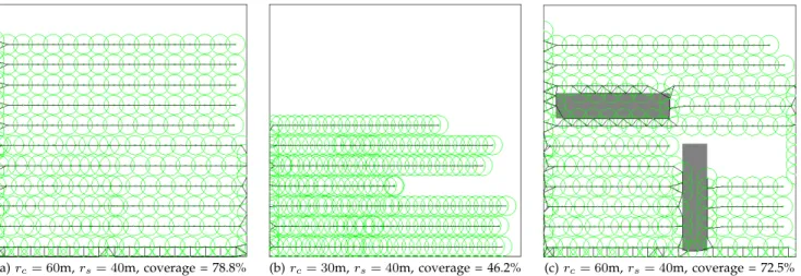
We conduct simulations for FLOOR using exactly the same settings as in Figure 3, and show the sensor layout in Figure 8. When the field is obstacle-free (Figure 8(a)), the coverage achieved by FLOOR is 78.8%, which is slightly higher than that of CPVF (74.5%). When rc
decreases to 30m (Figure 8(b)), FLOOR produces a much higher coverage than CPVF (46.2% vs. 26.4%). This is because FLOOR can separate sensors using floor lines, thus reducing coverage overlap in the vertical direction to minimum. This example clearly demonstrates the advantage of FLOOR over CPVF in adapting to varying rc. Another advantage of FLOOR can be seen from
Fig-ure 8(c), where two obstacles are present in the field. In contrast to CPVF, FLOOR has no difficulty expanding the coverage beyond those obstacles, producing a coverage of 72.5%, nearly twice that of CPVF.
In FLOOR, once a movable sensor relocates to a certain location it stabilizes, and so the convergence time of the protocol is bounded.
6
COMPREHENSIVE PERFORMANCE
EVALUA-TION
In this section we conduct a more comprehensive per-formance evaluation of the proposed schemes. Besides coverage, we also consider the moving distance of sen-sors, which dominates energy consumption in the de-ployment process. A further energy consumption fac-tor that we investigate is the message overhead. The same settings of field, sensor movement patterns, and the ranges of rc and rs as in Section 4.3 are used.
We consider a clustered initial sensor distribution, in which sensors are randomly distributed in a sub-area {(x, y) : 0 ≤ x ≤ 500, 0 ≤ y ≤ 500} of the whole field {(x, y) : 0 ≤ x ≤ 1000, 0 ≤ y ≤ 1000}. This distribution is intended to test how sensors move apart from a clustered
(a) rc= 60m, rs= 40m, coverage = 78.8% (b) rc= 30m, rs= 40m, coverage = 46.2% (c) rc= 60m, rs= 40m, coverage = 72.5% Fig. 8. Sensor layout using FLOOR for varyingrc and sensing rangesrs. The field is obstacle-free in (a) and (b), and
has two obstacles in (c), shown in grey.
distribution to maximize network coverage. We have also tested an initial distribution in which sensors are placed in the field uniformly at random; the results are consistent with the clustered case, so we mainly report on the former.
6.1 Coverage in obstacle-free fields
Assuming an obstacle-free field, we compare the cover-age performance of five schemes:
1) CPVF, described in Section 4; 2) FLOOR, described in Section 5;
3) The optimal scheme (OPT) described in [1]. This centralized scheme achieves provably optimal cov-erage with guaranteed connectivity (applicable only to obstacle-free regular fields);
4) VOR, an Voronoi Diagram (VD) based scheme, in-troduced in [14]. In VOR, nodes move in rounds; in each round, every node moves toward its farthest Voronoi polygon vertex, under the constraint of a maximum moving distance of rc/2;
5) Minimax, also an VD-based scheme, introduced in [14]. Like VOR, nodes move in rounds; in each round, every node moves to the point that has the smallest distance to its farthest Voronoi polygon vertex.
These schemes include state-of-the-art techniques for our deployment task: CPVF represents the VF-based approach, while VOR and Minimax represent the VD-based approach. (In [14] the authors also propose a third scheme but since it performs no better than VOR and Minimax we ignore this case.) Note that VOR and Minimax are connectivity-ignorant.
6.1.1 Comparison between CPVF, FLOOR and OPT Figure 9 shows the coverage of CPVF and FLOOR for varying numbers of sensors. The results confirm previ-ous findings from Figures 3 and 8: FLOOR outperforms CPVF in all cases, especially for a moderate or small rc/rs. For instance, for 240 sensors with rc = 20m
and rs = 60m, the coverage of CPVF (20%) is only
46% of FLOOR’s coverage (46%). As rc/rs increases,
the gap becomes smaller. For example, with rc = 60m
and rs = 20m, the coverage of CPVF and FLOOR are
24% and 28%, respectively (not shown in the figure). Generally, in an obstacle-free field, when rc ¿ rs, the
advantage of FLOOR is most pronounced; when rc À rs,
the two schemes come very close in coverage.
Figure 9 also plots the results of OPT. As can be seen, FLOOR is only surpassed by OPT by a small to moderate margin, with the largest difference occurring at rc = rs = 60 with 120 sensors, where the coverage
of FLOOR is 26% lower than the optimal. As rc and the
number of sensors grows, FLOOR’s coverage becomes quite close to the optimal. For instance, for rc= rs= 60
with more than 200 sensors, FLOOR’s coverage is only 4% lower than the optimal. Further increase of sensors (≥ 300) brings diminishing gains in coverage as the field gradually becomes saturated (expect under the case of CPVF with rc = 40m and rs= 60m).
The difference between FLOOR and OPT is mainly due to some sensors that are located at the boundary of the field. Here the coverage holes are smaller than those found at the interior of the field, and therefore the coverage gains are smaller than average. In a system where a central coordinator is absent, achieving a perfect (and strict) pattern will require more sensor relocations, which leads to increased energy consumption. It is FLOOR’s choice to trade a small amount of coverage for a saving in energy consumption. This point will be further demonstrated in the next section.
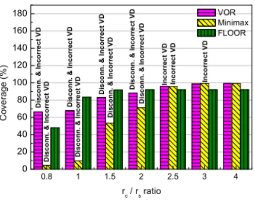
6.1.2 Comparison between FLOOR, VOR and Minimax In a VD-based scheme, the connectivity and coverage prove to highly depend on rc/rs. Figure 10 compares the
coverage of the three schemes for rs = 60 and rc/rs ∈
[0.8, 4]. Above the bars, labels “Disconn.” and “Incorrect VD” indicate network disconnection and the failure to generate all correct VD cells, respectively. One can make several observations from this figure:
Fig. 9. Coverage of CPVF, FLOOR, and OPT.
Fig. 10. Coverage of CPVF, VOR, and Minimax,rs= 60.
• Neither VOR nor Minimax achieves connectivity for
rc/rs≤ 2, which suggests they rely on a large rc/rs
to generate a fully functional network; nevertheless, even if rc/rs is large, there is no guarantee of
con-nectivity from the principle of VOR and Minimax;
• VOR and Minimax start generating correct VD cells
only when rc/rs≥ 3 and rc/rs≥ 4, respectively. The
improving coverage with increasing rc/rs implies
the significant impact of correct VD generation on coverage performance. In particular, the Minimax scheme is extremely sensitive to rc/rs: when the
ratio is smaller than 1, the resulting network is very unreasonably deployed, producing a coverage of only 4.5%;
• If rc/rsis large enough (≥ 2.5 in our case), both VOR
and Minimax perform well in terms of coverage. In some cases, they are very close to the optimal and slightly outperform FLOOR. The reason is that they do not consider connectivity and thus have more freedom for coverage maximization.
6.2 Moving distance in obstacle-free fields
We compare the moving distance of sensors for six schemes, including CPVF, FLOOR, VOR, Minimax, and two other schemes.
Fig. 11. Average moving distance.
Fig. 12. Effect of oscillation avoidance on moving dis-tance (left y-axis) and coverage (right y-axis).
When the sensors are initially densely deployed within a sub-area of the field, as is the case for our first distri-bution setting, VOR and Minimax need an “explosion” procedure to disperse the sensors into an approximately random distribution, and then VD-based coverage im-provement can begin. We let this stage take a minimum total moving distance, which can be calculated as fol-lows. We assume that the resulting random distribution is already known, then choosing a destination point in this distribution for each sensor can be modelled as a classic minimum weighted bipartite matching problem (or an assignment problem), where the objective is to find the assignment that requires the minimum matching cost. This problem can be solved in polynomial time using the well-known Hungarian algorithm [7]. Calculating a minimum value for VOR and Minimax gives us a base-line as to how they perform in terms of moving distance in the best case. After the initial explosion process, we let VOR and Minimax run for 10 rounds, after which the coverage stabilizes.
Using the Hungarian algorithm, we also implement two optimal schemes with respect to two final network layouts. The first network layout is the optimal pattern
proposed in [1], and the second is the one produced by FLOOR itself. The first optimal scheme shows the minimum moving distance for achieving an optimal coverage, while the second scheme shows how much FLOOR deviates from the lower bound with its own coverage.
Figure 11 shows the average moving distance of these six scheme. Comparing FLOOR with VOR and Minimax, one can see that FLOOR performs significantly better. The main source for VOR and Minimax’s long moving distance is the explosion process, despite the optimized moving arrangement. Without this process, VOR and Minimax will suffer from the same problems as VF-based scheme: a long convergence time and motion oscillation. This reflects VOR and Minimax’s reliance on a good initial sensor distribution.
Comparing FLOOR with the optimal schemes, one can also see that the moving distance of FLOOR is lower than that required by the optimal pattern. This is so because when planning node movement, FLOOR takes a more comprehensive consideration of coverage and moving distance – if a sensor finds that its move brings only a small gain in coverage, then the sensor remains fixed. Although sacrificing a certain amount of coverage, this strategy can effectively reduce the moving distance. In contrast, the optimal pattern only consid-ers total coverage, thus potentially involves more node movement. These results again demonstrate FLOOR’s choice in striking a balance between maximum coverage and minimum energy consumption.
It can also be observed that FLOOR has a moving distance 15.6-38% higher than the optimal for achieving its own coverage. This is no surprise since in FLOOR, the matching between coverage holes and movable sensors is performed in a distributed and greedy manner.
Comparing FLOOR with CPVF, one can see that CPVF generally requires more than two times the average moving distance of FLOOR. The reason behind this is that frequent oscillation occurs in CPVF, that is, many sensors move back and forth under the drive of virtual forces, requiring a large number of unnecessary moves on the way to their destinations.
The disadvantage of CPVF in terms of moving dis-tance is also found in the case where sensors are ini-tially distributed uniformly at random. Although it is the case that when connectivity is established, FLOOR requires all the sensors to try to pass two intermediate destinations, which causes more movement compared with CPVF’s straight-line movement, the oscillation of CPVF in the coverage maximization phase cancels out this advantage and leads to increased moving distance.
6.3 Oscillation avoidance for CPVF
We consider two oscillation avoidance techniques for reducing unnecessary movement in CPVF, in an attempt to remedy its drawbacks while retaining its strengths. In the first technique, called one-step oscillation avoidance, a
sensor cancels its movement for the next step if it finds that the next step size is smaller than V T /δ, where V T is the maximum step size and δ is a parameter called the oscillation avoidance factor. This is intended to eliminate small perturbations and force the system to enter an equilibrium state earlier; see [6] for a similar strategy. In the second technique, called two-step oscillation avoidance, a sensor compares its future location at the end of the next step with its past location at the end of the previous step; if the distance between them is smaller than V T /δ, then it cancels its movement plan for the next step. A similar approach has been used in [14]. Figure 12 shows the impact of varying the δ value on the moving distance (the left y-axis) and coverage (the right y-axis) of both schemes. It can be observed that δ does have the effect of reducing the moving distance; however, this comes at the cost of reduced coverage. When δ gets smaller, it is more likely that a step will be regarded as an unnecessary or repeated move, thus more steps are cancelled. On the other hand, the conservative moving of sensors prevents them from exploring the uncovered areas effectively, resulting in poor coverage. We have also tried oscillation avoidance based on a longer movement history, and have found similar trends. The difficulty of avoiding oscillation without reducing coverage is that some seemingly unnecessary steps are actually effective moves that can potentially push the frontier of coverage forward, yet it is very hard to detect which of these moves are effective, so that we can decide when to start the oscillation avoidance and when to stop it. The failure of reducing oscillations by local decisions again reflects the limitation of the VF-based approach.
6.4 Fields with random obstacles
We next consider sensor deployment in a field with obstacles. In this setting, the previously discussed op-timal and VD-based schemes no longer apply, so we only consider CPVF and FLOOR. We randomly select between 1 and 4 rectangular obstacles of random size; these obstacles may overlap with one another, however we maintain the condition that the obstacles do not partition the field.
A total of 300 runs of the simulation are executed, and the coverage and moving distance of the two schemes are recorded. Figure 13 depicts the cumulative distri-bution function of coverage and average distance. In this general obstacle setting, it can be seen that FLOOR outperforms CPVF significantly in terms of both cover-age and moving distance. For instance, while the mean coverage of FLOOR is more than 20% higher than that of CPVF, the mean moving distance is less than half that of CPVF.
6.5 Message overhead
We examine the message overheads of FLOOR by vary-ing the TTL values used in the sensor invitation process, and recording the number of protocol messages that are
(a) CDFs of coverage
(b) CDFs of moving distance
Fig. 13. Comparison of CPVF and FLOOR in coverage and moving distance under random obstacles.
transmitted during the simulation. Table 1 shows the total (and average) number (×1000) of protocol messages for varying numbers of sensor nodes N , and T T L as a fraction of N , under the non-obstacle environment, as well as the two-obstacle environment as shown in Figure 3(c).
We can see that the per-node message overhead during the 750 seconds is quite moderate. For instance, for N = 200 and T T L = 0.2 × N = 40, the overhead is 3.1 × 1000 = 3100 messages per node, which translates to approximately 4 messages per node per second. These messages are all short query messages. This is unlikely to be a high bandwidth requirement for current sen-sor hardware. When the network grows, more message transmissions will be incurred. In this case, the periods could be prolonged to guarantee that the bandwidth requirement does not exceed the limit of sensor nodes.
It should be noted that the energy consumption for message transmissions is usually very small compared with the energy consumption required for mechanical movement. Besides, the deployment process is often very short in comparison with the expected network lifetime (e.g., hours vs. weeks). We thus believe that the message overhead of FLOOR is acceptable for many of today’s applications. T T L as a fraction of N 0.1N 0.2N 0.3N 0.4N non-obstacle environment N = 120 225 (1.9) 306 (2.6) 388 (3.2) 470 (3.9) N = 160 325 (2.0) 472 (3.0) 620 (3.9) 769 (4.8) N = 200 409 (2.0) 623 (3.1) 837 (4.2) 1052 (5.3) N = 240 457 (1.9) 714 (2.9) 970 (4.0) 1228 (5.1) two-obstacle environment N = 120 198 (1.7) 286 (2.4) 372 (3.1) 460 (3.8) N = 160 296 (1.8) 453 (2.8) 609 (3.8) 767 (4.8) N = 200 387 (1.9) 617 (3.1) 846 (4.2) 1077 (5.4) N = 240 428 (1.8) 700 (2.9) 973 (4.1) 1246 (5.2) TABLE 1
Total(/average) number (×1000) of protocol messages required by FLOOR during a 750-second period.
7
C
ONCLUSION AND FUTURE WORKWe have presented two sensor deployment schemes for mobile sensor networks in general 2-D fields. The major difference of our schemes from previous work is their adaptability to arbitrary network densities or com-munication ranges, and to obstacles. Our first scheme is an enhanced form of the traditional virtual force-based method. We show that it performs well only in very restricted scenarios. We then consider a floor-based scheme which shows good performance in all cases. As part of our future research we plan to investigate how to extend these schemes from deployment through to the whole life cycle of a mobile sensor network – including tasks such as failure recovery and balancing movement overhead. A higher degree of coverage/connectivity in dense networks will also be considered.
R
EFERENCES[1] X. Bai, S. Kumary, D. Xuan, Z. Yun, and T. H. Lai. Deploying Wireless Sensors to Achieve Both Coverage and Connectivity.
Proc. of MobiHoc’06. Italy, 2006.
[2] X. Bai, Z. Yun, D. Xuan, T. H. Lai, and W. Jia. Deploying Four-Connectivity And Full-Coverage Wireless Sensor Networks. Proc.
of INFOCOM 2008.
[3] W. Cheng, M. Li, K. Liu, Y. Liu, X-Y Li, and X. Liao. Sweep Cov-erage with Mobile Sensors. In Proc. of the 22nd IEEE International
Parallel and Distributed Processing Symposium (IEEE IPDPS), Miami,
Florida, USA, April 2008.
[4] J. Cortes, S. Martinez, T. Karatas, and F. Bullo. Coverage control for mobile sensing networks. IEEE Transactions on Robotics and
Automation 20 (2), 243-255, 2004.
[5] N. Heo and P. K. Varshney. Energy-Efficient Deployment of Intelligent Mobile Sensor Networks. IEEE Transactions on Systems,
Man, and Cybernetics – Part A: Systems and Humans, 35(1):78-92,
Jan. 2005.
[6] A. Howard, M. J Mataric, and G. S. Sukhatme. Mobile Sensor Network Deployment using Potential Fields: A Distributed, Scal-able Solution to the Area Coverage Problem. In Proc. of the 6th
International Symposium on Distributed Autonomous Robotics Systems (DARS02), 2002.
[7] Hungarian Algorithm.
http://en.wikipedia.org/wiki/Hungarian_algorithm
[8] Y. Koren and J. Borenstein. Potential Field Methods and Their Inherent Limitations for Mobile Robot Navigation. In Proc. of the
IEEE Conference on Robotics and Automation. California, USA. 1991.
[9] J. Lee, A. D. Dharne, and S. Jayasuriya. Potential Field Based Hierarchical Structure for Mobile Sensor Network Deployment. In Proc of the 2007 American Control Conference. New York City, USA, 2007.
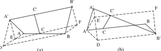
A B A' B' C' C D E B A A' B' C' C E D (a) (b) F F
Fig. 14. Moving paths of two sensorssands0. In (a),s’s
path ABands0’s path A0B0 do not intersect; in (b), their
paths intersect at some point.
[10] B. Liu, P. Brass, and O. Dousse. Mobility Improves Coverage of Sensor Networks. In Proc. of ACM MobiHoc, 2005.
[11] V. J. Lumelsky and A. A. Stepanov. Path-planning strategies for a point mobile automaton moving amidst unknown obstacles of arbitrary shap. Algorithmica, 2:403-430, 1987.
[12] S. Poduri and G. S. Sukhatme. Constrained Coverage for Mobile Sensor Networks. Proc of International Conference on Robotics and
Automation. New Orleans, 2004.
[13] G. Wang, G. Cao, T. L. Porta, and W. Zhang. Sensor Relocation in Mobile Sensor Networks. Proc. of IEEE INFOCOM’05.
[14] G. Wang, G. Cao, and T. L. Porta. Movement-Assisted Sensor Deployment. Proc. of IEEE INFOCOM’04, Hong Kong, 2004. [15] G. Wang, G. Cao, and T. L. Porta. A Bidding Protocol for Sensor
Deployment. Proc. of the IEEE ICNP, Georgia, USA. 2003. [16] W. Wang, V. Srinivasan and K.-C. Chua. Trade-offs Between
Mobility and Density for Coverage in Wireless Sensor Networks. In ACM Proc. of MobiCom 2007.
[17] G. Xing, X. Wang, Y. Zhang, C. Lu, R. Pless, and C. Gill. Integrated Coverage and Connectivity Configuration in Wireless Sensor Networks. ACM Transactions on Sensor Networks. 1(1):36-72, 2005. [18] S. Yang, M. Li, and J. Wu. Scan-Based Movement-Assisted Sensor Deployment Methods in Wireless Sensor Networks. IEEE
Trans-actions on Parallel and Distributed Systems (TPDS), 2006.
[19] O. Younis, M. Krunz, and S. Ramasubramanian. Coverage With-out Location Information. Proc. of IEEE ICNP 2007.
[20] J. Zhao and R. Govindan. Understanding Packet Delivery Per-formance in Dense Wireless Sensor Networks. In Proc. of ACM
Conference on Ebmedded Networked Sensor Systems (SenSys), pages
1-13, Los Angeles, CA, 2003.
[21] Y. Zou and K. Chakrabarty. Sensor Deployment and Target Lo-calization Based on Virtual Forces. Proc. of IEEE INFOCOM 2003.
APPENDIX
A
PROOF OF
CPVF
GUARANTEEINGCONNECTIV-ITY
We formally prove that CPVF guarantees connectivity throughout the process of VF-driven sensor movement. We assume that all sensors follow the connectivity pre-serving conditions, and that the message transmission latency is negligible compared with the length of a period.
Following the argument made in Section 4.2, we need to prove that for a sensor s planning for its next move and its neighbor s0, their distance will be no greater than
rc at any time during [t, t0], given that their distances at
time t and t0are both no greater than r
c. The paths of the
two sensors are illustrated in Figure 14, where the line segments AB and A0B0 represent s’s planned path and
s0’s moving path during [t, t0], respectively, and AA0≤ r c
and BB0 ≤ r
c. Geometrically, we need to prove that for
any point C on AB, and point C0 on A0B0, we satisfy
AC/AB = A0C0/A0B0, CC0≤ r c.
Now consider the case in Figure 14(a) where AB and A0B0 do not intersect. Draw line segment EC parallel
and equal to A0C0, and line segment CF parallel and
equal to C0B0; also draw line segment DB parallel and
equal to A0B0. Since DBkA0B0 and EF kA0B0, DBkEF ,
thus DEkBF . Because AC/AB = A0C0/A0B0 = EC/EF ,
we have EAkBF . Hence, EA and DE are on the same line.
Since A0B0BD is a parallelogram, we have A0D =
BB0; likewise A0E = CC0. As assumed, A0D ≤ r c
and A0A ≤ r
c; if A0E > rc, then 6 A0DE +6 A0AE > 6 A0ED +6 A0EA = 180◦, which is impossible. Therefore
A0E must be no greater than r
c, as is the case for CC0,
as desired.
The proof for the case in which AB intersects A0B0, as
shown in Figure 14(b), is similar to the above argument and is thus omitted.
PLACE PHOTO HERE
Guang Tan received the Bachelor’s degree from
the Chongqing University of Posts and Telecom-munications, China, in 1999, the Master’s de-gree from the Huazhong University of Science and Technology, China, in 2002 and the Ph.D. degree in computer science from the University of Warwick, U.K., in 2007. He is currently a postdoc researcher in the ASAP Group, French National Institute for Research in Computer Science and Control (INRIA), Rennes, France. From 2002 to 2004, he worked in industry as a software engineer. His area of interest is distributed systems and networks. He is a member of the IEEE.
PLACE PHOTO HERE
Stephen A. Jarvis is an associate professor and
the head of research in the Department of Com-puter Science, University of Warwick, U.K. While previously at the Oxford University Computing Laboratory, he worked on the development of performance tools with Oxford Parallel, Sychron Ltd., and Microsoft Research, Cambridge. He has close research ties with the industry, in-cluding current projects with IBM, BT, Hewlett-Packard Research Laboratories, and AWE. He has authored more than 120 refereed publica-tions (including three books) in the area of software and performance evaluation. He is also co-organizer for one of the UK’s high-end scientific computing training centers, the manager of the Midlands e-Science Technical Forum on Grid Technologies and a member of the EPSRC and BBSRC Peer Review Colleges. He is member of the IEEE.
PLACE PHOTO HERE
Anne-Marie Kermarrec obtained her Ph.D.
from the University of Rennes in October 1996. She spent a year (Oct.96- Oct97) in the Com-puter Systems group of Vrije Universiteit, Ams-terdam. In 1997, she became an assistant pro-fessor at the University of Rennes. In 2000, she joined Microsoft Research in Cambridge and worked in the area of peer-to-peer computing. Since February 2004, she has been a senior researcher at INRIA, Rennes, France. Her re-search interests include large-scale distributed systems, peer to peer overlay networks and applications.