CAD-guided inspection of aeronautical mechanical parts using monocular vision

HAL Id: hal-01352472

https://hal.archives-ouvertes.fr/hal-01352472

Submitted on 8 Aug 2016

HAL is a multi-disciplinary open access

archive for the deposit and dissemination of

sci-entific research documents, whether they are

pub-lished or not. The documents may come from

teaching and research institutions in France or

abroad, or from public or private research centers.

L’archive ouverte pluridisciplinaire HAL, est

destinée au dépôt et à la diffusion de documents

scientifiques de niveau recherche, publiés ou non,

émanant des établissements d’enseignement et de

recherche français ou étrangers, des laboratoires

publics ou privés.

CAD-guided inspection of aeronautical mechanical parts

using monocular vision

Ilisio Viana, Florian Bugarin, Nicolas Cornille, Jean-José Orteu

To cite this version:

Ilisio Viana, Florian Bugarin, Nicolas Cornille, Jean-José Orteu. CAD-guided inspection of

aeronau-tical mechanical parts using monocular vision. 12th International Conference on Quality Control by

Artificial Vision (QCAV’2015), May 2015, Le Creusot, France. �10.1117/12.2182922�. �hal-01352472�

CAD-guided inspection of aeronautical mechanical parts

using monocular vision

Viana I.

, Bugarin F.

, Cornille N.

, Orteu J-J.

a

_Universit´

_{e de Toulouse ; INSA, UPS, Mines Albi, ISAE ; ICA (Institut Cl´}

_{ement Ader) ;}

Campus Jarlard, F-81013 Albi, France

b

_G

_{Metric, 40 Chemin Cazalbarbier, F-31140 Launaguet, France}

ABSTRACT

This paper focuses on quality control of mechanical parts in aeronautical context by using a single PTZ camera and the CAD model of the mechanical part. In our approach two attributed graphs are matched using a similar-ity function. The similarsimilar-ity scores are injected in the edges of a bipartite graph. A best-match-search procedure in bipartite graph guarantees the uniqueness of the match solution. The method achieves excellent performance in tests with synthetic data, including missing elements, displaced elements, size changes, and combination of these cases.

Keywords: Computer-Aided-Inspection, Image Analysis, Feature Matching, Graph Matching, PTZ camera

1. INTRODUCTION

For a company, checking products conformity is the guarantee to ensure good quality delivery for its consumers, to potentially save costs by avoiding products return and in crucial applications to prevent accidents. As a result, a lot of effort are continuously made by security organizations, industry and research institutions in order to improve quality control methodologies. Defect inspection using computer vision is a widely studied topic.1–4 _It is suitable for contactless inspection and it ensures uniform, consistent and quick defect control. In the primary days of inspection using camera information, black and white image of a non defective element was used as a reference which was compared with the tested and potentially defective element. Over the years different approaches have been used such as correlation of defect-free image with test image, contour comparison, and more sophisticated approaches such as comparison of a model representing the non defective element with the potentially defective element, as in.5, 6

In this paper we address the Computer-Aided-Inspection problem, trying to make sure the tested element is congruent with its CAD model. In our approach the reference is an image derived from a CAD model. This model contains primitives (including segments and ellipses) representing the element to be controlled. Our goal consists in comparing this theoretical image with a real acquired image. This type of approach was used in7 _to help in 3D reconstruction and in8_{for mechanical object alignment. Karabagli}9_{used theoretical versus real image} comparison to check machining set-up elements placement in a High-Speed-Machining application. This paper addresses the problem of mechanical assembly in aeronautical context under the constraint of robustness and flexibility. That means that we should be capable of detecting defects with a high level of assurance while being flexible enough regarding to false alarm detection in order not to discourage the end user. In all the mentioned works, contours were the information used. In some cases like,9 _{contours were associated with other types of} information (skeletons, geometric metrics...) In our work, we use mathematically characterized primitives. Our work belongs then to the group of geometry-based matching methods.

1111M-

fis

O O

o

2. SETUP:

PTZ CAMERA ASSOCIATED WITH DIRECTED LIGHT DEVICE

AND CAD MODEL

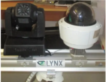
This section describes our CAD-guided inspection method set-up and how both real and CAD data are exploited in order to make acceptance / rejection decision. Our goal is to check a mechanical assembly made of several elements and whose CAD model is known, by processing only 2D data generated from CAD model on one hand and acquired image on the other hand. Our acquisition system is composed of a high definition Pan-Tilt-Zoom (PTZ) dome and one directional light device moving synchronously with the PTZ camera, cf. figure 1.

This acquisition system is provided by the company G2Metric who has developed an inspection software named

Figure 1: Acquisition system : PTZ camera and the directional light device

Lynx which carries out the inspection task by comparing an acquired image with a defect free reference image stored in a data base. Our goal using the CAD model is to work on a new version of Lynx in order to replace the reference image by an image derived from the CAD model. Data used during the inspection process are obtained through two different stages. At first, CAD-derived image is generated as a screenshot of our CAD model at one given position previously decided by the user as a representative view for the element to be controlled. From CAD model we coarsely estimate a look-up table for the pan and tilt parameters of our PTZ camera, also we estimate a congruent zoom factor for the PTZ camera in order to have the same scale for both theoretical and real element. Secondly, we use all this parameters to direct our acquisition system toward the element to be inspected. The inspection is guided by the CAD model. We select an element in the CAD model, we orient the PTZ camera toward the real element and we take an image of the element. In the end of this procedure we have a set made of theoretical and real images, cf. figure 2.

The hypothesis here is to consider that the parameters used to generate the theoretical image are sufficient to help us positioning the real camera in order to have two comparable images. In fact our main goal during this work is to be able to compare one theoretical image with one real image assuming that they are aligned. Even if

Figure 2: Set of images generated from CAD model (top) and real images acquired with PTZ camera (bottom) we assume that our images are aligned, comparing a theoretical image with a real image is a challenging because the first is created using mathematical object description and the second captures the object description using optics. In that sense, the first question to ask is what kind of information can be used to achieve a robust

comparison of these images. In the next section we describe our CAD-based matching method of an image generated from a CAD model with an image acquired with the PTZ camera.

3. METHOD:

CAD-BASED MATCHING OF PRIMITIVES FROM REAL AND

THEORETICAL IMAGES

In this section, we describe our method, starting with a short literature review in subsection 3.1. Subsection 3.2 describes the primitives used in the matching process and how they can be extracted from the images. The matching process is accomplished in three stages. In subsection 3.3 we compute a similarity function for each pair of theoretical and real primitive, the similarity scores are used in subsection 3.4 as edges weights of a bipartite graph which is optimized to keep only the best weighted edges. After the best match selection, in subsection 3.5 we construct two graphs, one for the best match candidates in the theoretical case and another one for the best matches in the real case. As the method is CAD-based, only the matches obeying to the neighbourhood criterion (distance/orientation) in both the real and the theoretical case are certified sure.

3.1 Related works

Matching is the task of finding correspondences between elements of data schemas or data instances.10 Match-ing is applied in numerous fields of science such as computer science (namely in data warehousMatch-ing, e-business), bioinformatics and image analysis. In image analysis and computer vision the matching task has been widely studied.11–13 _{It finds applications in 3D reconstruction, object retrieval or object recognition, automated} in-spection, disease diagnosis, etc. Matching task varies a lot and so do the matching techniques. In image anal-ysis matching techniques include descriptor based methods (SIFT,12 SURF14), cross correlation based methods (CC, NCC, ZNCC Bounded Partial Correlation15), template matching,16 shape based matching, model based matching, geometry based matching and hybrid approaches. In our method, the goal consists in matching a CAD-derived image with an image acquired by a camera. Thus approaches relying in image intensity such as descriptor based matching techniques (like SIFT, SURF), classic template matching or classic correlation based matching techniques are not applicable to our data. In our approach we try to match geometric information as it is the only really relevant information in our data. In that sense, our method belongs to the group of geometry based matching. This group of method has received a lot of attention from the computer vision and image analysis communities and it include works in topology matching17–19_{as well as works relying in similarity} measurement of models.13, 20, 21 _{Our approach is inspired by Fishkel method}20_{which is a 3D application of graph} matching using a bipartite graph and tree search. In our 2D method, firstly, we compute similarity measurement between two attributed graphs. The similarity is later used as edge weights in a bipartite graph in which mutual best match are searched. The final step of our work consists in strengthening our matching by including graph topology information.

3.2 Feature extraction

Most of our mechanical assemblies contain several elliptical elements. Segments are also one very common feature in our parts. Therefore these are the features used in our approach. Extracting these features is a known problem in computer vision. There are mainly two big families of parametrized curve detection. The first one may derive from Hough Transform22 and uses a vote system or is based on curve fitting using an optimization least square-like process. It has been proven that these category of methods can be used for both line and ellipse detection. The standard Hough Transform22is a reference for line detection, and it was generalized to deal with other parametric curves such as ellipses. Improved versions of Hough Transform, for instance the Randomized Hough Transform has also been successfully used in line and ellipse extraction.23 _{A new reference line segment} algorithm is presented in.24 _Prasad25 _{presented an ellipse fitting algorithm allowing good ellipse extraction.} In,26 _{Patraucean et al. presented a parameterless ellipse and line segment extraction algorithm. The second} category of methods for parametrized curves are based on edge grouping.27, 28 _{Methods in this group have been} successfully used for ellipse and elliptical arc detection. It is worthy to be mentioned that other classifications may be different from this one. For instance Wang et al.27 _{divide ellipse extraction algorithms in three groups,} including in their classification genetic algorithm based methods. In this work we are not concerned about developing a new feature extractor but rather in using one of the known algorithms to extract our primitives

5

ó

_'b

b

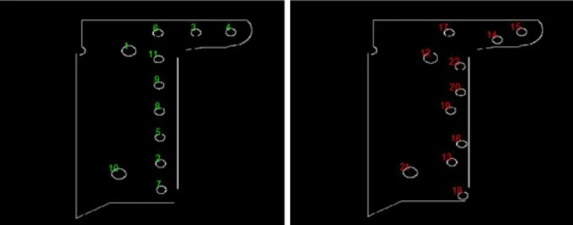
b b)

that will be further matched. Prasad algorithm25 performs good in our image for ellipses detection as soon as the image is correctly segmented. This is also the case for ELSD algorithm26that we will use. The advantage of using ELSD algorithm is that as a result we can obtain both ellipses and line segments using one single algorithm. If the input image is not correctly segmented before primitive extraction by ELSD, as a result we can obtain primitives that are not interesting for the matching (very short segments and concentric circles). In this case a aftermath filtering stage is necessary. One way to deal with this problem should be segment the image first in order to give to the algorithm an image in which the background is uniform with the foreground representing the object containing the features to be extracted. This could be achieved using a segmentation algorithm like region growing, combined with some processing strategies based on mathematical morphology. However, in this paper we are using synthetic images (CAD-derived images) and the real image is a CAD-derived image modified to introduce some flaws. In that sense, feature extraction is made easier as the primitives are known from CAD model specifications. Nonetheless, this segmentation stage will be included in the method when we will integrate acquired images shown in figure 2. Figure 3 shows one example of primitives extracted in CAD-derived image and primitives obtained by modifying the initial primitives from CAD-derived image (these primitives simulate the real primitives). This two set of primitives are the input of our matching method described in the next subsections. As stated previously, we consider two type of primitives, ellipses and line segments. Each type

Figure 3: Set of primitives (line segments and ellipses) from theoretical images (left) primitives obtained by modifying the initial primitives from CAD-derived image. Ellipses are labelled to make their identification

easier in matching stage

of primitive can be described by a set of attributes. One ellipse is represented by five parameters. Its centre coordinates, the orientation angle and the half-length of the two axis. Lines are described by their endpoints.

3.3 Feature matching using a match function

Line segments matching has been a widely studied topic over this last forty years as they can be used in several applications such as 3D reconstruction,29 object retrieval, etc. This is also the case for primitives like ellipses.30 In this subsection we explain our primitive matching method. Figure 3 shows an illustration of such primitives. 3.3.1 Preliminaries

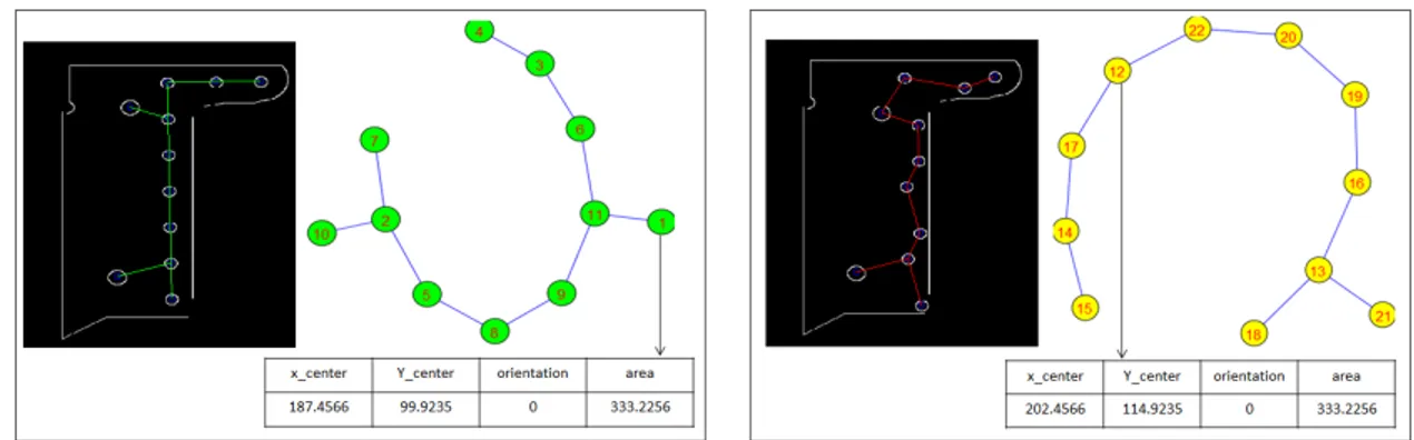
Given two sets of primitives T and R, with T representing primitives in the theoretical image and R representing primitives in the real image, we will show how a match score s(T,R) denoting the similarity between these two sets of primitives can be computed. For ellipses, from the initial five parameters, we create an attribute vector with four variables. The centre coordinates, the orientation angle and the ellipse area (computed using the the half-length of the two axis). For lines, from the endpoints we compute the attribute vector composed of four variables also, the midpoint coordinate of the line, its length and its orientation angle. For each primitive set, we construct a graph (basic concepts of graph theory are presented in the next subsection). The graph representing theoretical primitives is composed of N nodes (for N theoretical primitives) and the one for the real data set contains K nodes (representing the K primitives in the real image). Each graph node is associated with the attribute vector describing the represented primitive. Each graph contains also a set of edges linking two nodes. Two primitives are linked by relative neighbourhood relationship.31 _{However, any other proximity relationship} could be convenient as we are not exploiting the edges relationship, all the relevant information (attributed vector) is assigned to the nodes. The choice of using an attribute graph was made because graph is an effective

Center enter orientation area

187.!566 99.9235 333.2256

way of representing objects,32 standardized and easy to handle (we can assign as many attributes as we wish to nodes and edges). Figure 4 shows two graphs corresponding to the two sets of ellipses presented in fig.3.

Figure 4: Attributed graphs for the two sets of ellipses shown in Fig.3 with an attribute vector associated to one node of each graph as an example.

3.3.2 Basic graph theory concepts

Given a graph G = (V, E) the set NG(v) = u ∈ V (G)|uv ∈ E denotes the neighbourhood of a vertex v. The degree of a vertex v is |NG(v)| and is denoted by dG(v). If dG(v) = 0 then v is called an isolated vertex. The in-degree of a vertex v is the number of edges having the arrow pointing toward v. The out-degree of a vertex v is the number of edges having the arrow going out from v. A graph G = (V, E) is said to be bipartite if V (G) can be partitioned into two disjoint sets T and R such that every edge e ∈ E joins a vertex in T to another vertex in in R. A partition (T, R) of V is called a bipartition. A bipartite graph with bipartition (T, R) of V is denoted by G = (T, R, E). Most of these definitions can be found in33_{and in Python igraph library documentation. Others} standard concepts in graph matching include graph or subgraph isomorphism and maximal common subgraph.34 In graph matching as often as possible exact graph matching is carried out through isomorphism and maximal common subgraph. Other times inexact graph matching is needed.13 _{As said in}21, 34_{in real world applications it} is not always possible to use concepts such as graph isomorphism or maximal common subgraph because of the imperfection of the real word data. In such cases an error-tolerant graph matching approach or a method that computes a measure of similarity between two given graphs is suitable, which is the case in the work described in this paper.

3.3.3 Match function

The match score is computed in the following manner. We divide the attribute variables in two classes (t = 1, 2). Attribute variables such as area or length belong to the first group as they can be computed using their ratio. Variables like centre coordinate or orientation are computed in an other way as their ratio is not meaningful. They are computed using the absolute difference, and their calculus may incorporate the maximal accepted disparity between the theoretical and the acquired primitives. They are in group 2. Our match function is inspired by35 _{(proposed for line matching) and adapted to be able to deal with ellipses also.}

Sti =        min(Ti, Ri) max(Ti, Ri) , if t=1 (1) δi− abs(Ti− Ri) δi , if t=2 (2) s(Tk, Rl) = M F (Tk, Rl) = X StiWi (3)

Where t is the primitive class (1 or 2). Ti is a primitive in the theoretical image. Ri is a primitive in the real image. And i denotes the i-th attribute for the considered primitive. δistands for the maximal accepted disparity

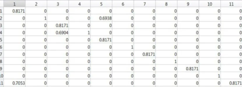
1 2 3 4 5 6 8 9 10 11 1 0.8171 0 0 0 0 0 0 0 0 0 0 2 0 1 0 0 0.6938 0 0 0 0 0 0 3 0 0 0.8171 0 0 0 0 0 0 0 0 4 0 0 0.6904 1 0 0 0 0 0 0 0 5 0 0 0 0 0.8171 0 0 0 0 0 0 6 0 0 0 0 0 1 0 0 0 0 0 7 0 0 0 0 0 0 0.8171 0 0 0 0 8 0 0 0 0 0 0 0 1 0 0 0 9 0 0 0 0 0 0 0 0 0.8171 0 0 10 0 0 0 0 0 0 0 0 0 1 0 11 0.7053 0 0 0 0 0 0 0 0 0 0.8171

for the i-th attribute in class t = 2 and Sti is the match score between one T primitive with one R primitive for

the i-th attribute. In equation (3), k and l stand for l-th theoretical primitive and k-th real primitive respectively. While Wirepresents the weight for the i-th attribute and s(Tk, Rl) denotes the match score between Tk with Rl. The match function is conditioned to be in range of [0, 1] when t = 1. In35_{the similarity score for variables such} as orientation or centre coordinate can be < 0. In our method only candidates having scores in the range [0, 1] for both t = 1 and t = 2 are considered for matching if they satisfy the threshold condition. As some attributes may be more relevant than others13 _{a priority weighting function may be suitable. In our case we follow the} weighting technique proposed by.35 _{The matching algorithm is accomplished by exploring all the nodes in the} theoretical graph and by searching to the most similar nodes in the graph representing the primitives from real image. The similarity criterion used during the search process is the match function described previously. During this process a matching matrix is computed. The matching matrix links a primitive in the set T with a primitive in the R set, cf. figure 5. This matching matrix is very important as it is used later to construct the bipartite graph.

Figure 5: Matching matrix corresponding to ellipses shown in Fig. 3. For this result, the matching threshold is fixed to 0.5. The maximal disparity accepted for attributes corresponding to the centre coordinates is 40 pixels

and 10◦ in orientation.

3.4 Search of mutual best match in a bipartite graph

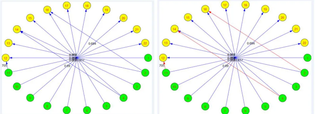
Bipartite graph matching has been widely studied and have applications in various field of science as in data mining,36 _mathematics,33 _{computer vision or image analysis.}20, 21, 37 _{And by its definition it is obvious that it is} particularly suitable for a two-class matching. In our method it is used as follows. First we count the number M of occurrences of a score in the matching matrix meeting a predefined threshold. A bipartite directional graph containing M nodes is then created. This graph holds in it two types of nodes (T , R), representing theoretical and real primitives respectively. A T type node in the bipartite graph is linked (edge from T type node) with a R type node when their similarity score satisfies the threshold condition. The edge linking these two nodes is weighted with their similarity score. Depending on the threshold value, which has to be low in order not to reject potential match candidates, one T type node may be connected to more than one R type node and reversely. In that sense, an optimization process is required in order to filter out edges having low score and keep uniquely the mutual best matches. The mutual best match search algorithm in the bipartite graph is divided in two stages. In the first stage best matches are found for edges linking a R type node with a T type node as follows : Let k be a node R type, if the in-degree of k is 1, add the edge linking k and one T type node to the best match edge list. Otherwise, if the in-degree of k is greater than 1, then search the connected edge to k holding the maximal weight. Add this edge to the best match edge list. Add the other edges to the pruning list. As the edges in the bipartite graph are oriented, this step can be considered as a target-to-source best search. In the second stage the best matches in source-to-target sense are found, using the out-degree of the nodes. The mutual best match are kept and all non mutual best match edges are eliminated from the graph. The mutual best match search is carried out by prudence. If it is obvious that a source-to-target best match search is not satisfactory because it can lead to two source nodes (T type nodes) having the same target (R type node) which violates the uniqueness constraint in the matching. On the other hand, the target-to-source best match search (finding the best edge coming to a R type node) can be sufficient to find the true best matches as it is very unlikely to a non best match edge coming to a R type node to have a better weight than a best match edge coming to another R type node. Figure 6 shows the bipartite graph before and after the mutual best match search.

o

m

®

®

.:-,a.

:

"

Figure 6: Mutual best match illustration. Left: bipartite graph weighted with the scores from the matching matrix, before mutual best match search. Right: bipartite graph with mutual best match coloured in blue and

non best matches in red.

3.5 Match reinforcement

After the matching stage, we carry out a reinforcement match operation, based on the topology of the matched primitives. Let T0 and R0 be the set of matched primitives, that means that one element in the set T0 matches only and only one element in the set R0 after best match procedure. So T0 and R0 are subsets of T and R sets and they have the same dimensions. The match reinforcement is made as follows. Two neighbourhood graphs are constructed using the Gabriel proximity graph (Correa paper31 _{provides a good literature on proximity} graphs). One for the T0 set (CAD-derived primitives) and the other one for the R0set. Remember our approach is guided by the information from the CAD model. That means that the primitives from the CAD-derived image stand as the reference in the matching process. The assumption made here is that if the matches are congruent, the two graphs of best match primitives will have the same topology. A node in T0 set will have the same number of neighbours that his corresponding node from R0 has. In addition their respective neighbours will be approximatively at the same distance and the same orientation. A threshold for the distance has to be defined and the maximal accepted disparity in orientation needs to be defined also. If this threshold and the maximal accepted orientation are satisfied for elements in T0 and R0 then our confidence in the match process is strengthened. The match pair that does not obey this criterion should be removed or reviewed. This reinforcement match function could not be introduced as is during the match operation because the set T and R are not necessary the same dimension, R can contain more primitives than T (artefacts) or less primitives than T (missing element or failure during the primitive extraction stage)

4. RESULT,

DECISION, DISCUSSION AND FUTURE WORK

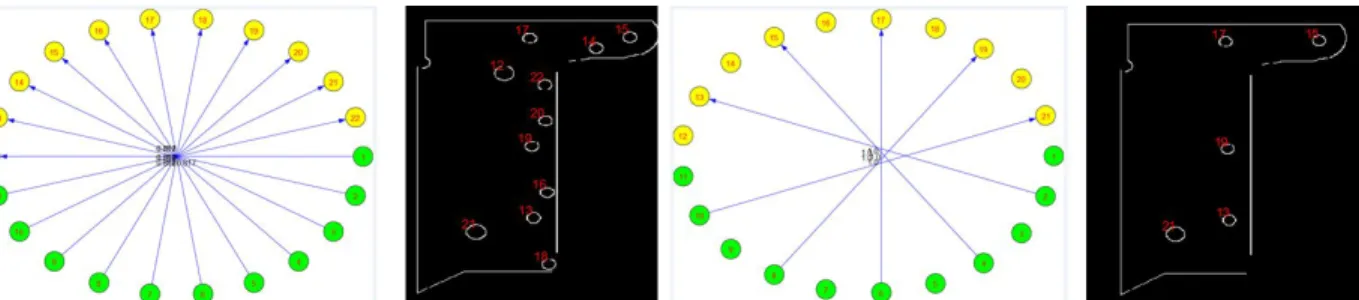
The present method was tested with synthetic data and has proved to work well. It is capable of finding correct matches for ellipses and for line segments. Test cases include missing elements, displaced elements, size changes, and combination of these cases. In all these cases the method performs well. In the end of the matching procedure, for each primitive type (ellipse or line segment) the final score is the number of matches returned by the method out of the number of primitives in the CAD-derived image. Thus, these scores need to be combined in order to make the decision about element conformity. If all the primitives are supposed to be of equal importance, then a mean can be computed and compared with a threshold. As the initial matches are found using a threshold (which is set to a low value eg. 0.5 in order not to discard correct matches) matches with low values of similarity may be found. Therefore, it is suited to choose a convenient value of threshold in order to maximize the similarity between the tested element and the theoretical element. Figure 7 illustrates this problem. A trade-off has then to be attained. When the threshold value is set to 0.5 all the matches are found. But when the threshold is higher (0.85) only 5 primitives out of 11 find a match. An other relevant point is attribute weights. As several attributes are used in the method, it may be suited to give rather more importance to some of them than to others.13 We use the weighting function defined by.35 Even if we gave equal weights to the attributes during the testing phase it is worthy to remember that their weights are parametrizable. As said in sec. 3.2 real images shown in figure 2 will be introduced later, in order to have a fully automated inspection method based on 2D

t

'b/

'b

ò

Figure 7: Two test cases. From the left to the right : bipartite graph showing the best matches for a threshold set to 0.5; image showing the tested primitives having a match; bipartite graph showing the best matches for a

threshold set to 0.85; image showing the tested primitives having a match;

based matching using CAD data. Objectives of future works include also how CAD model can be used for direct comparison with a 2D image (without generating images from the model).

REFERENCES

[1] Modayur, B., Shapiro, L., and Haralick, R., “Visual inspection of machined parts,” Computer Vision and Pattern Recognition (June 1992).

[2] Newman, T. and Jain, A. K., “A survey of automated visual inspection,” Computer Vision and Image Understanding 61 (1995).

[3] Malamas, E., Petrakis, E., Zervakis, M., Petit, L., and Legat, J.-D., “A survey on industrial vision systems , applications and tools,” Image and Vision Computing 21, 171–188 (February 2003).

[4] Golnabi, H. and Asadpour, A., “Design and application of industrial machine vision systems,” Robotics and Computer-Integrated Manufacturing 23, 630–637 (December 2007).

[5] Bukovec, M., Spiclin, Z., and F.Pernus, “Automated visual inspection of imprinted pharmaceutical tablets,” Meas. Sci.Tech. 18, 29212930 (2007).

[6] Mozina, M., Tomazevic, D., Pernus, F., and Likar, B., “Automated visual inspection of imprint quality of pharmaceutical tablets,” Machine Vision and Applications 24, 6373 (2013).

[7] Far, A. B., Analyse multi-images Application `a l’extraction contrˆo´ee d’indices images et `a la d´etermination de descriptions sc´eniques, PhD thesis, Louis Pasteur University, France (2005).

[8] Bourgeois, S., Alignement d’Objets M´ecaniques Complexes par Vision Monoculaire, PhD thesis, Clermont Ferrand University, France (2006).

[9] Karabagli, B., V´erification automatique des montages d’usinage par vision : Application `a la s´ecurisation de l’usinage, PhD thesis, Toulouse University, France (2013).

[10] Melnik, S., Garcia-Molina, H., and Rahm, E., “Similarity flooding : A versatile graph matching algorithm and its applications to schema matching,” Proceedings 18th International Conference on Data Engineering , 117 – 128 (February 2002).

[11] Bator, M. and Nieniewski, M., “Detection of cancerous masses in mammograms by template matching: Optimization of template brightness distribution by means of evolutionary algorithm,” J Digit Imaging 25, 162–172 (2012).

[12] Lowe, D. G., “Distinctive image features from scale-invariant keypoints,” IJCV 2 (2004).

[13] Jr., R. M. C., Bengoetxea, E., Bloch, I., and Larra˜naga, P., “Inexact graph matching for model-based recognition: Evaluation and comparison of optimization algorithms,” Elsevier, Pattern Recognition 38, 2099–2113 (2005).

[14] Bay, H., , Tuytelaars, T., and Gool, L. V., “SURF: Speeded Up Robust Features,” ECCV 3951, 404–417 (2006).

[15] Stefano, L. D., Mattoccia, S., and Tomabari, F., “ZNCC-based template matching using Bounded Partial Correlation,” Pattern Recognition Letters 26, 2129–2134 (2005).

[16] Briechle, K. and Hanebeck, U. D., “Template matching using fast normalized cross correlation,” Optical Pattern Recognition XII (2001).

[17] Bai, X. and Latecki, L. J., “Path similarity skeleton graph matching,” Pattern Analysis and Machine Intelligence 30, 1282 – 1292 (2008).

[18] Xu, Y., Wang, B., Liu, W., and Bai, X., “Skeleton graph matching based on critical points using path similarity,” Computer Vision ACCV 2009, Lecture Notes in Computer Science 5996, 456–465 (2010). [19] Hilaga, M., Shinagawa, Y., Taku, and Kunii, T. L., “Topology matching for fully automatic similarity

esti-mation of 3d shapes,” ACM SIGGRAPH. Proceedings of the 28th annual conference on Computer graphics and interactive techniques , 203–212 (2001).

[20] Fishkel, F., Fischer, A., and Ar, S., “Verification of engineering models based on bipartite graph matching for inspection applications,” Springer-Verlag Berlin Heidelberg. LNCS 4077 , 485–499 (2006).

[21] Shokoufandeh, A. and Dickinson, S., “Applications of bipartite matching to problems in object recognition,” ACM, Proceedings of ICCV on Graph Algorithm and Computer Vision (1999).

[22] Duda, R. O. and Hart, P. E., “Use of the Hough Transformation to detect lines and curves in pictures,” Coomunications of ACM 15, 11–15 (1972).

[23] McLaughlin, R. A., “Randomized Hough Transform: Improved ellipse detection with comparison,” Elsevier, Pattern Recognition Letters 19, 299305 (1998).

[24] von Gioi, R. G., Jakubowicz, J., Morel, J.-M., and Randall, G., “Lsd: a line segment detector,” Image Processing On Line : http: // dx. doi. org/ 10. 5201/ ipol. 2012. gjmr-lsd (2012).

[25] Prasad, D. K., Leung, M. K., and Quek, C., “Ellifit: An unconstrained, non-iterative, least squares based geometric ellipse fitting method,” Pattern Recognition 46, 14491465 (2013).

[26] Patraucean, V., Gurdjos, P., and von Gioi, R. G., “A parameterless line segment and elliptical arc detector with enhanced ellipse fitting,” Computer Vision ECCV 2012, 2th European Conference on Computer Vision, Proceedings, Part II 46, 572–585 (2012).

[27] Wang, G., Ren, G., Wu, Z., Zhao, Y., and Jiang, L., “A fast and robust ellipse-detection method based on sorted merging,” Hindawi Publishing Corporation, The Scientific World Journal (2014).

[28] Nguyen, T. M., Ahuja, S., and Wu, Q., “A real-time ellipse detection based on edge grouping,” IEEE International Conference on Systems, Man and Cybernetics , 3280 – 3286 (October, 2009).

[29] Bay, H., Ferrari, V., and Gool, L. V., “Wide-baseline stereo matching with line segments,” Proceedings of Computer Vision and Pattern Recognition 1, 329–336 (2005).

[30] Hutter, M. and Brewer, N., “Matching 2-d ellipses to 3-d circles with application to vehicle pose identifica-tion,” Proceedings of International Conference Image and Vision Computing , 153 – 158 (2009).

[31] Correa, C. D. and Lindstrom, P., “Locally-scaled spectral clustering using empty region graphs,” ACM, Proceedings of the 18th ACM SIGKDD international conference on Knowledge discovery and data mining , 1330–1338 (2012).

[32] Bengoetxea, E., Inexact Graph Matching Using Estimation of Distribution Algorithms, PhD thesis, Ecole Nationale Sup´erieure des T´el´ecommunications, Paris, France (Dec 2002).

[33] Panda, B. and Pradhan, D., “Minimum paired-dominating set in chordal bipartite graphs and perfect elimination bipartite graphs,” Journal of Combinatorial Optimization 26, 770 – 785 (2013).

[34] Bunke, H., “Graph matching: Theoretical foundations, algorithms, and applications,” In International Conference on Vision Interface (2000).

[35] McIntosh, J. H. and Mutch, K. M., “Matching straight lines,” Computer Vision, Graphics and Image Processing 43, 386–408 (1988).

[36] Zha, H., He, X., Ding, C., Simon, H., and Gu, M., “Bipartite graph partitioning and data clustering,” ACM, Proceedings of the tenth international conference on Information and knowledge management , 25–32 (2001).

[37] Wang, C. and Ma, K.-K., “Bipartite graph-based mismatch removal for wide-baseline image matching,” Journal of Visual Communication and Image Representation 25, 1416–1424 (2014).