A fast and versatile method for spectral emissivity measurement at high temperatures

(1)

HAL Id: hal-02375277

https://hal-mines-albi.archives-ouvertes.fr/hal-02375277

Submitted on 27 Nov 2019

HAL is a multi-disciplinary open access archive for the deposit and dissemination of sci-entific research documents, whether they are pub-lished or not. The documents may come from teaching and research institutions in France or abroad, or from public or private research centers.

L’archive ouverte pluridisciplinaire HAL, est destinée au dépôt et à la diffusion de documents scientifiques de niveau recherche, publiés ou non, émanant des établissements d’enseignement et de recherche français ou étrangers, des laboratoires publics ou privés.

A fast and versatile method for spectral emissivity

measurement at high temperatures

Abdelmagid El Bakali, Rémi Gilblas, Thomas Pottier, Yannick Le Maoult

To cite this version:

Abdelmagid El Bakali, Rémi Gilblas, Thomas Pottier, Yannick Le Maoult. A fast and versatile method for spectral emissivity measurement at high temperatures. Review of Scientific Instruments, American Institute of Physics, 2019, 90 (11), pp.115116-1 - 115116-19. �10.1063/1.5116425�. �hal-02375277�

(2)

1

A fast and versatile method for spectral

emissivity

measurement

at

high

temperatures

Abdelmagid El Bakali1*_{, Rémi Gilblas}1_{, Thomas Pottier}1_{, Yannick Le Maoult}1

(1) Institut Clément Ader (ICA) ; Université de Toulouse ; CNRS, IMT Mines Albi, INSA, ISAE-SUPAERO, UPS ; Campus Jarlard, F-81013 Albi, France

1* corresponding author: aelbakal@mines-albi.fr

Keywords: Spectral emissivity, Total emissivity, Platinum, IR spectrometry, IR thermography, High temperature, Direct radiometric methods, IR heating, Elliptical furnace

Abstract: In this paper, the development of a new device for high temperature emissivity measurement is described. This device aims at measuring both spectral and total emissivity for a thermal range of 600 to 1000°C. The device main targeted properties were both versatility and simplicity. To do so, a rigorous selection was made for each component: heating system, heat source, sample holder, measuring devices. Sample dimensions and the corresponding sample holder were optimized through a ray tracing model computation. Selection of sensors to compute a total emissivity was also especially discussed. A NIR spectrometer, and two MIR cameras covering [3-5] and [7.5-13]µm equipped with optical filters were chosen for spectral measurements. The major impediment was the separation between sample signal and various spurious signals emitted by environment. A specific measurement methodology was then made for each bandwidth to resolve this issue. A reference material was chosen for the device validation: Platinum. Spectral emissivity measurements were then compared to values from a commercial spectrometer. A good agreement was found for NIR and the first MIR band measurements and a higher error was seen in MIR second band which is explained by a less favorable signal to noise ratio. Integrated emissivity is then calculated and compared to values found in the literature. A good agreement between those values is found and similar trends with temperature are observed. The device is then validated for spectral and total emissivity measurement. Device versatility and simplicity allows an easy adaptation to a large area of applications.

This is the aut

hor’s peer reviewed, accepted manuscript. Howe

ver, the online

version of record will be different

from this

version

once it has bee

n copyedited an d typeset. PLEASE CIT E THIS ARTI C LE AS DOI: 10.1063/1.5116425

(3)

2

Introduction

Development of numerical simulation and radiative thermometry in recent years has led to an increasing need for emissivity experimental assessment. Emissivity is a complex property that can be declined in directional spectral emissivity, directional total emissivity, spectral hemispherical emissivity or total hemispherical emissivity [1]. In practice, total hemispherical and spectral directional emissivities are the most needed properties. Total hemispherical emissivity is generally used as a boundary condition for classical heat transfer computation or in surface to surface radiative models. It is therefore the most common and spread out value of emissivity. It is usually determined with devices like thermopile or bolometers [2]… On the other hand, spectral directional emissivity is useful for infrared temperature measurements with devices (IR pyrometer, IR camera…) operating within a specific bandwidth [3]. Indeed, spectral emissivity may exhibit significant variations with the wavelength [4] and having the corresponding spectral emissivity is compulsory in assessing the measurement metric.

Emissivity depends on numerous parameters such as material roughness, chemical composition, manufacturing process, surface oxidation, temperature ([5], [6]). Emissivity values found in literature usually lack such information about the sample used for the measurement. This uncertainty on emissivity can be problematic for applications where accuracy is required (thermoforming, hot stamping…). Commercial devices can generally be used up to 400°C for spectral emissivity which is particularly suitable for thermoplastic and thermoplastic composite materials. However, it is insufficient for high temperature metallic materials applications such as hot forming [7], superplastic forming [8], hot stamping [9]… Another issue for metallic materials is the impact of oxidation at high temperature which strongly modifies emissivity value [6] during the process. In order to have realistic heat transfer calculation or IR measurements for those processes, corresponding materials emissivity have to be measured in the same experimental conditions (temperature, atmosphere, heating rate…). Accordingly, the present paper details the development of a novel apparatus which enables emissivity measurement at high temperatures. Thermal range was guided by usual metal temperature forming range of 600 to 1100°C in aforementioned processes. Bandwidth was selected to match with corresponding bandwidths of most IR detectors[10]: NIR band I (BI): [0.9-2] µm, MIR Band II (BII): [2.5-5] µm, and MIR Band III (BIII): [7.5-13] µm. Furthermore, an integrated emissivity close to total emissivity can be calculated from these bandwidths. Indeed, for a black body heated at 600°C, Wien’s displacement law enables to calculate the maximum emission wavelength:

λmax=2898/T(K) (1)

Then, 96% of the radiation is emitted from 0.5λmax to 5λmax. For the lowest temperature of our

requirements (600°C), the radiation is then emitted between 1.65 and 16.5 µm. For the highest temperature (1100°C), the spectral range is [1.06-10.6] µm. From those calculations, the requirements of the measurement can be built.

Temperature range Bandwidth atmosphere

[600;1100]°C [1.1;16.5]µm Air, vacuum, argon

Table 1 : Device requirements

The main targeted properties for this device are both versatility and simplicity. In one hand, versatility opens a wide range of applications, like solar, spatial, forming applications, temperature measurements or numerical simulation. Therefore, heating and detection systems have to be flexible

This is the aut

ver, the online

from this

version

once it has bee

(4)

3

enough to perform both spectral ant total emissivity measurements while being able to easily modify heating and/or atmospheric conditions. On the other hand, simplicity is wanted to have a standalone device with a good cost-efficiency, which can be successfully implemented in non-specialist operators.

This paper is organized as follows: the first part exposes the state of the art of emissivity measurement methods. A comparison between those methods is then proposed in order to select the most suitable method. The second part describes the device development based on the method selected in the first part. Device elements are optimized to match the temperature requirements presented in Table 1. In the third part, the selection of the different sensors is detailed to comply bandwidth requirements presented in Table 1. Those sensors are then calibrated with a blackbody for the emissivity measurement. In the fourth part, an emissivity measurement is performed on a reference material (pure Platinum).

1. State of art and choice of the measurement method

In this section, most of the common methods dedicated to emissivity measurement are presented in a non-exhaustive list of devices. A comparison is then made between those methods to select the most suited for hot forming applications.

1.1. Theoretical basis

Thermal radiation is emitted by every object with a temperature higher than absolute zero. This radiation is represented theoretically by the radiance that is expressed by the cross product of surface emissivity material and radiance emitted by a blackbody [11]:

𝐿_𝜆(𝜆, 𝜃, 𝜑, 𝑇) = 𝜀(𝜆, 𝜃, 𝜑, 𝑇) ∗ 𝐿0_{(𝜆, 𝜃, 𝜑, 𝑇)} ₍₂₎

Where 𝐿𝜆 is the monochromatic radiance and 𝜀 is the surface emissivity. Radiance is defined as the

emitted flux per surface and solid angle. Those parameters depend on wavelength, direction and temperature. Emissivity can then be defined as the ratio between the radiance emitted by the sample and the radiance emitted by the blackbody at the same temperature [11].

𝜀(𝜆, 𝜃, 𝜑, 𝑇) =𝐿𝜆(𝜆, 𝜃, 𝜑, 𝑇)

𝐿0_{(𝜆, 𝜃, 𝜑, 𝑇)} (3)

This parameter known as directional spectral emissivity can be integrated in space to obtain a spectral hemispherical emissivity (Eq.4). Recalling that a blackbody emission is, by definition, isotropic, the (Eq.4) can then be simplified as follows (Eq.5).

𝜀(𝜆, 𝑇) =∫ ∫ 𝜀(𝜆, 𝜃, 𝜑, 𝑇) ∗ 𝐿 0_{(𝜆, 𝜃, 𝜑, 𝑇) ∗ 𝑐𝑜𝑠𝜃 ∗ 𝑠𝑖𝑛𝜃 ∗ 𝑑𝜃 ∗ 𝑑𝜑} 2𝜋 0 𝜋 2 ⁄ 0 ∫ ∫2𝜋𝐿0_{(𝜆, 𝜃, 𝜑, 𝑇) ∗ 𝑑𝜃 ∗ 𝑐𝑜𝑠𝜃 ∗ 𝑠𝑖𝑛𝜃 ∗ 𝑑𝜑} 0 𝜋 2 ⁄ 0 (4) 𝜀(𝜆, 𝑇) =∫ ∫ 𝜀(𝜆, 𝜃, 𝜑, 𝑇) ∗ 𝐿 0_{(𝜆, 𝑇) ∗ 𝑐𝑜𝑠𝜃 ∗ 𝑠𝑖𝑛𝜃 ∗ 𝑑𝜃 ∗ 𝑑𝜑} 2𝜋 0 𝜋 2 ⁄ 0 𝜋 ∗ 𝐿0_{(𝜆, 𝑇)} (5)

Directional spectral emissivity can also be integrated over wavelength to obtain a directional total emissivity (Eq.6). This latter relation (Eq.6) can then be simplified by integrating blackbody radiance over all wavelengths (Eq.7) [10].

This is the aut

ver, the online

from this

version

once it has bee

(5)

4 𝜀(𝜃, 𝜑, 𝑇) =∫ 𝜀(𝜆, 𝜃, 𝜑, 𝑇) ∗ 𝐿 0_{(𝜆, 𝑇) ∗ 𝑑𝜆} ∞ 0 ∫ 𝐿∞ 0_{(𝜆, 𝑇) ∗ 𝑑𝜆} 0 (6) 𝜀(𝜃, 𝜑, 𝑇) =∫ 𝜀(𝜆, 𝜃, 𝜑, 𝑇) ∗ 𝐿 0_{(𝜆, 𝑇) ∗ 𝑑𝜆} ∞ 0 𝜎𝑇4 𝜋 ⁄ (7)

Finally the total hemispherical emissivity can be obtained by integrating over both wavelength and direction (Eq.8). This equation can be simplified by using (Eq.4) aiming to only have integration over wavelength (Eq.9). 𝜀(𝑇) =∫ ∫ ∫ 𝜀(𝜆, 𝜃, 𝜑, 𝑇) ∗ 𝐿 0_{(𝜆, 𝑇) ∗ 𝑐𝑜𝑠𝜃 ∗ 𝑠𝑖𝑛𝜃 ∗ 𝑑𝜃 ∗ 𝑑𝜑 ∗ 𝑑𝜆} ∞ 0 2𝜋 0 𝜋 2 ⁄ 0 ∫ ∫ ∫ 𝐿∞ 0_{(𝜆, 𝑇) ∗ 𝑐𝑜𝑠𝜃 ∗ 𝑠𝑖𝑛𝜃 ∗ 𝑑𝜃 ∗ 𝑑𝜑} 0 2𝜋 0 𝜋 2 ⁄ 0 ∗ 𝑑𝜆 (8) 𝜀(𝑇) =∫ 𝜀(𝜆, 𝑇) ∗ 𝐿 0_{(𝜆, 𝑇) ∗ 𝑑𝜆} ∞ 0 𝜎𝑇4 𝜋 ⁄ (9)

As explained above, the total hemispherical emissivity 𝜀(𝑇) and the spectral directional emissivity 𝜀(𝜆, 𝑇, 𝜃, 𝜑) are the most sought values especially for high temperatures (numerical simulation and IR measurement). For both quantities, a high accuracy on the sample temperature is needed, even more for metallic materials whose emissivity is often varying with temperature. Several methods exist to determine these emissivities and will be described in the following. They can primarily be sorted in two main categories: i) the so-called direct methods, based on the emissivity definition which is directly calculated from the ratio of the radiance of a sample and the blackbody’s one at the same temperature and ii) the indirect methods, assessing emissivity from the spectral reflectance of an opaque material by an application of Kirchhoff’s law(Eq.10) which, in this case, reads:

𝜀(𝜆, 𝑇, 𝜃, 𝜑) = 1 − 𝜌(𝜆, 𝑇, Ω)

With Ω = ∬ 𝑠𝑖𝑛𝜃. 𝑑𝜃. 𝑑𝜑_𝑠 (10)

Both direct and indirect methods provide spectral directional emissivity. It is then possible to determine a total hemispherical emissivity from spectral and spatial integration (if the bandwidth is wide enough for a given temperature).

1.2. Emissivity measurement methods

1.2.1. Indirect methods

In such approaches, the emissivity is generally assessed from reflectivity (see Eq. 10).

For spectral directional emissivity, surface reflectance 𝜌(𝜆, 𝑇, Ω) can be measured by various techniques such as FT-IR spectrometry equipped with an integrating sphere [12]. A high reflecting coating is applied on the internal surface of the sphere. An incident beam is directed on the sample and the following reflected flux by the sample in every direction is reflected by the sphere until it reaches the detector.

Alternatively, collecting the reflected flux all over the hemisphere can be performed by a set of mirrors (as high as 20), as in the spectrophotometry technique developed by Makino and Wakabayashi [13] [14]. This system can provide a measurement of directional spectral reflection for a bandwidth between 0.3 and 11µm. This technique allows a fast measurement over a wide range of wavelength but is limited by the directional nature of the measure and also by the complexity of the optical paths required to redirect the reflected flux (mirrors and diffraction gratings). Reflectance can

This is the aut

ver, the online

from this

version

once it has bee

(6)

5

also be measured from mirror-based techniques. In such configuration, the sample and the detector are both placed inside a hemispherical mirror. The sample then reflects an incoming light beam that passes through a hole in the mirror. The detector thus collects the reflected heat flux from every direction and provides a measurement of the directional hemispherical reflectivity. In such approach, only one incidence angle can be investigated at a time. Later works have proven possible the evolution of this technique for varying incidence angles [15]. In this latter paper, Hameury et al. have used serval holes in the mirror to reach 5 different angles of incidence ranging from 12° to 60°. Nevertheless, in such configuration, optical paths become complex and requires many optical components and the system ultimately loses the inherent simplicity of mirror-based devices.

An alternative method developed by Fu and al. is based on the illumination of a sample by 6 150mm long quartz lamps. Located at the periphery of a hemisphere, these conditions lead to the measurement of reflectance, directly linked with emissivity as denoted by equation 10. Performing the measurement at 10 wavelengths with a spectrometer, the method enables to determine on-line the temperature, the emissivity and the lamp radiance for each wavelength. This method is inherently few sensitive to temperature knowledge but is valid only for diffuse surfaces.

Another active indirect method is thermoreflectometry[16][17]. The aim of this method is to measure an object true temperature from thermography with a direct correction of the emissivity at two wavelengths. This latter correction being achieved from the reflection of two laser beams illuminating the sample at 1.3 and 1.55 µm. The advantage of this technique is the time-continuous nature of the measurement of emissivity at high temperatures. The constraints are the need of flat and opaque sample and the fact that emissivity measurement is limited to two wavelengths.

Total directional emissivity can be obtained by numerical integration of directional hemispherical

reflectivity presented before, but also by operating the reflectivity measurement with a very wide band source (heated carbide ring) and detector (pyroelectric, bolometric and/or thermopile[19]). The challenge is here to set the spectral bandwidth to ensure that all the reflected flux is detected for every wavelength.

The measurement of spectral hemispherical emissivity can be performed using a BRDF (Bidirectional Reflectivity Distribution Function) apparatus [20] (similar to a goniometer module), scanning every incident and reflection angle of the hemisphere, often provided for a single wavelength defined by the laser source wavelength.

The calculation of total hemispherical emissivity is possible using an integrating sphere and a very wide band source and detector. Choosing the BRDF option [21] is still possible, but with a source and detector which wavelength is adjustable.

To sum up, indirect methods are rather simple to set up for the measurement of spectral directional emissivity but turn out to be optically complicated for hemispherical reflectivity measurement.

1.2.2. Direct methods

Direct radiometric method techniques are well suited for high temperature since they usually involve less optics [22]. They are based on the direct evaluation of the definition of the emissivity provided in equation 3. The main difficulty is to ensure that the sample and the blackbody exhibit the exact same

This is the aut

ver, the online

from this

version

once it has bee

(7)

6

temperature. Another difficulty is to maintain a homogeneous temperature across the sample measurement field.

For the spectral directional emissivity, the radiation is detected in a unique direction or a small solid angle by sensors and the sample temperature is controlled which thermocouples [23], pyrometer [24], IR camera [25], pyroreflectometer [26] or the use of Christiansen point [27]. Literature also provides several examples of heating techniques: thermostatic fluid [28], laser [24], electrical [23] or radiative heat sources [26]. Finally, the reference body can be either a laboratory blackbody [29] or a known high emissive sample [30].

An example of direct method is the so-called furnace drop technique proposed by Dozhdilkov et al. [31]. This technique consists in inserting the sample inside a commercial cavity blackbody until the sample temperature stabilizes. Then, the blackbody is dropped (meaning that the sample is rapidly extracted from the cavity) and the sample radiance is measured. Knowing the blackbody radiance at the same temperature, emissivity can then be deduced following Eq.3.

As mentioned in the title of Dozhdilkov et al. paper, this technique uses transient thermal states and is therefore not suited for high conducting materials. Another significant drawback is the inability to perform a continuous measure of emissivity and therefore investigate oxidation phenomenon. A more recent development is the work of the LNE laboratory [26]. The sample is placed in a vacuum chamber and heated up by 7 IR halogen lamps through a quartz hemispherical dome. Signal emitted by the downside face of the sample is directed toward an IRTF spectrometer. Measurements can be performed for a bandwidth between 0.8 and 10µm. The reference blackbody is a SiC cavity whose temperature is controlled by a S thermocouple. A pyroreflectometer[32] is used to measure the sample temperature. Such radiative sources enable versatile heating with steep temperature rises. A maximum operating temperature of 1500°C is reported.

The latest development of direct methods facilities is detailed in a work of the Beijing Institute [33]. The back side of the sample is heated up by a furnace (T <1000°C) while the front side faces a parabolic mirror. The mirror is setup on a rotary stage in order to face alternatively the sample and the cavity of a commercial blackbody. The emitted flux is then directed in an InGaAs detector which only allows an emissivity measurement over the NIR (0.8 to 2.2 µm) bandwidth.

It is worth noticing that the last two techniques do not allow an easy evolution toward measurement under inert gas atmosphere, they are therefore hardly applicable in the field of high temperature metals.

Another device has also been developed recently by CEMHTI [34]. An interesting particularity of this device is that it can be applied to semitransparent materials. A normal spectral emissivity can be measured for a wide bandwidth (0.5 to 500µm) through two spectrometers. Sample is heated by a ceramic plate heater for T<1200K and by a CO2 laser for higher temperatures which allows measurements between 700 and 2500K. Advantages of this device are the wide temperature range, wide bandwidth which allows calculating integrated emissivities and an application for both opaque and semitransparent materials. Sample temperature measurement is done through Christiansen point which is a wavelength where emissivity is equal to 1 for dielectric materials. For metallic samples, a thermocouple or the use of χ point (for pure metals) which is a wavelength where

This is the aut

ver, the online

from this

version

once it has bee

(8)

7

emissivity is invariant versus T can be used to determine sample temperature. Drawbacks are the complexity of the heating system with a set of mirrors to homogenize the sample temperature for the laser configuration. Another drawback is temperature measurement for metallic sample that don’t have Christiansen point and implies the knowledge of the χ point.

Total directional emissivity can be obtained by numerical integration of spectral directional

emissivity. Another issue would be to use a very wide bandwidth detector comparing the integrated flux of the sample with the one emitted by a blackbody at the same temperature.

For the measurement of spectral hemispherical emissivity, an integrating sphere is required to detect the emitted flux in the entire hemisphere. Another set-up would be a goniometer apparatus enabling the measurement of the emitted flux for different directions[35]. A spatial integration would then be necessary to retrieve the hemispherical quantity.

Finally, the total hemispherical emissivity can be obtained with an integrating sphere operating over a very wide spectral range or a goniometer module measurement the radiation for every directions and every wavelengths [36]. However, the most famous and certified method for evaluating this quantity is still the well-known calorimetric method [37],[38]. These methods are interesting because the total hemispherical emissivity can be directly measured. For this method the sample is heated to a fixed temperature (Ts) with an electrical resistance. The sample is then inserted into a black vacuum chamber with the internal wall temperature (Tw) maintained by liquid nitrogen or liquid helium. The power applied (P) to the sample is adjusted to maintain a constant temperature (Ts). The vacuum chamber enables to nullify the convective heat exchange. Emissivity can then be calculated by the following formula (eq. 11):

𝜀 = 𝑃

𝑆 ∗ 𝜎 ∗ (𝑇_𝑠4− 𝑇_𝑤4₎ (11)

Where σ is the Stefan-Boltzmann constant and S stands for the sample surface area. The main advantages of the calorimetric method are the simplicity of the measurement principle and the fact that the total emissivity is easily deduced for several temperatures. Moreover, transient measurements can also be performed. The main drawback being that no spectral information can be obtained from such experiment. In addition, some experimental issues have led to reconsider such approaches. Indeed it is often difficult to maintain a homogeneous temperature over the sample, the stabilization time can be significant, and maintaining the environment (especially the walls temperature) can be very challenging.

1.3. Method selection

The choice of the method, based on the requirements of the measurement, is performed by comparison between several criteria like complexity of the system, atmosphere versatility… Some methods like integrating sphere were automatically eliminated due to the complexity of the adaptation to high temperature.

This is the aut

ver, the online

from this

version

once it has bee

(9)

8

Method Calorimetric Indirect Direct

Devices [39] [40] [41] [14] [15] [17] [25] [26] [33] [34]

Spectral emissivity None None None [2;11]µm [0.8;11] _µm 1.3 and _1.55µm [1.28;25]µm [0.8;10]µm [0.2;2.2]µm [0.5;500]µm Total

hemispherical emissivity

OK OK OK None None None None None None None

Material

application Metal Metal Metal

Opaque, metal Opaque, metal Opaque, metal Opaque, metal Opaque, metal Opaque, metal Opaque, semi-transparent Temperature range (°C) [300;1000] [-20;80] [177;677] Up to 827 Ambient [300;1000] [25;777] Up to 1500 [200;1000] [427;2227] Sample temperature measurement S type thermocou ple K type thermoc ouple S type thermocou ple K type thermoco uple None Active thermorefl ectometry K type thermocouple Pyroreflecto metry K type thermocoupl e Christiansen point χ point Heating method Electrical

Thermof oil heater

Electrical Halogen _lamp _sourceLamp

Independe nt of the method Resistive spiral wire Halogen lamp Iron plate

heater Laser heating Heating rate Unknown Unknow_n Unknown 1 K/s None

Independe nt of the method

Unknown Quick Unknown Unknown

Atmosphere Vacuum Vacuum Vacuum Air Air

Independe nt of the method

Vacuum Vacuum Air Argon

Table 2 : Comparison of emissivity measurement methods[39][40][41][14][15][17][25][26][33][34] The aim of the proposed device here is to allow measurement of both spectral and integrated emissivity at high temperatures. Under such conditions, the calorimetric methods can be discarded since they are not suited for spectral applications. Direct methods devices are more adapted for high temperature applications and are usually simpler in their conception comparatively to indirect method devices. The choice is then made for a direct method based device with IR heating system to have high and flexible heating rate, even if devices are usually built-in and weighty. The difficulty then lies in the development of a standalone, fast, user-friendly, versatile and cheap device able to provide both spectral and integrated emissivity measurements. IR lamp is chosen (rather than laser) to simplify the system and to lower its cost. Moreover, IR heating is more suited to metallic materials than laser heating. Indeed, thanks to its wide emission spectrum, IR lamps focus more on the spectral domain where absorption is high (short wavelengths). Moreover, because of its high power spectral density, laser heating induces the risk to burn or modify the sample surface, which is penalizing for

the measurement. In addition, such heating principle is very close to classical industrial heating

systems (in term of chromaticity, heating rates, surface power…).

2. Design and development of the device

2.1. Global view of the system

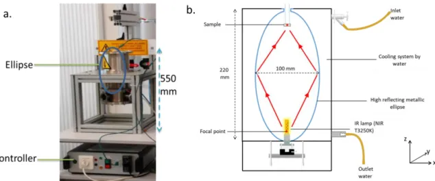
An existing heating device used previously for several applications like for example pyrolysis [42] has been modified for direct method based emissivity measurement application. This device (Figure 1) consists of an elliptical high reflecting stainless steel surface. A radiative source is located at one focal point of the ellipse while the sample stands at the other focal point. The sample temperature is monitored by a thermocouple and can be controlled either manually or using PID controller adjusting the lamp input power. Sample heating method by an elliptical furnace allows high heating rate, ramp temperatures, cycling and temperature bearing and its design allows to easily switch between different atmospheric conditions. The external walls of the ellipse are maintained at ambient temperature by circulating water whose temperature can be controlled. Water can also be easily replaced by liquid nitrogen on the cooling system.

This is the aut

ver, the online

from this

version

once it has bee

(10)

9

Figure 1 : Device original design: photograph (a), cross-section view (b)

In practice, the radiative source is significantly larger than a point and its accurate positioning at the focal point is challenging. Hence, a position adjustment system is added in order to allow translations of the lamp along x, y, and z axis. A rotation around x and y is also made possible in order to account for possible filament disorientations. The emission of the heated sample is then measured on its top (back) face using either a NIR spectrometer equipped with a high temperature resisting fiber optics or with IR cameras (through a tilted flat Ag mirror). A turbomolecular vacuum pump is available for the device allowing measurements under secondary vacuum environment.

2.2. Characteristics of the radiative source

As mentioned above, the light source geometry needs to be known precisely in order to estimate its projection at the image focal point and therefore to assess the incoming heat flux on the sample. For most commercial high power lamps, the filament geometry consists in a vertical spiral. Considering the present application, the choice naturally comes down to an IR high power halogen lamp with a long vertical double-coiled filament. The IR lamp used in this work is manufactured by USHIO®, has a nominal power of 1000W, a filament length of 25mm, a filament diameter of 4.5 mm and a nominal color temperature of 3200K. The maximum emission corresponding wavelength calculated is 906 nm. The choice for a high power lamp allows having a wide range of heating rate on the sample. An infrared image (Figure 2) of the filament is captured with a NIR [0.9-1.7] µm camera XENICS® Xeva equipped with a macro lens to evaluate the maximum emission area and to observe emission gradients along the filament length.

This is the aut

ver, the online

from this

version

once it has bee

(11)

10

Figure 2 : Lamp filament emission: photograph (a), infrared image (b), Normalized flux (c) It is seen in Figure 2 that the maximum emission area is located at the filament center and a maximal difference of 15% is observed between center and extremities of the filament. The difference is only of 5% in the four spires located at the center which corresponds at a length of 11 mm. Such dimensions improve the positioning flexibility of the sample with respect to the source. Indeed the illuminated zone in the vicinity of the image focal point is larger.

2.3. Design of the sample holder

2.3.1. Determination of sample dimensions

The optimum diameter of the sample is computed from a Ray Tracing technique as in reference [11] [43]. Indeed, the incoming irradiance over the sample needs to be as high as possible (to reach the target temperature of 1200°C), but above all, as homogeneous as possible. A first order approximation allows assessing the temperature of the sample from its response to a constant incoming flux on one side from:

𝑇(𝑡) = 𝑇₀+ 2𝑃𝐸

ℎ_𝑔𝜋𝑑2(1 − 𝑒

−_𝜏𝑡₎

(12)

Where 𝑇₀ is the initial sample temperature, 𝑑 the sample diameter, 𝑃_𝐸 the effective incoming flux on

the sample, ℎ𝑔 the global heat transfer coefficient, d the sample diameter and 𝜏 the time constant. It

therefore comes that the maximum temperature at steady state, is given by:

𝑇_𝑚𝑎𝑥= lim

𝑡→+∞𝑇(𝑡) = 𝑇0+

2𝑃_𝐸

ℎ_𝑔𝜋𝑑2 (13)

The global heat transfer coefficient ℎ𝑔 is approximated for the sum of the convective and radiative

exchange coefficients [44]. The Ray Tracing model is used to assess the effective incoming power 𝑃_𝐸

from the following equation:

𝑃_𝐸 = 𝑃_𝑛𝑜𝑚∙ 𝛼 ∙ 𝛽 (14)

Where 𝑃𝑛𝑜𝑚 is the nominal (input) power of the lamps, 𝛼 is the sample absorptivity and 𝛽 is the ratio

of the incoming flux on the sample over the lamp’s emitted flux and is defined as :

𝛽 =∑ 𝑃𝑠(𝑧) ∙ 𝜌𝑤 𝑟𝑖 𝑁_𝑡 𝑖=1 ∑𝑁_𝑖=1𝑡 𝑃𝑠(𝑧) (15)

where 𝑁𝑡 = 107 is the total number of computed rays, 𝜌𝑤 = 0.97 is the ellipse walls reflectance and

𝑟𝑖 stand for the number of reflections of the ith_{ray. Indeed, each ray leaves the lamp with a}

normalized power ranging from 0.75 to 1 according to the vertical positon 𝑧 of the starting point and

This is the aut

ver, the online

from this

version

once it has bee

(12)

11

the measured flux depicted in Figure 2. This power decreases after each reflection on the ellipse walls. In order to describe the possible heterogeneity of temperature over the sample, the power ratio 𝛽 can be discretized along the sample radius 𝑟 to compute the power ratio received at each

location. For this purpose, the sample radius is divided into 50 cells and 𝛽𝑗 is assessed from

𝛽_𝑗 =∑ 𝑃𝑠(𝑧) ∙ 𝜌𝑤 𝑟𝑖 𝑖∈𝑁𝑗 ∑_𝑖∈𝑁 𝑃_𝑠(𝑧) 𝑗 With 𝛽 = ∑ 𝛽_𝑗 50 𝑗=1 (16)

Where 𝑁𝑗 is the set of rays that hits the jth cell of the sample.

The lamp filament is modelled as a 25x4.5 mm2_{cylinder and the power assigned to each ray depends}

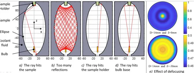
on its starting position along the z axis. Four cases are treated as depicted in Figure 3. The first case is the general case where the ray ends up on the sample after 𝑟𝑖 reflections, the second corresponds to a number of reflection leading to decrease the ray power below 10% of its initial value (i.e. 76

reflections with 𝜌𝑒𝑙𝑙𝑖𝑝𝑠𝑒 = 0.97), in the third and fourth cases, the ray hits either the sample holder

or the bulb base. In cases 2 to 4, 𝑟𝑖 is set to 𝑟𝑖 = +∞ i.e. the rays is discarded form the power computation.

Simple considerations lead to consider that the flux ratio 𝛽 depends on both the sample diameter and its vertical (z) position with respect to the focal point (denoted 𝛿). Indeed, as depicted in Figure 3e, the vertical shift 𝛿 from the focus point leads to flatten the flux (defocusing effect) and modify

the distribution of the 𝛽𝑗. Consequently, a total of 72 combinations of the sample positions (𝛿 =

[+5 ; −40]) and diameters (𝐷 = [10; 20]) are tested. A minimal diameter of 10mm is imposed by the necessity to weld a thermocouple on the sample back face and to get enough surface on the sample for optical measurement.

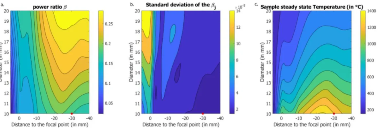
Figure 3: (a-d), ray tracing for several cases. (e) radial distribution of 𝜷_𝒋: defocusing effect Figure 4.a depicts the flux ratio 𝛽 for various diameters and vertical offsets, Figure 4.b it standard deviation along the radius of the sample (i.e. the flux homogeneity over the sample) and the Figure

This is the aut

ver, the online

from this

version

once it has bee

(13)

12

4c depicted the computed steady state temperature assessed from equation (13). α value is set at

0.5 and a hg value of 122.5 W.m-2.K-1 is computed [44].

Figure 4: Flux ratio for several configurations (a), flux homogeneity over the sample (b), computed steady-state temperature (c)

It is seen from Figure 4 that increasing the sample diameter is not relevant. Indeed it leads to decrease the temperature with no gain on the spatial homogeneity of the incoming flux. In addition, defocusing of 10mm to 30mm significantly strengthen the homogenous flux hypothesis. Accordingly, in the following, a sample diameter of D=10mm and a distance to the focal point of δ=-30mm are chosen.

2.3.2. Sample holder characteristics

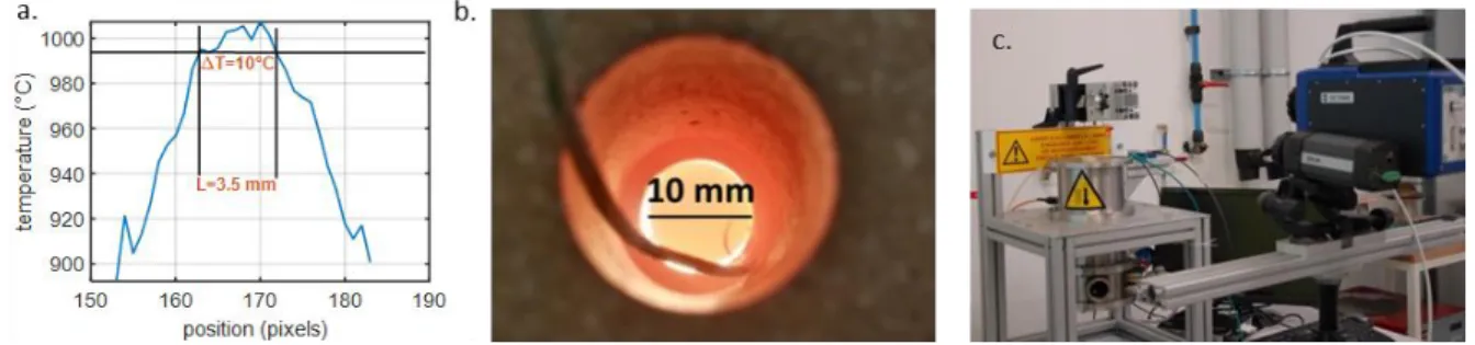
A sample holder is required to position and maintain the sample within the cavity. The main expected characteristics are a good resistance to high temperatures (1200°C), a low thermal conductivity (to decrease thermal gradients within the sample), a low thermal expansion coefficient and optical opacity (to avoid radiation lamp interference on the measured face of the sample). The material selected to abide by those conditions is a soapstone refractory ceramic. The sample holder is designed to center a 10 mm diameter sample equipped with a thermocouple. Ceramic wedges are used to set precisely the vertical position of the sample. As an example to validate heating performances, a platinum sample put on the optimal position defined in 2.3.1 part is heated with the IR lamp power set at 100%. The sample reaches a maximal temperature of 1100°C at a rate of 8°C/s. In Figure 5, temperature gradient across the sample are depicted for a targeted temperature of 1000°C (measurement are made using a BII FLIR SC7000 MIR camera). The tolerable gap between the maximum and the minimum temperature of the measuring zone is set to 10°C. Therefore, a 3.5 mm diameter circular maximal area is defined as the emissivity measurement zone.

This is the aut

ver, the online

from this

version

once it has bee

(14)

13

Figure 5 : Temperature gradient on the sample: experimental set-up (a), photograph of the heated sample (b), maximal area defined for emissivity measurement (c)

In this section, the requirements of the measurement have been achieved thanks to a numerical Ray Tracing approach, confirmed by experimental measurements. The diameter of the sample, the position to the focus point and the ability to reach a temperature of 1100°C have been demonstrated. Sample Temperature Dimension Optimal Position Sample holder material Maximal value Heating rate 10 mm diameter 30 mm from

focal point Soapstone 1100 °C 8°C/s

Table 3 : Defined sample characteristics and temperature attainments

3. Calibration and instrumentation of the system

3.1. Selection of the sensors for a wide band detection

The measurement of spectral emissivity from direct method requires the most suited selection of sensors as implied by Wien’s displacement law (eq.1). Moreover, as mentioned above, the hot forming applications targeted in the present paper lead to focus on temperature range [600-1000]°C. The blackbody radiation calculated by Planck’s law and their corresponding derived curves for these temperatures are shown in Figure 6.

This is the aut

ver, the online

from this

version

once it has bee

(15)

14

Figure 6 : Blackbody emission (a) and derived curves (b)

For temperatures of 600°C and 1000°C, wavelengths corresponding to maximum emission are respectively found at 2.26 and 3.31µm which implies emitted radiations respectively between [1.13-11.3] µm and [1.65-16.5] µm. Therefore, investigating integrated emissivity requires the whole classical ranges of IR sensors: namely band I for NIR, and bands II and III for MIR. The derived curves depicted in Figure 6.b) show the high sensitivity of NIR BI wavelengths at high temperature and conversely the low sensitivity for MIR BIII. An optimal emissivity measurement would be done through a continuous sensor operating between 1.1 and 16.5 µm. However, the device requirement for standalone measurements and the sensors availability dictate a discontinuous measurement between 1.3 and 10 µm. The design device still allows to easily change sensors with thermopile, photodiode…

For NIR measurements, a FT-IR spectrometer NeoSpectra® operating at [1.3; 2.5] µm equipped with a single PbS photodetector is used. The spectrometer input plug is connected to a high temperature resistant optical fiber that is put very close to the sample (less than 3mm). This fiber can operate between -20 and 1000°C. For MIR BII measurements, an IR camera FLIR SC7000 equipped with a filter wheel is used. This camera has a resolution of 320*256 pixels with an image frequency from 1 to 500 Hz. Integration time can be adjusted between 1 µs to around 1s. Its spectral range spreads from 2.5µm to 5.5µm. The sensor is also cooled by an internal stirling system. For MIR BIII measurements, an IR camera FLIR SC325 is used. This camera has a resolution of 320*240 pixels with an image frequency of 30Hz and a spectral range between 7.5 and 13µm. BII and BIII cameras will be equipped with filters described in Table 4.

Camera MIR BII MIR BIII

Wavelength (µm) 3,027 4 5,071 10

Bandwidth (nm) 60 80 96 2000

Transmission at

peak (%) 73.91 60 68.86 92

Table 4 : Optical filters characteristics

MIR BII filters wavelengths are selected to have a regular distribution on the SC7000 camera bandwidth with three bandpass filters allowing measurements respectively at the beginning, the center and the end of the camera bandwidth. For MIR BIII measurements, a sole bandpass filter with

This is the aut

ver, the online

from this

version

once it has bee

(16)

15

a wavelength corresponding at SC325 camera bandwidth center is selected. The discontinuity on the measurement caused by this filter selection will then be studied in part 3.2.

3.2. Influence of spectrum discontinuity on integrated emissivity

The goal of the presented experiment is to provide both spectral emissivity and integrated emissivity. In practice, the integrated emissivity is calculated from the spectral emissivity measurement. However, such computation usually relies on the hypothesis of radiance continuity over the emission spectrum which can hardly be satisfied with the sensors selection presented in section 3.1.

Accordingly, the discontinuities of the obtained spectrum lead to an integration error on the integrated emissivity value. It is here proposed to assess such error from the comparison of integrated emissivity calculated from continuous or discontinuous spectrums. The chosen reference material is polished Platinum for which the spectral normal emissivity can be calculated from its optical indices [45] and the radiative properties slightly depends on temperature. Figure 7 shows the obtained continuous spectrum, the detection bands of the NIR spectrometer and the camera filters bands are also highlighted. The missing points in-between these bands are interpolated using either linear, cubic or Akima splines interpolant[46]. The corresponding emissivity spectrums are then integrated using (6) and compared to the continuous integration (see Table 5), with the Platinum spectral emissivity chosen at room temperature.

Figure 7: Theoretical spectral emissivity for polished platinum [45] and interpolated values with linear, cubic and Akima spline interpolant

In is seen from Table 5 that the integrated emissivity calculated from the Akima spline interpolant exhibits lower errors than other approaches and remains always below 0.2%. Accordingly this latter interpolation will be used in the present study.

Another significant source of error is the bounds of the integration. Indeed the chosen sensor impose the integration over 1.3µm to 11µm while the bound of Eq.6 are 0 and +inf. Using the data proposed by Palik et al. [45], the discrepancy between the two integrated values of emissivity can be assessed to 4.7% and 0.37% for 600°C and 1000°C respectively. At the lowest temperature, the error mainly comes from the far infrared cut-off (at 10µm with the proposed setup). Such drawback can be tackle

This is the aut

ver, the online

from this

version

once it has bee

(17)

16

down be adding another sensor above 10µm. For instance, the error comes down to 1.8% at 600°C with an extra point at 14µm.

Spectrum Palik [45] Linear

interpolant Cubic interpolant Akima spline interpolant T=600°C ε 0.0746 0,0773 0,0750 0.0747 Δε/ε (%) - 3,8 0,59 0.10 T=1000°C ε 0.1185 0.1211 0.1192 0.1187 Δε/ε (%) - 2.1 0.33 0.17

Table 5 : Integrated emissivity calculation with continuous and discontinuous spectrums To sum up, in this section, the choice of an optimized interpolation method (Akima spline interpolant) has been performed to compensate the use of spectral detectors and not total radiation ones. However, at low temperatures, the main source of error is the maximum detection wavelength of the system (11µm), which is below the maximum emission wavelength of thermal emission.

3.2. Thermal calibration of sensors

3.2.1. Thermal calibration

o Thermal calibration of the NIR spectrometer

The spectrometer (equipped with an optical fiber (see section 2.)) is calibrated between 600 and 1000°C using a R1500T Land blackbody. Corresponding spectrums are represented in Figure 8.

Figure 8 : NIR spectrometer calibration with primary blackbody

Spectrum values increase with temperature and a peak is observed at 2.2µm corresponding to the maximum spectral response of the photodetector. Emitted blackbody signal is multiplied by the photodetector spectral response and the fiber transmission which explained the curves’ shape.

o Thermal calibration of the MIR camera SC7000

MIR camera equipped with three filters (around 3, 4 and 5 µm) is calibrated for each configuration

(Figure 9a.). To avoid saturation, a signal value (Id) of 10000 digital levels is maintained by adjusting

integrating time (ti). Ratio between digital levels under exposition time increases with temperature.

For a monochromatic case, this ratio is supposed to decrease with wavelength unlike what is shown in Figure 9a. This shift can be explained by the difference of bandwidth and maximum transmission at peak between each filter (Cf. Table 4).

This is the aut

ver, the online

from this

version

once it has bee

(18)

17 o Thermal calibration of the MIR camera SC325

Unlike SC7000 camera, exposition time is not adjustable on BIII camera SC325. Digital levels (b.) with a 10µm filter equipped on camera present a linear trend which implies a quasi-constant sensitivity with temperature over this range (see section 3.1). This trend seems in opposition with Planck’s law, but this is only a scale effect. Enlarging the temperature range would lead to the classical exponential rise as seen in Figure 9 a.

Figure 9 : a. MIR BII SC7000 camera calibration with blackbody, b. MIR BIII SC325 camera calibration with blackbody

3.2.2. Measurement uncertainties

Among the influence quantities governing the emissivity uncertainty (sensor noise, spurious signal, temperature uncertainty, sample thermal heterogeneity…), thermal effects are dominating. In this section, the uncertainty arising from a non-uniform temperature distribution over the sample and on the temperature measured value due to sensor uncertainty are investigated.

o Effect of non-uniform temperature distribution

Preliminary, this problem does not concern the MIR BII and BIII measurements, as they are performed using infrared cameras. Indeed, the thermal homogeneity of the surface over the projection of one pixel on the sample (around 500µm) can be considered as satisfactory (see Fig. 2). On the contrary, the BI measurement performed by the means of an optical fiber with a nonzero acceptance cone must be discussed. The measurement is here performed on a small surface, with a possible thermal gradient on it, and the sensor integrates spatially the signal over such elementary surface

The optical fiber has an acceptance angle of 30° and is put very close to the sample surface (2.5 mm), which implies a 1.38 mm diameter area for the measurement. According to Figure 5, the

corresponding temperature gap is ΔT=3°C (i.e. σT=1°C for a Gaussian distribution). Uncertainty on

emissivity measurement arising from non-uniformity temperature can be evaluated through the following formula[47] :

This is the aut

ver, the online

from this

version

once it has bee

(19)

18 Δε 𝜀 (𝑁𝑈) = | 𝑐₂/(𝜆𝑇) exp (−_𝜆𝑇𝑐2) − 1| Δ𝑇 𝑇 (17)

This equation can also be written with standard deviations (Δε=3*σε and ΔT=3*σT) for a Gaussian

distribution. This relative standard deviation is presented between 1 and 16.5µm in Figure 10.

Figure 10 : Relative standard deviation on emissivity measurement arising from non-uniformity temperature between 1 and 16.5 µm for a 3°C temperature gap

Non uniformity temperature has a higher impact on emissivity measurement in NIR range and lower in MIR range. It is also shown that the uncertainty on emissivity decreases slightly with temperature. The highest error is then recorded on the edges of the measurement area and is maximum at 600°c, but remains inferior to 1.3% on the NIR spectrometer range and lower than 0.3% on the MIR range.

o Effect of temperature uncertainty (TU) on emissivity

In this work, the emissivity is calculated by a direct method, and is defined as the ratio of the

detector signals S(T) to the black body signal (S0(T) set at the same temperature T). Hence, a bias on

the temperature impacts the signals detected, so the emissivity evaluation, as depicted by the following formula:

σ_𝜀

𝜀 (𝑇𝑈) = 2 ∗

σ_𝑆

𝑆 (18)

In order to link the signals and the temperature uncertainties, it is necessary to introduce the sensitivity of the detector, denoted k(T). This study is performed at wavelength 2.2µm for NIR spectrometer and 5.071µm for MIR BII camera, where sensitivity is maximum for each band, in order to maximize the uncertainty. . Moreover, as the NIR BI and MIR BII detectors response are non-linear, the sensitivity depends on the temperature, and the detectors response is approximated by a second-order polynomial (as the analytical formula is unknown).On the other hand, MIR BIII detector’s response is approximated by a linear approximation. Temperature sensitivity is then deduced from raw signal spectrums.

Signal uncertainty can then be deduced from sensitivity and sensor uncertainty following this formula (for small variations of the temperature):

σ_S(T) = k(T) ∗ σ_T (19)

Where k is the temperature sensitivity (A.U. °C-1_{), 𝜎}

𝑆 the signal standard deviation (A.U).

This is the aut

ver, the online

from this

version

once it has bee

(20)

19

The absolute error on temperature ΔT is fixed by the chosen sensor (type K thermocouple). For such device, the manufacturer standard claims that the deviation evolves linearly in between 333 and 1200°C:

σ_T= 0.0025 ∗ T (20)

To sum up, the relative uncertainty on emissivity is given by the following formula:

σ_𝜀

𝜀 (𝑇𝑈) = 2 ∗

0.0025 ∗ k(T) ∗ T

𝑆 (𝑇) (21)

To finish, the total uncertainties are obtained by the propagation of the standard deviations deduced from each cause of error, applying a coverage factor of 2.

σ_𝜀

𝜀 (𝑇𝑈) = 2 ∗

0.0025 ∗ k(T) ∗ T

𝑆 (𝑇) (22)

Table 6 presents the maximum total uncertainty for each spectral band.

Detector’s range NIR BI MIR BII MIR BIII

Wavelength (µm) 2.2 5.071 10

Approximated detector’s

response (A.U) 2 ∗ 10

−6_{∗ 𝑇}2_{− 0.0022 ∗ 𝑇 + 0.63} _{0.0011 ∗ 𝑇}2_{− 0.27 ∗ 𝑇 − 149.2} _{42 ∗ 𝑇 − 960}

Sensitivity (A.U.°C-1₎ _{𝑘(𝑇) = 4 ∗ 10}−6_{∗ 𝑇 − 0.0022} _{𝑘(𝑇) = 0.0022 ∗ 𝑇 − 0.27} _{𝑘(𝑇) = 42}

Maximal uncertainty (%) 7.4 (at 700°C) 1.3 (at 600°C) 1.5 (at 600°C)

Table 6 : Relative emissivity uncertainties arising from temperature uncertainty

Uncertainties due to non-uniform temperature distribution and temperature uncertainty are only relevant in NIR BI measurements. Indeed, uncertainties due to temperature do not exceed 1.5% in MIR BII and MIR BIII. Maximum combined uncertainties due to temperature effects in NIR band are observed at 700°C with a value of 7.4%. However, this maximal uncertainty slightly decreases with temperature with a value of 5.4% at 1000°C.

3.2.3. Sample-holder contribution on the measurement

As depicted in Figure 11 the chosen setup imposes to have the sample positioned into a sample-holder that absorbs a part of the flux emitted by the lamp and is also heated by the sample through thermal conduction. Accordingly, the sample holder own emission interferes with the measurement. Such emission can be spitted in three contributions as follows:

𝑆̃(𝑇) = 𝑆(𝑇) + 𝑆_𝑠ℎ1(𝑇𝑠ℎ, Ω1) + 𝜌(𝑇)𝑆𝑠ℎ2(𝑇𝑠ℎ, Ω2) + 𝑆𝑙+ 𝑆𝑑 (23)

Where 𝑆_𝑠ℎ1 is the emitted signal toward the sensor (Ω₁being the viewing solid angle of the sample

holder from the sensor), 𝑆𝑠ℎ2 is the signal emitted from the sample-holder and reflected upon the

sample surface ((Ω2 is then the viewing solid angle of the sample from the sensor) and 𝑆𝑠ℎ3 is the

complementary part of the emitted flux from the sample holder so that Ω = Ω1+ Ω2+ Ω3= 2𝜋 𝑠𝑟.

This is the aut

ver, the online

from this

version

once it has bee

(21)

20

Consequently, the signal received by sensors 𝑆̃(𝑇) (i.e. the measurement) is a sum of various contribution among which the emitted signal from the sample 𝑆(𝑇), spurious signal emitted from the

sample-holder 𝑆_𝑠ℎ1(𝑇_𝑠ℎ), the reflection of this latter emission over the sample surface 𝜌𝜆(𝑇) ∗

𝑆_𝑠ℎ2(𝑇_𝑠ℎ) (where 𝜌 stands for the sample reflectance), the signal leaked by the lamp through

sample-holder gaps 𝑆𝑙 and the intrinsic sensor signal 𝑆𝑑 (detector offset). All those spurious signals,

(summarized in Eq. 23) must be assessed to access the intended measure 𝜀(𝑇) from 𝑆̃(𝑇).

One should notice that this equation reads differently for the two setups discussed in the above: the NIR configuration where an optical fiber is used and the MWIR configuration where an Ag mirror is used.

Figure 11 : Spurious signals illustration for: NIR configuration (a), MIR configuration (b)

When placed in front of a cavity blackbody set at a temperature 𝑇, the contribution of the sample

holder is obviously null along with the spurious direct signal from the lamp 𝑆_𝑙. The measurement

reads:

𝑆̃0_{(𝑇) = 𝑆}0_{(𝑇) + 𝑆}

𝑑 (24)

Which allows the assessment of 𝑆0(𝑇). Hence, equation (23) can be rewritten by replacing sample

signal 𝑆(𝑇) by the product of spectral emissivity and blackbody emission 𝑆0_(𝑇)_{using Equation 2.}

𝑆̃(𝑇) = 𝜀(𝑇)𝑆0(𝑇) + 𝑆_𝑠ℎ1(𝑇_𝑠ℎ) + 𝜌(𝑇)𝑆_𝑠ℎ2(𝑇_𝑠ℎ)+ 𝑆_𝑙+ 𝑆_𝑑 (25)

Kirchhoff’s law, applied to opaque materials, enables to link the emissivity to reflectivity as ε=1-ρ. Eq.25 becomes: 𝑆̃(𝑇) = 𝜀(𝑇)𝑆0(𝑇) + 𝑆𝑠ℎ1(𝑇𝑠ℎ) + (1 − 𝜀(𝑇))𝑆𝑠ℎ2(𝑇𝑠ℎ)+ 𝑆𝑙+ 𝑆𝑑 (26) And 𝜀(𝑇) =𝑆̃(𝑇) − 𝑆𝑠ℎ1(𝑇𝑠ℎ) − 𝑆𝑠ℎ2(𝑇𝑠ℎ) − 𝑆𝑙− 𝑆𝑑 𝑆0₍_𝑇_{) − 𝑆} 𝑠ℎ2(𝑇𝑠ℎ)

This is the aut

ver, the online

from this

version

once it has bee

(22)

21

The variables 𝑆_𝑠ℎ1(𝑇_𝑠ℎ), 𝑆_𝑠ℎ2(𝑇_𝑠ℎ), 𝑆_𝑙 and 𝑆_𝑑 can be phrased as the contributions of all unintended

emissions from the environment. Their evaluations depend on the selected setup (NIR or MWIR). 𝑆_𝑠ℎ1(𝑇_𝑠ℎ), and 𝑆_𝑠ℎ2(𝑇_𝑠ℎ)contributions on the measurement can be either computed by numerical simulation or evaluated experimentally. Nevertheless, boundary limits (sample holder temperature, sample temperature distribution, radiative properties) need to be known precisely for numerical computation. An experimental evaluation seems more appropriate and simpler for this set-up.

o Environment contribution in NIR BI

The use of the NIR spectrometer involves an optical path through an optical fiber. It has an acceptance angle of 30° and is put very close (2.5 mm) to the sample surface. The projected measure therefore covers a 1.44 mm radius circle, hence fully included upon the sample surface. Accordingly,

spurious signals originating from both the lamp (𝑆𝑙) and the direct emission of the sample-holder (

𝑆𝑠ℎ1(𝑇𝑠ℎ)) can be neglected and discarded. It therefore comes:

𝜀(𝑇) =𝑆̃(𝑇) − 𝑆𝑠ℎ2(𝑇) − 𝑆𝑑 𝑆0₍_𝑇_{) − 𝑆} 𝑠ℎ2(𝑇) = 𝑆̃(𝑇) − 𝑆𝑠ℎ2(𝑇) − 𝑆𝑑 𝑆̃(0 _𝑇_{) − 𝑆} 𝑠ℎ2(𝑇) − 𝑆𝑑 (27)

𝑆_𝑑 can be easily assessed from shielding the optical fiber from any incoming flux within its operating

wavelength range. On the other hand, assessing 𝑆_𝑠ℎ2(𝑇) requires a specific setup. Rewriting Eq.26 it

comes:

𝑆_𝑠ℎ2(𝑇) =(𝑆̃(𝑇) − 𝑆𝑑) − 𝜀(𝑇) ∗ (𝑆

0

̃(𝑇) − 𝑆_𝑑)

1 − 𝜀(𝑇) (28)

Therefore, a reference material whose emissivity is known precisely can be used to assess this sample holder signal contribution. This material has to be highly reflective to minimize direct signal emitted by the sample and ideally must have low emissivity variations with temperature. Polished platinum fills those conditions considering its chemical stability and low oxidation with temperature. Furthermore, the low dependence of emissivity platinum with temperature in NIR band has been shown (1.8 to 3.1µm for this work) by Deemyad and Silvera [48]. This statement is also confirmed by CEMHTI [34] in their works on platinum χ point. Under the hypothesis of a constant emissivity with temperature (𝜀(𝑇) ≈ 𝜀(20°𝐶)), the emissivity of a polished platinum sample is measured at room

temperature on a commercial IRTF spectrometer Bruker vertex 70 with the help of an infragold

integrating sphere. This value is then used in Eq.28 to assess 𝑆𝑠ℎ2(𝑇). Figure 12a depicts the

evolution of such contribution with respect to temperatures 𝑇 ranging from 600°C to 1000°C.

This is the aut

ver, the online

from this

version

once it has bee

(23)

22

Figure 12 : Spurious sample holder signal spectrums (a) and comparison with platinum sample emission at 1000°C (b)

Sample-holder emission increases with temperature and corresponding signal curves have the same shape than the sample’s one. The Figure 12b also shows that this spurious contribution cannot be overlooked especially at high temperature with a value close to 50% of the signal emitted by the sample at 1000°C.

o Environment contribution in MIR BII and BIII

In this configuration, the cavity of the sample-holder is empty allowing any spurious signal to reach the sensor. It is chosen to use a cooled metallic pipe to discard the contributions of the sample

holder and the lamp 𝑆𝑠ℎ1= 𝑆𝑙 = 𝑆𝑠ℎ2 = 0. In practice, the pipe needs to be cooled in order to

prevent any emission from it. Therefore, once the targeted temperature of the sample is reached, the pipe is inserted and for a short period of time (around 3 seconds), the measured signal becomes:

𝑆̃(𝑇) =𝜀(𝑇)𝑆0₍_𝑇_{) + 𝑆} 𝑑 ⇒ 𝜀(𝑇) = 𝑆̃ − 𝑆_𝑑 𝑆0 = 𝑆̃ − 𝑆_𝑑 𝑆̃ − 𝑆0 𝑑 (28) Such approach implies a fast insertion of the pipe (around 1 second) and an instant measure afterward to avoid a new spurious signal arising from the pipe as it heats up.

4. Results

4.1. Sample characteristics and experiment set up

o Sample characteristics

Two platinum samples are used in the present paper. Sample A is used for environment influence computation and Sample B is used for device validation. Both exhibit a commercial purity of 99.95%. The sample A is polished with a 2µm felt in order to increase its reflectance and then improve the environment influence calculation (cf. Eq.28). The sample B is processed as-received. Roughness measurements were made on both samples and are presented in Table 7. The value of Sa and Sq are presented along with the classical roughness Ra and Rq since they provide valuable information on the surface flatness (absent from the Ra and Rq calculations).

This is the aut

ver, the online

from this

version

once it has bee

(24)

23

Dimensions Waviness &

Roughness Roughness Diameter (mm) Thickness (mm) Biot number at 1000°C Sa (µm) Sq (µm) Ra (µm) Filter .8mm Rq (µm) Filter .8mm Sample A 10 1.5 0.0003 1.09 1.38 0.253 0.412 Sample B 10 2.5 0.0004 2.10 3.03 1.08 1.41

Table 7 : Waviness and roughness values o Experimental set-up

Emissivity measurement is done in three phases: NIR BI with the spectrometer described in part3, MIR BII with SC7000 FLIR camera and MIR BIII with SC325 FLIR camera. Platinum samples temperature is measured by a 0.3 mm diameter K type welded thermocouple protected with ceramic rings, which is also used for temperature regulation. For NIR BI measurements, optical fiber position is held by a fiber holder to ensure repeatability of the measurement. Optical fiber head position is set at 2.5 mm of the sample surface. The Ag mirror used for BII and BIII measurement exhibit an average reflectance of 0.95 over [1µm – 14µm]. A stainless steel pipe is inserted once the sample temperature is stable in order to assess and remove parasitic signals (see section 3.3.2).

Figure 13: Experimental set-up for emissivity measurement: cross-section view (a), photograph (b)

4.2. Spectral emissivity measurement

o NIR BI measurements

Platinum spectral emissivity in the NIR range is presented in Figure 14a. Low dependence of spectral emissivity with temperature can be seen which is confirmed by several works ([34], [48]). Spectral emissivity seems to follow two different trends: up to 1.8µm its value is quasi-constant then a regular decrease is observed afterward. The obtained spectra are compared to a measurement performed at 25°C using spectrometer Bruker vertex 70 (Figure 15) through an integrating sphere and an InGaAs photodetector (Figure 14b.). The emissivity error in this spectral range can then be estimated computing the relative error between the measurement performed on the apparatus and the one performed by the reference spectrometer at room temperature.

This is the aut

ver, the online

from this

version

once it has bee

(25)

24

Except for the measurement at 600°C, the calculated errors remain low in this spectral range. Error is decreasing when temperatures increases which can be explained by a more favorable signal-to-noise ratio at high temperature. Alike spectral emissivity, error seems to follow two trends: until 2µm its value is quasi-constant and lower than 5% and a regular increase can be observed after this value. This can be explained by the loss of efficiency for the detector InGaAs in this range. Error value is highest at 2.5µm which corresponds to the end of the spectrometer’s spectral range.

Figure 14 : NIR platinum spectral emissivity (a), relative error compared to reference measurement (b)

o MIR BII and BIII measurements

Platinum spectral emissivity values in the MIR BII and BIII bands are presented in Table 8. Unlike measurements in NIR BI, measurements in BII are done for specific wavelengths corresponding to camera’s filters described in part 3.1. Alike in the NIR range, emissivity presents a low variation with temperature. Those values are compared to a measurement done through the emission adapter of spectrometer Bruker Vertex 70 equipped with a DLaTGS detector at 400°C.

Figure 15 : IRTF spectrometer Bruker Vertex 70 with integrating sphere and emission adapter equipped

Emissivity values measured on the MIR BII are very close to the reference value except for emissivity value at 5.071 µm which present a shift between 700°C and 1000°C but the low value of emissivity at this wavelength induces a high error on measurement. Emissivity measurements on the MIR BIII

This is the aut

ver, the online

from this

version

once it has bee