Increasing the energy yield of generation from new and renewable energy resources

HAL Id: hal-01848950

https://hal.archives-ouvertes.fr/hal-01848950

Submitted on 25 Jul 2018

HAL is a multi-disciplinary open access

archive for the deposit and dissemination of

sci-entific research documents, whether they are

pub-lished or not. The documents may come from

teaching and research institutions in France or

abroad, or from public or private research centers.

L’archive ouverte pluridisciplinaire HAL, est

destinée au dépôt et à la diffusion de documents

scientifiques de niveau recherche, publiés ou non,

émanant des établissements d’enseignement et de

recherche français ou étrangers, des laboratoires

publics ou privés.

Increasing the energy yield of generation from new and

renewable energy resources

Samuel C. E. Jupe, Andrea Michiorri, Philip C. Taylor

To cite this version:

Samuel C. E. Jupe, Andrea Michiorri, Philip C. Taylor. Increasing the energy yield of generation from

new and renewable energy resources. Thomas Hammons. Renewable Energy, IntechOpen, pp.37-62,

2009, 978-953-7619-52-7. �10.5772/7379�. �hal-01848950�

Increasing the energy yield of generation from

new and renewable energy resources

Samuel C. E. Jupe, Andrea Michiorri, Philip C. Taylor,

Durham University, UK

1. Introduction

The impetus of governments, on an international scale, to move towards low-carbon economy targets has brought about the proliferation of electricity (and heat) generation from new and renewable energy (RE) resources. This, coupled with increasing consumer energy demands, has caused distribution network operators (DNOs) to seek methods of increasing the utilisation of their existing power system assets. The increased utilisation of assets must be realised cautiously such that the security of supply to customers is not reduced, particularly when the age of distribution network assets is taken into account. A developer that is seeking to connect generation of significant capacity may be offered a firm connection by the DNO on the condition that an investment is made (by the developer) in the necessary network reinforcements. However, the developer may not be able to justify the expense of the required reinforcement and may negotiate a non-firm or „constrained‟ connection agreement, whereby the generation installation is tripped off or constrained back under certain network operating conditions. Furthermore, difficulties may be encountered when attempting to gain permission to build network infrastructure, in order to accommodate new generation installations, due to planning problems and environmental objections (Fox-Penner, 2001). One potential solution or means of deferring these problems is the adoption of real-time thermal rating systems which have the potential, in certain circumstances, to be both less invasive and more cost effective when compared to network reinforcement options. Non-firm generation connections are expected to occur more frequently as network power flow congestion occurs. Therefore the deployment of a power output control system, informed by real-time thermal ratings, may be required to increase the energy yield of generation from new and RE resources.

The stages in the development of an output control system for generation installations are illustrated. Section 2 provides a comprehensive literature review in order to provide the context for the research presented. Section 3 describes the assessment of the location of power flow congestion within the power system (due to the proliferation of generation from new and RE resources) so as to facilitate the targeted development of thermal models for thermally vulnerable components. This is achieved through the calculation of thermal vulnerability factors that relate power flow sensitivity factors (derived from governing alternating current power flow equations) to component steady-state thermal limits. Section 4 describes models for the steady-state assessment of power system component real-time thermal ratings. Industrial standard lumped parameter models are described for overhead lines, electric cables and power transformers. In a consistent manner, these models allow the influence of environmental conditions (such as wind speed) on component real-time thermal ratings to be assessed. Section 5 describes thermal state estimation techniques that allow the rating of components, which are not directly monitored within the power system, to be assessed. Thermal state estimations facilitate the precise and reliable assessment of environmental conditions whereby a minimal number of meteorological monitoring allows the thermal state of components within a wide area to be

assessed. This may then be validated through the carefully selected monitoring of component operating temperatures. In Section 6, the power flow sensitivity factors are brought together with component real-time thermal ratings and candidate strategies are presented for the power output control of single or multiple generation installations. In Section 7, a case study is used to illustrate the developmental stages described above. In Section 8 the strengths and weaknesses of the proposed output control system for generation installations are discussed.

The research described in this chapter forms part of a UK government part-funded project (Neumann

et al, 2008) which aims to develop and deploy an online power output controller for wind generation

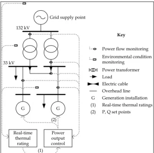
installations through the exploitation of component real-time thermal properties. This is based on the concept that high power flows resulting from wind generation at high wind speeds could be accommodated since the same wind speed has a positive effect on component cooling mechanisms. In this project the control system compares component real-time thermal ratings with network power flows and produces set points that are fed back to the generation scheme operator for implementation, as shown in Fig. 1. G G Real-time thermal rating Power output control

Power flow monitoring Environmental condition monitoring Power transformer Load Electric cable Overhead line 132 kV 33 kV Key

Grid supply point

P, Q set points Real-time thermal ratings

(1) (2)

(2) (1)

G Generation installation

Fig. 1 Generation power output controller informed by real-time thermal ratings

2. Background

Installed capacity assessments for generation from new and RE resources are the current research focus of numerous institutions in order to determine the impact of voltage regulations, operational economics, fault levels, losses and thermal limits as constraining parameters. Voltage limitations and the wind farm installed capacity relative to the system fault level in 33kV networks are considered (Dinic et al., 2006) and it is concluded that capacitive compensation can allow capacity maximisation within operational limits. The economics of generation connections to exploit multiple new and RE resources are considered (Currie et al., 2006) with a methodology that facilitates greater generation installed capacities. In order to manage power flows within prescribed voltage and thermal limits, operating margins are utilised with an active power output control technique termed „trim then trip‟.

An optimal power flow (OPF) technique is developed (Vovos et al., 2005) along with an iterative procedure to calculate the possible installed capacity of generation at nodes based on fault level limitations. The impact of increased generation installed capacities on electrical losses within the IEEE 34-node test network is examined (Mendez Quezada et al., 2006) and it is concluded that losses follow a U-shaped trajectory when plotted as a function of the generation penetration. An OPF formulation is presented (Harrison & Wallace, 2005) to determine the maximum generation installed capacity based on thermal limits and statutory voltage regulation. The „reverse load-ability‟ methodology coupled with OPF software models generators as loads with a fixed power factor and creates an analysis tool that could allow additional constraints (such as fault-level limitations) to be incorporated into the formulation if necessary.

Significant research has been carried out at the transmission level for real-time thermal rating applications. Research tends to focus on overhead lines which, due to their exposure to the environment, exhibit the greatest rating variability. A description of the cost and suitability of different uprating techniques for overhead lines is described (Stephen, 2004) taking into account different operating conditions. This work shows how real-time thermal ratings can be a more appropriate solution than network reinforcement when connecting new customers to the network who are able to curtail their generation output or reduce their power demand requirement at short notice. Similarly, experience regarding thermal uprating in the UK is reported (Hoffmann & Clark, 2004) where it was suggested that real-time thermal ratings could give overhead lines an average uprating of 5% for 50% of the year. An example of a real-time thermal rating application for transmission overhead lines of Red Eléctrica de España is described (Soto et al., 1998) where a minimal amount of weather stations are used to gather real-time data. The data is then processed using a meteorological model based on the Wind Atlas Analysis and Application Program (WAsP), taking into account the effect of obstacles and ground roughness, and the thermal rating is calculated. A similar system was developed in the USA by EPRI (Douglass & Edris, 1996) which considered overhead lines, power transformers, electric cables and substation equipment. Preliminary results of field tests (Douglass et

al., 1997) show that up to 12 hours of low wind speeds (<0.76 ms-1) were observed during the field tests which therefore suggests that overhead line real-time thermal ratings may be lower than seasonal ratings for extended periods of time. Furthermore, a strong correlation was found to exist between independent air temperature measurements distributed along the lengths of the overhead lines. At the distribution level, a real-time thermal rating project carried out by the Dutch companies NUON and KEMA (Nuijten & Geschiere, 2005) demonstrates the operating temperature monitoring of overhead lines, electric cables and power transformers.

The advantages of a real-time thermal rating system for the connection of generation from new and RE resources are reported in various sources, each of which considers only single power system components. It is demonstrated (Helmer, 2000) that the rating of transformers positioned at the base of wind turbines may presently be oversized by up to 20%. Moreover, the power flowing in an overhead line close to a wind farm is compared to its real-time thermal rating using WAsP (Belben & Ziesler, 2002). In this research it was highlighted that high power flows resulting from wind generation at high wind speeds could be accommodated since the same wind speed has a positive effect on the line cooling. This observation makes the adoption of real-time thermal rating systems relevant in applications where strong correlations exist between the cooling effect of environmental conditions and electrical power flow transfers. Moreover, the influence of component thermal model input errors on the accuracy of real-time thermal rating systems is studied (Piccolo et al., 2004; Ippolito et al., 2004; Villacci & Vaccaro, 2007). The application of different state estimation techniques, such as affine arithmetic, interval arithmetic and Montecarlo simulations was studied for overhead lines, electric cables and power transformers. Errors of up to ±20% for an operating point of 75oC, ±29% for an operating point of 60oC and ±15% for an operating point of 65oC were found

when estimating the operating temperature of overhead lines, electric cables and power transformers respectively. This highlights the necessity to have reliable and accurate environmental condition monitoring. The thermal models, used to estimate real-time thermal ratings for different types of power system components, are fundamental to this research as the accuracy of the models influence significantly the accuracy of real-time thermal ratings obtained. Particular attention was given to industrial standards because of their wide application and validation both in industry and academia. For overhead lines, the models (House & Tuttle, 1959; Morgan, 1982) have been developed into industrial standards by the IEC (IEC, 1995), CIGRE (WG 22.12, 1992) and IEEE (IEEE, 1993). Static seasonal ratings for different standard conductors and for calculated risks are provided by the Electricity Network Association (ENA, 1986). Thermal model calculation methods for electric cable ratings are described (Neher & McGrath, 1957) and developed into an industrial standard by the IEC (IEC, 1994). The same models are used by the IEEE (IEEE, 1994) and the ENA (ENA, 2004) to produce tables of calculated ratings for particular operating conditions. Power transformer thermal behaviour is described (Susa et al., 2005) with further models described in the industrial standards by the IEC (IEC, 2008), the IEEE (ANSI/IEEE, 1981) and the ENA (ENA, 1971).

The work detailed in this chapter moves beyond the offline assessment of generation installed capacities to outline the development stages in the online power output control of generation installations. The thermal vulnerability factor assessments presented in this chapter complement network characterisation methods (Berende et al., 2005) by first identifying the type (overhead line, underground cable, power transformer) and geographical location of thermally vulnerable components. The assessments may be used to give a holistic network view of the impact of multiple generation installations in concurrent operation on accumulated power flows and hence vulnerable component locations. This facilitates the targeted development of component thermal models. Moreover, (Michiorri et al., 2009) describes the influence of environmental conditions on multiple power system component types simultaneously. This is of particular relevance in situations where the increased power flow resulting from the alleviation of the thermal constraint on one power system component may cause an entirely different component to constrain power flows. Whilst OPF is acknowledged as a powerful tool for the offline planning of electrical networks, there is an emerging requirement to manage non-firm generation connections in an online manner. This requires the deployment of a system which has the capability of utilising real-time information about the thermal status of the network and, in reaching a control decision, guarantees that the secure operation of the distribution network is maintained. The rapid processing time, reduced memory requirements and robustness associated with embedding predetermined power flow sensitivity factors in a power output control system for generation installations make it attractive for substation and online applications. This is strengthened further by the ability of the power output control system to readily integrate component real-time thermal ratings in the management of network power flows for increased new and renewable energy yields. Moreover, since this research project aims to develop and deploy an economically viable real-time thermal rating system, it is important that algorithms are developed with fast computational speeds using a minimal amount of environmental condition monitoring. Thus an inverse distance interpolation technique is used for modelling environmental conditions across a wide geographical area, which offers faster computational speeds than applications such as WAsP. Beyond the research described above, this chapter also suggests potential annual energy yields that may be gained through the deployment of an output control system for generation installations.

Once the inverse Jacobian has been evaluated in the full AC power flow solution, perturbations about a given set of system conditions may be calculated using Eq.1 (Wood & Wollenberg, 1996). This gives the changes expected in bus voltage angles and voltage magnitudes due to injections of real or reactive power.

 

ΔQΔP ΔQ ΔP J V Δ Δθ V Δ Δθ k k i i 1 -k k i i                                    (1)

Where θi and θk (rad) represent voltage angles at nodes i and k respectively, |Vi| and |Vk| (kV) represent nodal voltages, J is the Jacobian matrix, Pi and Pk (MW) represent real power injections at nodes i and k respectively and Qi and Qk (MVAr) represent reactive power injections at nodes i and k respectively.

The work presented in this paper is specifically concerned with calculating the effect of a perturbation of ΔPm – that is an injection of power at unity power factor (real power) into node m. Since the generation shifts, the reference (slack) bus compensates for the increase in power. The Δθ and Δ|V| values in Eq.2 are thus equal to the derivative of the bus angles and voltage magnitudes with respect to a change in power at bus m.

 

ΔQ ΔP ΔQ ΔP J V Δ Δθ ref ref m m 1 -                      (2)

Thus the sensitivity factors for a real power injection at node m are given in Eq.3-6:

 

_        _             m , P i m , P k k , i m , P k , i dG d dG d P dG dP : f (3)                     m , P i m , P k k , i m , P k , i dG V d dG V d V P dG dP : ) V ( f (4)

 

_       _              m , P i m , P k k , i m , P k , i dG d dG d Q dG dQ : f (5)

 

_                   m , P i m , P k k , i m , P k , i dG V d dG V d V Q dG dQ : V f (6)

Where f(θ) and f(V) represent functions of voltage angles and voltage magnitudes respectively, (∂P/∂θ)i,k, (∂P/∂V)i,k, (∂Q/∂θ)i,k and (∂Q/∂V)i,k, and represent elements within the Jacobian matrix and dθk/dGP,m, dθi/dGP,m, dVk/dGP,m and dVi/dGP,m represent elements corresponding to the relevant Δθ and Δ|V| values evaluated in Eq.2. This gives an overall power flow sensitivity factor (Si,k,m) in the component from node i to node k, due to an injection of real power, at node m, as in Eq.7.

                                                                                                                                      m , P i i m , P k k k , i m , P i m , P k k , i m , P i i m , P k k k , i m , P i m , P k k , i c m , k , i dG E E d dG E E d E E Q dG d dG d Q j dG E E d dG E E d E E P dG d dG d P SSF (7)

Simplified versions of the power flow sensitivity factor theory (focusing on the P-θ sensitivity) are used at the transmission level for real power flow sensitivity analyses. The generation shift factor (GSF) technique (Wood & Wollenberg, 1996) is acceptable for use in DC representations of AC systems where the network behaviour is approximated by neglecting MVAr flow and assuming voltage to be constant. However, in distribution networks those assumptions do not always hold since, in some cases, the electrical reactance (RE) and electrical resistance (X) of components is approximately equal (i.e. X/RE ≈ 1). Thus reactive power flow may contribute to a significant portion of the resultant power flowing in components. In these situations it is important that both real and reactive power flows are considered when assessing the locations of thermally vulnerable components and developing techniques for the online power output control of generation from new and RE resources.

3.1 Thermal vulnerability factors

Eq.7 may be combined with the relevant component thermal rating and the resulting thermal vulnerability factor, as given in Eq.8, is standardised by conversion to a per unit term on the base MVA          lim m , k , i m , k , i _S SSF TVF on Sbase (8)

where TVFi,k,m represents the thermal vulnerability factor of the component from node i to node k due to a real power injection at node m, SSFi,k,m represents the power flow sensitivity factor in the component from node i to node k, due to a real power injection at node m, Slim (MVA) represents the thermal limit of the component and Sbase is a predefined MVA base. This gives a consistent measure of component thermal vulnerabilities, relative to one another and accounts for different nodal real power injections, for a particular network operating condition. It can also be seen in Eq.9 that the sensitivity factor relative to the component rating is equivalent to the change in utilisation of a particular component from node i to node k, due to an injection of real power at node m

                           P, m i,k lim P, m i,k lim i,k,m ΔG ΔU S ΔG ΔS S SSF (9)

where SSFi,k,m represents the power flow sensitivity factor of the component, from node i to node k, due to a real power injection at node m, Slim (MVA) represents the thermal limit of component, ΔSi,k (MVA) represents the change in apparent power flow in the component from node i to node k, ΔGP,m (MW) represents the change in real power injection at node m and ΔUi,k represents the change in capacity utilisation of the component from node i to node k.

Power flow sensitivity factors indicate the extent to which power flow changes within components due to nodal power injections. However, a large change in power flow, indicated by high sensitivity, does not necessarily mean a component is thermally vulnerable unless its rating is taken into account. A large power flow change in a component with a large thermal rating could be less critical than a small power flow change in a component with a small rating. By calculating the apparent power sensitivity relative to rating for each component, the thermally vulnerable components are identified and can be ranked for single nodal power injections or accumulated for multiple injections.

3.2 Factor assessments

An empirical procedure (Jupe & Taylor, 2009b) to assess power flow sensitivity factors and generate lists of thermally vulnerable components for different network topologies has been developed as follows: Initially a „base case‟ AC load flow is run in the power system simulation package to establish real, reactive and apparent power flows for each component. The procedure iterates by injecting 1pu of real power at each node of interest and recording the new component power flows. The initial flow, final flow and thermal rating of each component are used to relate component power flow sensitivity factors to nodal injections and ratings. The resulting power flow sensitivity factors and thermal vulnerability factors are efficiently stored in matrix form and, with the thermal vulnerability factors represented graphically, a visual identification of the most thermally vulnerable components is given.

4. Thermal modelling approach

In order to assess, in a consistent manner, component real-time thermal ratings due to the influence of environmental conditions, thermal models were developed based on IEC standards for overhead lines (IEC, 1995), electric cables (IEC, 1994) and power transformers (IEC, 2008). Where necessary, refinements were made to the models (WG22.12, 1992; ENA, 2004). Steady-state models have been used in preference to dynamic models since this would provide a maximum allowable rating for long term power system operation.

4.1 Overhead lines

Overhead line ratings are constrained by a necessity to maintain statutory clearances between the conductor and other objects. The temperature rise causes conductor elongation which, in turn, causes an increase in sag. The line sag, ψ (m), depends on the tension, H (N), the weight, mg (N) applied to the conductor inclusive of the dynamic force of the wind and the length of the span, L (m). The sag can be calculated as a catenary or its parabolic approximation, as given in Eq.10.

H 8 mgL 1 H 2 mgL cosh mg H _ 2       _         (10)

To calculate the tension, it is necessary to consider the thermal-tensional equilibrium of the conductor, as shown in Eq.11, where E represents the Young‟s modulus of the conductor (Pa), A represents the cross-sectional area of the conductor (m2_{) and β represents the conductor‟s thermal} expansion coefficient (K-1).





_{2 2} 2 2 2 2 2 1 2 1 2 2 2 1 1 , c 2 , c H H 24 EA L g m H H 24 EA L g m T T EA _                    (11)

For calculating the conductor operating temperature at a given current, or the maximum current for a given operating temperature, it is necessary to solve the energy balance between the heat dissipated in the conductor by the current, and the thermal exchange on its surface, as given in Eq.12

E 2 s r c q q I R q    (12)

where qc represents convective heat exchange (Wm -1

), qr represents radiative heat exchange (Wm -1

), qs represents solar radiation (Wm-1) and I2RE represents the heat dissipated in the conductor due to the Joule effect (Wm-1). The proposed formulae (IEC, 1995) were used for the calculation of the contribution of solar radiation, radiative heat exchange and convective heat exchange as given in Eq.13-15 respectively, Sr D q_s  (13)



T T



D q_r_SB _c4 _a4  (14)



c a



c Nu T T q    (15)

where α represents the absorption coefficient, D represents the external diameter of the conductor (m) and Sr represents solar radiation (Wm-2_{), ε represents the emission coefficient, ζ}

SB represents the Stefan-Boltzmann constant (Wm-2K-4), and Tc and Ta represent the respective conductor and ambient temperatures (K), Nu represents the Nusselt number and λ represents the air thermal conductivity (Wm-1K-1).

The influences of wind direction and natural convection on convective heat exchange are not considered in the IEC standard model (IEC, 1995). However, in this research these effects were considered to be important, particularly as a wind direction perpendicular to the conductor would maximise the turbulence around the conductor and hence the heat exchange on its surface whereas a wind direction parallel to the conductor would reduce the heat exchange with respect to perpendicular wind direction. Therefore the modifications (WG22.12, 1992) given in Eq.16 and Eq.19 were used. It is possible to calculate the Nusselt number, Nu, from the Reynolds number, Re, as shown in Eq.17. The Reynolds number can be calculated using Eq.18





Kdir,3 2 , dir 1 , dir dir K K sinWd K    (16)



0.2 0.61



dir 0.65 Re 0.23 Re K Nu     (17) 78 . 1 a c 9 2 T T D Ws 10 644 . 1 Re              (18)

where Kdir represents the wind direction influence coefficient, Kdir,1-3 represent wind direction coefficient constants, Wd represents the wind-conductor angle (rad) and Ws represents the wind speed (ms-1).

For null wind speeds, the Nusselt number must be calculated as in Eq.19 where Gr is the Grashof number, calculated as in Eq.20, and Pr is the Prandtl number





Knat,2 1 , nat Gr Pr K Nu   (19)







c a



2 a c 3 2 T T g T T D Gr        (20)

where Knat,1-2 represent natural convection coefficients and υ represents kinematic viscosity (m 2

s-1). It should be noted that for wind speeds between 0-0.5ms-1 the larger of the Nusselt numbers resulting from Eq.17 and Eq.19 should be used.

4.2 Electric cables

The current carrying capacity (ampacity) of electric cables is limited by the maximum operating temperature of the insulation. Sustained high currents may generate temperatures in exceedance of the maximum operating temperature, causing irreversible damage to the cable. In extreme cases this may result in complete insulation deterioration and cable destruction. The conductor temperature in steady-state conditions was modelled (Neher & McGrath, 1957; IEC, 1994; IEEE, 1994) to account for the heat balance between the power dissipated in the conductor by the Joule effect, and the heat dissipated in the environment through the thermal resistance (RT) of the insulation and the soil, due to the temperature difference ΔT as shown in Eq.21. The electrical current rating, I (A), may then be calculated, as shown in Eq.22.

T E 2_{R T R} I  (21) T E R R T I    (22)

Refinements incorporating dielectric losses, qd (Wm-1), the number of conductors in the cable, n, eddy currents and circulating currents in metallic sheaths, (λ1,2), electrical resistance variation with conductor temperature, RE(Tc) (Ω), skin and proximity effects and the thermal resistance of each insulating layer (RT,1-4) lead to the more complex expression for calculating the cable ampacity as given in Eq.23.

 

T [R n(1 )R n(1 )(R R )] R )] R R R ( n R 2 1 [ q T I 4 , T 3 , T 2 1 2 , T 1 1 , T c E 4 , T 3 , T 2 , T 1 , T d                (23)

Thermal resistances (RT,1-3) for cylindrical layers are calculated using Eq.24 and soil thermal resistance (RT,4) is modelled using Eq.25

      _       d d D 2 1 ln 2 R_{T 1,2,3} s T (24)                      1 D z 2 D z 2 ln 2 R s T b b 2 4 T (25)

where ρs-T represents the soil thermal resistivity (Wm -1

K-1), D and d represent the respective external and internal diameters (m) for the calculated layer and zb represents the burial depth of the cable (m).

Other calculation methods (IEC, 1994) have to be utilised when operating conditions differ from those stated above (for example when the cable is in a duct or in open air). The model described above requires detailed knowledge of the electric cable installation. However, this information may not always be available and therefore it is difficult to make practical use of the model. In these circumstances an alternative model given in Eq.26 may be used (ENA, 2004). The rated current of electric cables, I0 (A), is given in tables depending on the nominal voltage level, V (kV), the standardised cable cross-sectional area, A (m2) and laying conditions (trefoil, flat formation; in air, in ducts or directly buried). The dependence of the cable ampacity on the actual soil temperature, Ts (K) away from the rated soil temperature Ts rated (K) as well as the actual soil thermal resistivity away from the rated soil thermal resistivity is made linear through the coefficients ξT and ξρ respectively.







T



s srated









s,T s,Trated





0 A,V,laying T T

I

I      (26)

Since this research concerns the influence of environmental conditions on component ratings, the effect of the nominal voltage level which influences the dielectric loss, qd in Eq.23 is not considered. The effect of the heating given by adjacent components is also neglected as it is assumed that each cable has already been de-rated to take this effect into account.

4.3 Power transformers

The thermal model (IEC, 2008) can be used to calculate the winding hot spot temperature for power transformers. This is the most important parameter since hotspot temperature exceedance can damage the transformer in two ways. Firstly, a temperature exceedance of 120ºC-140ºC can induce the formation of bubbles in the coolant oil, which in turn is liable to cause an insulation breakdown due to the local reduction of dielectric insulation strength. Secondly, high temperatures increase the ageing rate of the winding insulation. For this reason the maximum operating temperature should not exceed the rated value. The thermal model consists of a heat balance between the power dissipated in the winding and iron core, and the heat transferred to the environment via the refrigerating circuit. Considering the ambient temperature, Ta (K), thermal resistance between the windings and the oil, RT,W (mKW-1), the thermal resistance between the heat exchanger and the air, RT,HE (mKW-1) and the

power dissipated into the core, I2_R

E, windings (W), it is possible to calculate the hot spot temperature, THS (K) as in Eq.27.



T,W T,HE



windings , E 2 a HS T I R R R T     (27)

Eq.27 is discussed (Susa et al., 2005) and leads to the IEC standard model for rating oil-filled power transformers as shown in Eq.28









y TO HS x 2 a TO a HS T T T 1₁rK_r T T K T _              (28)

where TTO represents the top oil temperature (K), r represents the ratio between winding and core losses, K represents the loading ratio of the transformer, x represents the transformer oil exponent and y represents the transformer winding exponent.

The maximum rating can be obtained by iteration, once the hot spot temperature has been set, and tabulated values for the parameters are given (IEC, 2008) for transformers with different types cooling system. Correction factors (IEC, 2008) can be used to model other operating conditions such as transformers operating within enclosures. Transformer cooling systems are classified with an acronym summarising (i) the coolant fluid: oil (O) or air (A), (ii) the convection around the core: natural (N), forced (F) or direct (D), (iii) the external refrigerating fluid: air (A) or water (W) and (iv) the external convection method: natural (N) or forced (F). Typically distribution transformers have ONAN or ONAF cooling systems.

5. Thermal state estimation

This section describes the approach adopted to estimate, correct and interpolate environmental conditions to represent more accurately the actual environmental operating conditions for areas of the distribution network. This may then be used together with the models described in Section 4 to provide an estimation of power system component real-time thermal ratings.

5.1 Environmental condition estimations

The inverse distance interpolation technique (Shepard, 1968) allows environmental conditions to be determined over a wide geographical area using a reduced set of inputs. This is attractive for situations where a large amount of installed measurements may be financially unattractive to the DNO or generator developer. The technique is also computationally efficient and allows the input locations to be readily adapted. The wind speed correction process is described below, as is the soil parameter correction process. Wind direction, air temperature and solar radiation values are included within interpolations but do not require the application of a correction factor. At each point in the geographical area, κ, the value of the parameter, Z, representing the environmental condition can be estimated as a weighted average of the parameter values known at ι points. The weighting factor is a function of the distance between the points as shown in Eq.29.

           2 , 2 , d 1 d 1 _Z Z (29)

Ground roughness influences wind speed profiles and may lead to differences between the wind speed recorded by anemometers and the actual wind speed passing across an overhead line, particularly if the anemometer and overhead line are installed at different heights. This may be corrected using the wind profile power law given in Eq.30. The wind speed at two different heights is linked with the ground roughness through the exponent Kshear. Values of Kshear for different ground types are given in (IEC, 1991). c a Kshear ref c Kshear a ref a z_{z z}z Ws Ws _               (30)

Using Eq.30, the anemometer wind speed, Wsa (ms-1) at the weather station height, za (m) is extrapolated to a reference height, zref (m), to remove ground roughness dependence represented by the parameter Ksheara. The values from different anemometer locations may then be interpolated, using Eq.29 to provide a wind speed estimate at the reference height for a particular geographical location. The ground roughness at this location is then taken into account through the coefficient Kshearc along with the conductor height, zc (m) in Eq.30 to estimate the wind speed, Ws (ms

-1 ) across the overhead line.

Electric cable ratings are dependent on soil temperature and soil thermal resistivity, as well as cable construction, burial layout and burial depth (which is typically 0.8–1m). UK MetOffice datasets contain information regarding soil temperatures at a depth of 0.3m. However, no information is currently available from this source regarding soil thermal resistivity. Depth-dependent soil temperature distributions may be calculated using the Fourier law (Nairen et al., 2004) as shown in Eq.31

 

     _{ }   dz dT dz d dt dT _s T s s (31)

where Ts represents the soil temperature (K), t represents time (s), z represents soil depth (m) and δ s-T(θ) represents the soil thermal diffusivity (m2s-1) as a function of gravimetric water content. Boundary conditions are set up for the lower soil layer (for example a constant temperature of 10oC at a depth of 2m) and soil temperature readings are used for the upper layer. Soil thermal resistivity ρs-T (mKW-1) may be calculated from Eq.32 using the soil thermal diffusivity, δs-T (m2s-1), the dry soil density ρs-density (kgm

-3

), and the soil thermal capacitance, Cs-T (Jkg -1 K-1).





1 T s density s T s T s      C    (32)

Soil thermal diffusivity and soil thermal capacity are influenced by soil composition, N (%), and soil gravimetric water content, θ and can be calculated using Eq.33-34 (Nidal, 2003).

 

     

          _  0.224 0.00561N 0.753 5.81 C_{s T s density} (34)

Ground water content may be determined using the closed form of Richard‟s equation (Celia et al., 1990) as described in Eq.35 after the calculation of the unsaturated hydraulic diffusivity, δs-θ(θ) (m2s -1

) and the unsaturated hydraulic conductivity, ks-θ(θ) (ms-1) (Van Genuchten, 1980).

 

 

_  _{ } _{ }       s s _dzd k dz d dt d (35)

In order to solve Eq.35, boundary and initial conditions must be specified. A constant water content equal to the saturation value can be set at a depth of 2.5 metres, corresponding to the UK water table. Furthermore, the ground-level water content can be linked to MetOffice rainfall values, lr (mm) using the model described in Eq.36, where Krain1 represents the normalized soil water loss (day-1) and Krain2 represents the normalized net rainfall coefficient (day

-1 mm-1) (Rodriguez-Iturbe, 1996). ) t ( l Krain ) t ( Krain dt d r 2 1      (36)

5.2 Component rating estimations

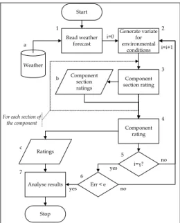
In this section a description of the algorithm responsible for the state estimation is given. The primary aim of the thermal state estimation algorithm is to allow the rating of components, which are not directly monitored within the power system, to be assessed. Thermal state estimations facilitate the precise and reliable assessment of environmental conditions whereby a minimal amount of meteorological monitoring installations facilitate the assessment of component thermal ratings within a wide area. This may then be validated through the carefully selected monitoring of component operating temperatures. The algorithm provides a reliable estimation of power system component thermal ratings described by an appropriate cumulative probability function. A state estimation technique based on the Montecarlo method is used, giving a more complete description of the possible states of the system. The minimum, maximum, average and standard deviation of component rating forecasts may be calculated according to the possible forecasted weather conditions. As necessary for overhead lines and electric cables, each component is divided into sections to take into account different thermal operating conditions such as overhead line orientations and changes in electric cable installation conditions. The section resulting in the lowest rating values is then used to provide a rating for the entire component. Furthermore, the deployment of a real-time thermal rating system underpinned by thermal state estimation techniques has the potential to reduce the necessity of auxiliary communications infrastructure whilst simultaneously increasing the reliability of the system if measurement or communication failures occur.

Start Read weather forecast Weather Generate variate for environmental conditions Component section rating Component rating i=0 i=γ? Err < e yes no yes no Analyse results Stop i=i+1 1 2 3 4 5 6 7 Ratings Component section ratings a b

For each section of the component

c

Fig. 2 Component rating estimation flow chart

The thermal state estimation algorithm is illustrated in Fig. 2, where it is possible to see the following steps:

1. Forecasted weather data is read from an external source (in this case the database “a”), where real-time readings from different meteorological station locations within the distribution network are stored.

2. A set of values for weather parameters is calculated in the following way: From the data read in “1” the parameters of a cumulative probability function are calculated. In this case the Beta probability function is used. A random value for the probability is selected and from the cumulative probability function the corresponding parameter value is found. This is repeated for each weather parameter.

3. For each section of the component the values of local environmental condition are calculated with the methodology described in Section 5.1, then the rating is calculated using the models described in Section 4. The result is stored temporarily in “b”.

4. The component rating is calculated by selecting the minimum rating of each section. The results are temporarily stored in “c”.

5. The steps from 2 to 4 are repeated for a fixed number of times γ.

6. The precision of the result is compared with a predefined value. If the result is not acceptable, a new value for γ is calculated and the steps from 2 to 5 are repeated

7. Component ratings stored in “c” are analysed in order to calculate the minimum, maximum, average value and standard deviation for each component of the network.

6. Generator output control strategies

This section describes strategies for the power output control of single and multiple generation installations.

6.1 Single generation installations

A number of different solutions are presented (ENA, 2003) that may be developed to manage, in an active manner, the power flows associated with the connection of a single generation installation. The most basic systems involve the disconnection of generation in the event that network power flow congestion occurs when utilising component static thermal ratings. This solution may be developed further by actively switching between seasonal ratings based on fixed meteorological assumptions and adjusting the number of disconnected generation units accordingly. More sophisticated solutions are developed from the principle of generator power output control, utilising technologies such as the pitch control of wind turbine blades to capture a desired amount of wind energy. In this approach the powers flowing in the critical feeders of the network are monitored, taking load demand into account, and the power exported from the generator is controlled to ensure the capability of the network is not exceeded. This may be developed as a solution utilising component static ratings, with demand-following control of the generator output, or as a solution utilising component real-time thermal ratings, with demand-following control of the generator output. Although generators may, at times, be requested to operate in voltage control mode, it is in the interest of the operators to maximise annual exported active energy (MWh) as that directly relates to the revenue of the generation installation owner. Thus it is assumed that the control system outlined in this chapter is utilised for generators exporting real power at unity power factor. An assessment of the real power output adjustment required by a generator may be calculated in Eq.37-38, relating to the component power flow sensitivity factor and the real-time thermal rating of the component



i,k P,m



k , i m , P dG dP P G    (37)



  

   

      _        _{ }  P_i,k U_Tar S_lim2 ''Q_i,k 2 'S_i,k 2 'Q_i,k 2 (38) where ΔGP,m (MW) is the required change in real power output of the generator at node m, ΔPi,k (MW) is the required change in real power flow through the component, from node i to node k in order to bring the resultant power flow back within thermal limits, dPi,k/dGP,m is the power flow sensitivity factor that relates the change in nodal real power injection at m with the change in real power flow seen in the component from node i to node k, ‟Si,k (MVA) is the apparent power flow in the component before control actions are implemented, ‟Qi,k (MVAr) is the reactive power flow in the component from node i to node k before the control actions are implemented, UTar is the target utilisation limit of the component after the control actions have been implemented, Slim (MVA) is the static or real-time thermal rating of the component and “Qi,k (MVAr) is the reactive power flow in the component from node i to node k after the control actions have been implemented. Rather than neglecting MVAr flow, it may be assumed constant for a particular operating condition. Thus dPi,k/dGP,m >> dQi,k/dGP,m and a simplification can be made to Eq.38 that “Qi,k ≈ ‟Qi,k.

6.2 Multiple generation installations

Present last-in first-off control strategies include the complete disconnection of generation installations or the power output reduction of generators in discrete intervals (Roberts, 2004). A step beyond this could be to implement a last-in first-off ‟sensitivity-based‟ control strategy whereby

generator power outputs are adjusted (in contractual order) based on Eq.37-38. Moreover, these equations may be developed further to define the power output adjustment of multiple generation installations (assuming contracts are in place to allow generator operation outside of a last-in first-off constraint priority) in order to maximise the annual energy yield of the aggregated generation installations. Two candidate strategies are outlined below:

1. Equal percentage reduction of generator power output

The equal percentage reduction signal, Φ, broadcast to multiple generators in order to proportionally reduce their power output (taking power flow sensitivity factors into account) may be assessed as in Eq.39-40.    G_P,m G_P,m (39)









     _  m 0 m P,m ik P,m ik dG dP G P (40)

This strategy may be seen as the most „fair‟ option since each generator is constrained as an equal proportion of their present power output.

2. Most appropriate technical strategy

In order to minimise the overall generator constraint and thus maximise the annual energy yield of the aggregated generators, an assessment of the required generator power output adjustment is given in Eq.41. In this case, rather than adjusting generators in contractual order according to the historical order of connection agreements, the generator constraint order is prioritised according to the magnitude of the power flow sensitivity factors. Thus the generator with the greatest technical ability to solve the power flow congestion is adjusted first.





max m , P k , i ik min m , P _{{dP dG}P _} G    (41)

7. Case study: Power output control of multiple

generators informed by component thermal

ratings

The following case study illustrates various aspects of the development of a power output control system for generation installations. An assessment of power flow sensitivity factors is made which allows thermal vulnerability factors to be calculated. This informs the development of a real-time thermal rating algorithm for an electric cable section within the case study network. An offline simulation is conducted which allows the energy yield of candidate strategies for the power output control of multiple generators (informed by static and real-time thermal ratings) to be assessed.

7.1 Case study network description

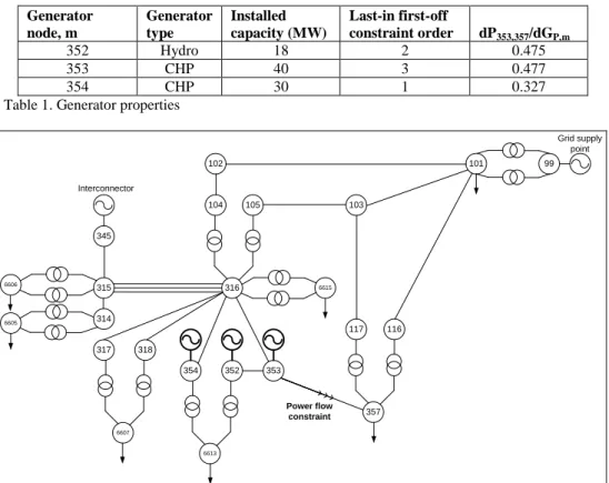
The case study network shown in Fig. 3 was derived from a section of the United Kingdom generic distribution system (UKGDS) „EHV3‟ network (Foote et al., 2006). A hydro generator and two combined heat and power (CHP) generators were connected to the network at 33kV nodes. A summary of the generator properties is given in Table 1.

Generator node, m Generator type Installed capacity (MW) Last-in first-off constraint order dP353,357/dGP,m 352 Hydro 18 2 0.475 353 CHP 40 3 0.477 354 CHP 30 1 0.327

Table 1. Generator properties

99 101 102 104 105 103 316 6615 117 116 357 353 352 354 6613 318 317 6607 315 314 6606 6605 345 Grid supply point Power flow constraint Interconnector

Fig. 3 United Kingdom generic distribution system case study

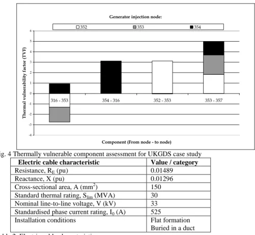
7.2 Thermal vulnerability factor assessment

The most thermally vulnerable components within the case study network were identified using a thermal vulnerability factor assessment as given in Fig. 4 (and detailed in Sections 3.1 and 3.2). From this assessment it may be seen that a generator real power injection at node 352 increases the thermal vulnerability of the components between nodes 352 and 353, and between nodes 353 and 357 but reduces the thermal vulnerability of the component between nodes 316 and 353. Moreover, a generator real power injection at node 353 increases the thermal vulnerability of the component between nodes 353 and 357 but reduces the thermal vulnerability of the component between nodes 316 and 353. Furthermore, a generator real power injection at node 354 increases the thermal vulnerability of the components between nodes 316 and 353, 354 and 316, and 353 and 357. However, this injection has little impact on the thermal vulnerability of the component between nodes 352 and 353. In this particular case, multiple generator injections cause the thermal vulnerability

factors to accumulate for the electric cable between nodes 353 and 357, making it the most thermally vulnerable component. Having identified this component as being a potential thermal pinch-point and causing power flow congestion within the network, the targeted development of a real-time thermal rating system is informed.

7.3 Component real-time thermal rating assessment

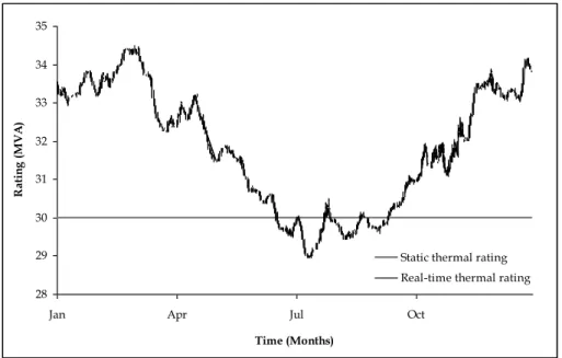
A summary of the characteristics of the thermally vulnerable electric cable are given in Table 2. The ‟Valley‟ UK MetOffice dataset for the calendar year 2006 was used with the thermal state estimation technique described by Eq.31-36 (Section 5.1) to estimate environmental operating conditions local to the electric cable. This information was used to populate the electric cable steady-state thermal model described by Eq.26 (Section 4.2). The resulting real-time thermal rating for the electric cable, together with the static rating, is given in Fig. 5. It was found that the average uprating for the electric cable, based on minimum daily ratings was 6.0% across the year.

Generator injection node:

-4 -3 -2 -1 0 1 2 3 4 5 6 316 - 353 354 - 316 352 - 353 353 - 357

Component (From node - to node)

T h er m al v u ln er ab il it y fac to r (T VF ) 352 353 354

Fig. 4 Thermally vulnerable component assessment for UKGDS case study Electric cable characteristic Value / category

Resistance, RE (pu) 0.01489

Reactance, X (pu) 0.01296

Cross-sectional area, A (mm2) 150 Standard thermal rating, Slim (MVA) 30 Nominal line-to-line voltage, V (kV) 33 Standardised phase current rating, I0 (A) 525

Installation conditions Flat formation

Buried in a duct Table 2. Electric cable characteristics

7.5 Electro-thermal simulation approach

This section describes the offline electro-thermal simulation that was used to quantify the individual and aggregated generator annual energy yields (as seen in Section 7.6) for the candidate multiple generator control strategies. UKGDS annual ½ hour loading and generation profiles were utilised for the simulation of network power flows and busbar voltages through a load flow software tool. The open-loop power output control system compared network power flows to component static and real-time thermal limits for each ½ hour interval within the simulated year. When power flow congestion was detected (signified in this case by an electric cable utilisation, U353,357 > 1) the controller implemented the relevant generator power output control algorithm as described below. A validating load flow simulation was conducted as part of the control solution to ensure that the updated generator power outputs solved the power flow congestion and did not breach busbar voltage limits (set to ±6% of nominal). 28 29 30 31 32 33 34 35

Jan Apr Jul Oct

Time (Months) R atin g (MV A )

Static thermal rating Real-time thermal rating

Fig. 5 Electric cable static and real-time thermal rating

The individual and aggregated generator power outputs were integrated across the simulated year in order to calculate the potential annual energy yields resulting from the candidate multiple generator control strategies, informed by component static and real-time thermal limits. The results are summarised in Section 7.6.

1. Last-in first-off discrete interval generator output reduction

In order to solve the power flow congestion, the power output of the generators was reduced in discrete intervals of 33% according to the contractual priority order given in Table 1. Thus the power output of the generator at node 354 was reduced by 33% then 66% followed by generator disconnection and the 33% power output reduction of the generator at node 352.

Using Eq.38 with UTar = 0.99, the required real power reduction in the electric cable, ΔP353,357 in order to bring the resultant power flow back within the desired thermal limit was calculated. The required reduction in the power output of the first generator (contractually) to be constrained, ΔGP,354, was calculated using Eq.42 for GP,354 – ΔGP,354>0 and the output from GP,353 and GP,352 was unconstrained. On occasions when the required constraint of the generator at node 354 would result in GP,354 – ΔGP,354<0, the generator was disconnected and the remaining power flow congestion was solved by the next generator (at node 352) to be contractually constrained.

327 . 0 P Gp,354 353,357    (42)

3. Equal percentage reduction of generator power outputs

Using Eq.38 with UTar = 0.99, the required real power reduction in the electric cable, ΔP353,357 in order to bring the resultant power flow back within the desired thermal limit was calculated. The equal percentage reduction signal, Φ, broadcast to all generators in order to solve the power flow congestion was calculated and implemented using Eq.43-46.

354 , p 352 , p 353 , p 357 , 353 G 327 . 0 G 475 . 0 G 477 . 0 P      (43)    G_p,353 G_p,353 (44)    G_p,352 G_p,352 (45)    G_p,354 G_p,354 (46)

4. Most appropriate technical strategy

Using Eq.38 with UTar = 0.99, the required real power reduction in the electric cable, ΔP353,357 in order to bring the resultant power flow back within the desired thermal limit was calculated. Since, in this case, Gp,353 has the greatest technical ability to solve power flow congestion (as assessed by the comparative magnitude of power flow sensitivity factors in Table 1), Eq.47 was implemented to minimise the overall generation constraint and thus maximise the annual energy yield of the aggregated generators. On occasions when the required constraint of the generator at node 353 would result in GP,353 – ΔGP,353<0, the generator was disconnected and the remaining power flow congestion was solved by the generator with the next-greatest power flow sensitivity factor (in this case at node 352). 477 . 0 P Gp,353 353,357    (47)

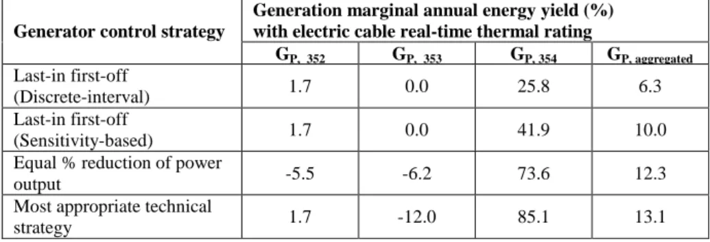
7.6 Findings

The marginal annual energy yields resulting from the applied candidate control strategies informed by the electric cable real-time thermal ratings are summarised in Table 3. A similar table is given (Jupe & Taylor, 2009a) for the marginal energy yields resulting from static component ratings. The last-in first-off ‟discrete interval‟ strategy with static component ratings was used as a datum with annual energy yields of 106.38GWh, 298.26GWh, 120.84 GWh and 525.48GWh for GP, 352, GP, 353, GP, 354 and GP, aggregated respectively.

Generator control strategy

Generation marginal annual energy yield (%) with electric cable real-time thermal rating

GP, 352 GP, 353 GP, 354 GP, aggregated

Last-in first-off

(Discrete-interval) 1.7 0.0 25.8 6.3

Last-in first-off

(Sensitivity-based) 1.7 0.0 41.9 10.0

Equal % reduction of power

output -5.5 -6.2 73.6 12.3

Most appropriate technical

strategy 1.7 -12.0 85.1 13.1

Table 3. Generation marginal annual energy yields

8. Discussion

Considering Table 3, for the case study network it can be seen that the adoption of both real-time thermal rating systems and sensitivity factor-based generator power output control strategies have the potential to unlock gains in the aggregated annual energy yield contribution of multiple generation installations. Moving from a static rating system to a real-time rating system has the potential to unlock an extra 6.3% aggregated annual energy yield for the last-in first-off ‟discrete interval‟ power output reduction strategy. If a last-in first-off contractual priority is retained but a sensitivity-based power output control strategy is adopted this has the potential to unlock an extra 3.7% marginal aggregated annual energy yield. Moreover, a further 3.1% annual energy yield gain may be achieved by utilising the „most appropriate technical‟ strategy that minimises overall generator constraint. For the „equal percentage reduction of generator power output‟ strategy, it can be seen that the relative annual energy yields of GP,352 and GP,353 are reduced in order to achieve an aggregated generator annual energy yield gain. This phenomenon is even more pronounced in the „most appropriate technical‟ strategy where annual energy yield gains of 1.7% and 85.1% for GP,352 and GP,354 respectively are facilitated by the 12.0% reduction in the annual energy yield of GP,353.

The aim of this research was to outline the developmental stages required in the output control of generation installations for improved new and renewable energy yield penetrations. The purpose of the thermal vulnerability factor assessment was to identify thermally vulnerable components within distribution networks. It has been shown that the thermal vulnerability factor assessment is appropriate for use in a strategic way to assess longer term and wide-spread generation growth scenarios. Therefore the thermal vulnerability factor assessment procedure would be valuable for DNOs looking to develop long-term generation accommodation strategies for areas of their network. Furthermore, the thermal vulnerability factor assessment identifies those components that would most benefit from being thermally monitored to unlock latent power flow capacity through a real-time

thermal rating system. The derived power flow sensitivity factors are network configuration-specific and assume that the network configuration will not be frequently changing. It is feasible, however, to develop an online control system that makes use of alternative sets of the above mentioned predetermined power flow sensitivity factors based on network switch status information. In order to deploy the control strategies presented there clearly needs to be a contractual mechanism in place that gives an incentive to separately owned generators to have their power output reduced in order to maximise the overall annual energy yield. One such mechanism could be to set up cross-payments between generators whereby the generators that are constrained to maximise the aggregated energy yield are rewarded by payments from the other generators.

9. Conclusion

It is anticipated that distribution networks will continue to see a proliferation of generation from new and RE resources in coming years. In some cases this will result in power flow congestion with thermally vulnerable components restricting the installed capacity and energy yield penetration of generators. Therefore a system that can be developed for the management of power flows within distribution networks, through the power output control of generators, could be of great benefit. The development stages of such a system were outlined in Sections 3 – 6. These included: (i) the identification of thermally vulnerable components through a thermal vulnerability factor assessment that related power flow sensitivity factors to component thermal limits, (ii) the targeted development of thermal models to allow latent capacity in the network assets to be unlocked through a real-time thermal rating system, (iii) the development of thermal state estimation techniques that would allow component steady-state thermal models to be populated with real-time data from meteorological monitoring equipment installed in the distribution network (iv) the use of the real-time thermal ratings together with power flow sensitivity factors to control the power output of multiple generators. The development stages were illustrated with a case study and the energy yields resulting from the offline application of strategies were quantified. It was demonstrated for the particular case study scenario that the adoption of both a real-time thermal rating system and power flow sensitivity factor-based control strategies have the potential to unlock gains in the aggregated annual energy yield of multiple generation installations. Work is continuing in this area to realise the potential of generator output control systems for increased new and renewable energy yield penetrations.

10. References

Abu-Hamdeh, N.H. (2003). Thermal properties of soil as affected by density and water content.

Biosystems engineering, Vol. 86, No.1 (September 2003) 97-102

ANSI/IEEE. (1981). C57.92 Guide for loading mineral oil-immersed power transformers up to and

including 100 MVA with 55°C or 65°C average winding rise, IEEE

Belben, P.D. & Ziesler, C.D. (2002). Aeolian uprating: how wind farms can solve their own transmission problems, Proceedings of 1st World Wind Energy Conference and Exhibition,

Berlin, Germany, July 2002

Berende, M.J.C., Slootweg, J.G. & Clemens, G.J.M.B. (2005). Incorporating Weather Statistics in Determining Overhead Line Ampacity, Proceedings of International Conference on Future

Power Systems, 1-8, ISSN 90-7805-02-4, Amsterdam, Netherlands, November 2005, FPS,

Celia, M.; Boulotas, E. & Zarba, R. (1990). A general mass-conservative numerical solution for the unsaturated flow problem. Water resources research, Vol. 26, No.7, 1483-1496

Currie, R. A. F.; Ault, G. W. & McDonald, J. R. (2006). Methodology for determination of economic connection capacity for renewable generator connections to distribution networks optimised by active power flow management. IEE Generation, Transmission, Distribution, Vol. 153, No. 4, (July 2006), 456-462, ISSN 1350-2360

Dinic, N.; Flynn, D.; Xu, L. & Kennedy, A. (2006). Increasing Wind Farm Capacity. IEE Generation,

Transmission, Distribution, Vol. 153, No. 4, (July 2006), 493-498, 1350-2360

Douglass, D. A. & Edris A. A. (1996). Real-time monitoring and dynamic thermal rating of power transmission circuits. IEEE Transactions on Power Delivery, Vol. 11, No. 3, (July 1996), 1407-1418, ISSN 0885-8977

Douglass D. A.; Edris A. A. & Pritchard G. A. (1997). Field application of a dynamic thermal circuit rating method. IEEE Transactions on Power Delivery, Vol. 12, No. 2, (April 1997), 823-831, ISSN 0885-8977

Electricity Networks Association. (1971). Engineering Recommendation P15: Transformers loading

guide, ENA, London

Electricity Networks Association. (1986). Engineering Recommendation P27: Current rating guide

for high voltage overhead lines operating in the UK distribution system, ENA, London

Electricity Networks Association. (2003). Engineering Technical Report 124: Guidelines for actively

managing power flows associated with the connection of a single distributed generation plant, ENA, London

Electricity Networks Association. (2004). Engineering Recommendation P17: Current rating for

distribution cables, ENA, London

Foote, C.; Djapic, P.; Ault, G.; Mutale, J.; Burt G. & Strbac, G. (2006). United Kingdom Generic

Distribution System (UKGDS) - Summary of EHV Networks, DTI Centre for Distributed

Generation and Sustainable Electrical Energy, UK

Fox-Penner, P.S. (2001). Easing Gridlock on the Grid - Electricity Planning and Siting Compacts. The

Electricity Journal, Vol. 14, No.9 (November 2001), 11-30

Harrison, G.P. & Wallace, A.R. (2005). Optimal Power Flow Evaluation of Distribution Network Capacity for the Connection of Distributed Generation. IEE Generation, Transmission,

Distribution, Vol. 152, No. 1, (January 2005), 115-122, ISSN 1350-2360

Helmer, M. (2000). Optimized size of wind power plant transformer and parallel operation,

Proceedings of Wind Power for the 21st century, Kassel, Germany, September 2000

Hoffmann, S.P. & Clark, A.M. (2004). The approach to thermal uprating of transmission lines in the UK. Electra, (B2-317), CIGRE, Paris

House, H.E. & Tuttle, P. D. (1959). Current Carrying Capacity of ACSR. IEEE Transactions on

Power Apparatus Systems, Vol. 78, No. 3, (April 1958), 1169-1177, ISSN 0018-9510

IEC. (1991). IEC 60826: Loading and strength of overhead transmission lines, IEC, Switzerland IEC. (1994). IEC 60287: Electric cables – calculation of the current rating, IEC, Switzerland IEC. (1995). IEC TR 1597: Overhead electrical conductors – calculation methods for stranded bare

conductors, IEC, Switzerland

IEC. (2008). IEC 60076-7: Power transformers - Part 7: Loading guide for oil-immersed power

transformers, IEC, Switzerland

IEEE. (1993). IEEE 738: Standard for calculating the current-temperature relationship of bare

overhead conductors, IEEE

IEEE. (1994). IEEE 835, IEEE Standard Power Cable Ampacity Tables, IEEE

Ippolito, L., Vaccaro, A., Villacci, D. (2004). The use of affine arithmetic for thermal state estimation of substation distribution transformers. International Journal for Computation and

Mathematics in Electrical and Electronic Engineering, Vol. 23, No. 1, 237–249, ISSN