RESEARCH ARTICLE
Age-based partitioning of individual
genomic inbreeding levels in Belgian Blue cattle
Marina Solé
1*, Ann‑Stephan Gori
1,2, Pierre Faux
1, Amandine Bertrand
1, Frédéric Farnir
3, Mathieu Gautier
4,5and Tom Druet
1Abstract
Background: Inbreeding coefficients can be estimated either from pedigree data or from genomic data, and with genomic data, they are either global or local (when the linkage map is used). Recently, we developed a new hid‑ den Markov model (HMM) that estimates probabilities of homozygosity‑by‑descent (HBD) at each marker position and automatically partitions autozygosity in multiple age‑related classes (based on the length of HBD segments). Our objectives were to: (1) characterize inbreeding with our model in an intensively selected population such as the Belgian Blue Beef (BBB) cattle breed; (2) compare the properties of the model at different marker densities; and (3) compare our model with other methods.
Results: When using 600 K single nucleotide polymorphisms (SNPs), the inbreeding coefficient (probability of sampling an HBD locus in an individual) was on average 0.303 (ranging from 0.258 to 0.375). HBD‑classes associated to historical ancestors (with small segments ≤ 200 kb) accounted for 21.6% of the genome length (71.4% of the total length of the genome in HBD segments), whereas classes associated to more recent ancestors accounted for only 22.6% of the total length of the genome in HBD segments. However, these recent classes presented more individual variation than more ancient classes. Although inbreeding coefficients obtained with low SNP densities (7 and 32 K) were much lower (0.060 and 0.093), they were highly correlated with those obtained at higher density (r = 0.934 and 0.975, respectively), indicating that they captured most of the individual variation. At higher SNP density, smaller HBD segments are identified and, thus, more past generations can be explored. We observed very high correla‑ tions between our estimates and those based on homozygosity (r = 0.95) or on runs‑of‑homozygosity (r = 0.95). As expected, pedigree‑based estimates were mainly correlated with recent HBD‑classes (r = 0.56).
Conclusions: Although we observed high levels of autozygosity associated with small HBD segments in BBB cattle, recent inbreeding accounted for most of the individual variation. Recent autozygosity can be captured efficiently with low‑density SNP arrays and relatively simple models (e.g., two HBD classes). The HMM framework provides local HBD probabilities that are still useful at lower SNP densities.
© The Author(s) 2017. This article is distributed under the terms of the Creative Commons Attribution 4.0 International License (http://creativecommons.org/licenses/by/4.0/), which permits unrestricted use, distribution, and reproduction in any medium, provided you give appropriate credit to the original author(s) and the source, provide a link to the Creative Commons license, and indicate if changes were made. The Creative Commons Public Domain Dedication waiver (http://creativecommons.org/ publicdomain/zero/1.0/) applies to the data made available in this article, unless otherwise stated.
Background
Two alleles are identical-by-descent (IBD) if they descend from a single allele in an ancestor. This measure is rela-tive and depends on the definition of a reference (or base) population. Indeed, two alleles are declared IBD if the ancestor belongs to the reference population and iden-tical-by-state (IBS) for more remote common ancestors.
When two alleles are IBD within an individual, the terms “autozygous” or “homozygous-by-descent” (HBD) are used. The inbreeding coefficient F of an individual is related to these measures and is defined as the probability
that two alleles at any locus in this individual are IBD [1].
Inbreeding is associated with negative effects on fitness
(e.g., [2–4]) and the occurrence of monogenic disorders
increases in populations with higher levels of
inbreed-ing [5]. Thus, the study and management of inbreeding
are of high importance in such populations. Belgian Blue Beef cattle (BBB) represent a good example of an inten-sively selected cattle population. A consequence of the
Open Access
*Correspondence: [email protected]
1 Unit of Animal Genomics, GIGA‑R & Faculty of Veterinary Medicine, University of Liège, B34 (+1) Avenue de l’Hôpital 1, 4000 Liège, Belgium Full list of author information is available at the end of the article
selection process in this breed is the increase in the level of inbreeding, as illustrated by several recent outbreaks
of genetic recessive defects [5–11].
There are several methods to estimate the inbreed-ing coefficient F. In the past, methods were based on the genealogy and estimated the expected inbreeding coef-ficient (based on the relationship between the two par-ents). With the development of genetic markers, several approaches allow the estimation of the realized inbreed-ing coefficient (“observed” in an individual), even in the absence of genealogy. Global approaches, including
moments estimators (e.g., [12]), simple homozygosity
measures (e.g., [2]) or based on the genomic
relation-ship matrix [13], estimate the total amount of inbreeding
in an individual and can work with sparse genetic maps. Methods that are based on runs of homozygosity (ROH)
(e.g., [14]) are, most often, empirical rule-based methods,
which assume that long stretches of identical alleles are HBD. For such rule-based methods, prior parameters have to be defined, i.e., the minimal number of homozy-gous markers, the minimal length and the maximum number of allowed heterozygous markers to consider a set of successive markers as HBD, etc. Likelihood-based
approaches (e.g., [15, 16]) rely on probabilistic models,
which use allele frequencies and genotyping error rates to determine whether ROH are autozygous (i.e., HBD), and derive from earlier works by Broman and Weber
[17]. Compared to global estimators, ROH-based
meth-ods require denser genetic maps and can provide estima-tors of local autozygosity. ROH have been used to study
inbreeding in diverse species including humans [14, 16,
18], pigs [19], cattle [20, 21] and others, and to study
genetic diversity and signatures of selection. In addi-tion, ROH offer the possibility to distinguish between
recent and more ancient inbreeding [16, 18, 22]. Indeed,
segments that are inherited from recent ancestors are expected to be longer since the recombination process has fewer generations to split the fragment into smaller pieces. Finally, hidden Markov models (HMM) were developed to estimate the HBD probability of segments
along chromosomes [23] and make use of all the
avail-able information about the sequences of homozygous/ heterozygous markers, allele frequencies of markers, the genetic map, and genotyping error rates. These models
can handle whole-genome sequence data [24],
includ-ing low-fold experiments [25]. All these HMM assume
that (1) all the autozygosity results from a single event, (2) all the HBD segments trace back to one or several ancestors in a single generation, and (3) they all have the same expected length. However, natural and domesti-cated populations are complex. They result from a long demographic history with variable effective population
size (Ne) and, sometimes, have undergone major demo-graphic events such as bottlenecks.
To relax this strong assumption of the current HMM methods, we recently developed a new HMM with
mul-tiple age-based HBD-classes [26] in which the length of
the HBD segments from different classes have distinct expected distributions (longer/shorter segments for more recent/ancient common ancestors). The model allows to fit genomic data better and to reveal the “recent” demo-graphic history of populations. The aims of our study were to: (1) characterize inbreeding by using a model describing genomes as a mosaic of non-HBD and HBD segments and partitioning the latter in multiple age-related classes in an intensively selected cattle population such as BBB cattle; (2) investigate the effect of marker density and setting of parameters on the estimates; and (3) compare our estimates with those obtained with other methods (pedigree-based inbreeding coefficients, estimates from the genomic relationship matrix or rule-based ROH estimators).
Methods Data
Single nucleotide polymorphism (SNP) genotypes for the 735,293 SNPs from the Illumina BovineHD Bead-Chip (HD; Illumina, San Diego, CA) were available for 634 BBB sires. Moreover, whole-genome sequencing (WGS) data were also available for 50 of these sires (the bioinformatic processing of the WGS data is described
in [27]). The pedigree including all known ancestors of
the 634 bulls contained 7676 individuals. In addition,
we extracted from the Widde database (http://widde.
toulouse.inra.fr; [28]), Illumina BovineHD genotypes for animals belonging to 10 cattle breeds of European origin (originally provided by the BovineHD genotyping con-sortium). This set contained samples from 42 Angus, 22 Brown Swiss, 37 Charolais, 21 Guernsey, 35 Hereford, 60 Holstein, 38 Jersey, 50 Limousin, 21 Piedmontese and 21 Romagnola individuals.
All individuals had a call rate higher than 0.90. We selected SNPs that mapped to bovine autosomes (using the UMD3.1 build) and removed from the dataset those that had a call rate lower than 95% and minor allelic fre-quency lower than 0.01, that significantly deviated from Hardy–Weinberg proportions (p < 0.001) or that pre-sented incompatible genotypes for more than one par-ent–offspring pair, which resulted in a set of 601,226 SNPs. Furthermore, SNPs located in segments that might be incorrectly mapped to the genome build were removed. Such putative errors were identified based on
evidence from linkage information [29], linkage
independent samples [31]. Consequently, an additional 2.7% of the SNPs were filtered out, which resulted in a final BBB dataset of 585,159 SNPs. Removing potential map errors is essential for our applications since these might break long ROH into smaller fragments. For the other breeds, the number of conserved SNPs using the same rules ranged from 524,113 to 622,603 SNPs.
To study the effect of SNP density on the estima-tion of inbreeding, we used two subsets of the 585,159 SNPs selected for BBB cattle based on their presence on the bovine Illumina BovineSNP50 BeadChip v1 and v2 (32,412 SNPs conserved for this 50 K panel) or on both the 50 K panel and the Illumina BovineLD BeadChip (6844 SNPs conserved for this low-density (LD) panel).
For the sequence data, first we applied stringent fil-tering rules to select a high-quality subset of SNPs, as
described in [31]. Briefly, SNPs, which passed the
calibra-tion score and were present in other cattle WGS
data-sets (1000 bull genomes project [32], Holstein and Jersey
individuals from New-Zealand [27] and a Dutch Holstein
pedigree of 415 individuals that was used as a reference
population for imputation in [33]), were selected,
result-ing in a set of ancient variants. We conserved only the SNPs that presented correct Mendelian segregation in
the WGS Dutch Holstein pedigree (see [33] for more
details). Regarding the genotyping data, we also removed variants with a MAF lower than 0.01 and some possibly incorrectly mapped regions (errors in the genome
assem-bly) based on the rules described in [31]. The final WGS
dataset contained 5,653,911 bi-allelic SNPs.
Methods to estimate inbreeding coefficients and HBD probabilities
Multiple HBD‑classes HMM
Our multiple HBD-classes model [26] is a HMM that
describes individual genomes as mosaics of multiple HBD and non-HBD states. Although several non-HBD states can be fitted, here we used only one non-HBD state and K − 1 HBD states for a total of K states, where K is a parameter of the method that can be either predefined or selected by model comparison (see below). Each state k has its own rate parameter Rk that defines the
distribu-tion of the lengths of the segments originating from that class: the lengths in Morgans are distributed
exponen-tially with rate Rk. The rate corresponds approximately
to the size of the inbreeding loop measured in genera-tions and is closely related to age in generagenera-tions of the
common ancestors. Rk is approximately twice the
num-ber of generations to the common ancestor. Each state has also its own mixing proportion, which is equal to the frequency of segments originating from that class. Such a model with multiple-HBD classes will be referred to as a KR model, with K being equal to the number of
distinct rates fitted, K − 1 for HBD states and 1 for the non-HBD state. In the case where a single HBD class and a single non-HBD class are fitted, we use a common rate for both (1R model) since such a model has better
properties [26]. Emission probabilities of the HMM
cor-respond to the probabilities of observing a particular genotype conditionally on the underlying state (HBD or non-HBD). For non-HBD classes, these probabilities
correspond to Hardy–Weinberg proportions [26] and
for HBD classes, homozygotes AA are observed with a
probability fA (1 − ε ) and heterozygotes with a probability
ε , where f
A is the frequency of allele A and ε is an error
term corresponding to the probability of observing a
het-erozygous genotype in a HBD segment [26]. With WGS
data, these probabilities are integrated over the different
genotype probabilities obtained from the VCF file [26].
For each HBD class, the genome-wide HBD probability is estimated as the probability of belonging to that class averaged over the whole genome, whereas the local HBD probability is defined as the probability of belonging
to that class at a specific genomic location (see [26] for
more details). The genome-wide HBD probabilities cor-respond to the percentage of the genome that is associ-ated with a specific HBD class, e.g., the proportion of the genome that is located within HBD segments of a certain length. To estimate the inbreeding coefficient, first the base population must be defined, which is done by decid-ing which classes are considered as truly autozygous. For instance, we might consider that ancestors associated
with classes with a Rk rate higher than a selected
thresh-old T (i.e., Rk ≥ T) are unrelated. Then, the corresponding
inbreeding coefficient FG-T is estimated as the probability
to belong to any of the HBD classes with a Rk ≤ T
aver-aged over the whole genome (e.g., the inbreeding coef-ficient is defined as the probability of sampling an HBD
locus given a reference population). Since Rk rates of
HBD classes are approximately equal to twice the num-ber of generations to the common ancestor, including
HBD classes with a Rk ≤ T amounts to setting the base
population to approximately 0.5 * T generations ago. In the remainder of the manuscript, inbreeding coefficients or HBD probabilities reported without specifying a base
population or Rk, are obtained by including all HBD
classes (e.g., using the most remote base population). In that case, the age of the base population or the smallest HBD segments captured are a function of the SNP den-sity used. All the HBD probabilities are estimated with
the forward–backward algorithm [34].
As an alternative to the KR model, we can use a set of
pre-defined Rk rates and estimate only the mixing
pro-portions (MixKR model). This set of Rk rates should be
selected to cover a wide range of past generations. In our
equal to [21, 22, 23, …, 213] and one non-HBD class with a
rate of 213. These values were chosen to have a constant
and limited degree of overlap between the exponential distributions that specify the HBD lengths for each suc-cessive class. The upper rate is determined by the SNP density that defines the size of the smallest HBD seg-ments that we can capture. Such models proved efficient to estimate the genome-wide (global) and local autozy-gosity levels and to obtain information on recent
demo-graphic history [26]. In addition, inbreeding coefficients
are then estimated with respect to the same reference population and HBD classes are defined over identical periods in the past, allowing better comparisons between individuals.
With all the models, the parameters (mixing
propor-tions for all models and Rk rates for KR models only)
were estimated with 1000 iterations of the
expectation-maximization algorithm with constraints to force Rk to
be between 1 and 8192. The number of classes K is fixed for each run but the optimal value can be determined by comparing models with the Bayesian information criterion (BIC). All analyses were performed with the
ZooRoH software (https://github.com/tdruet/ZooRoH).
Additional inbreeding coefficient estimators
The inbreeding coefficient based on pedigree data (FPED)
was computed with the method of Sargolzaei et al. [35].
We used several measures to estimate genomic inbreed-ing coefficients. The first measure uses the diagonal elements of the genomic relationship matrix (GRM)
computed with the BLUPF90 package [36] without any
pedigree information (α set to 1.0) and is based on the
variance of the additive genetic values (FGRM; [13, 37]).
The second, which was proposed and recommended
by Yang et al. [38] for its smaller sampling variance, is
based on the correlation between uniting gametes (FUNI)
and was estimated using the GCTA software [39]. The
third more simple measure is defined as the
homozygo-sity (FHOM) or the proportion of homozygous SNPs (e.g.,
[2]), which is closely related to the excess homozygosity
estimator (FExHOM) implemented in plink [40]. For FGRM,
FUNI and FExHOM, we estimated allele frequencies based
on the 31 bulls born before 1985. Finally, the fourth esti-mator measures the proportion of the genome covered
by ROH (FROH), which contained at least 15 SNPs and
were identified using plink [40] with 50-SNP windows
(no heterozygous genotypes were accepted and up to five missing genotypes were possible). These parameters were
selected based on published studies in cattle (e.g., [20, 22,
41]). The minimal SNP density, length of ROH and
maxi-mal SNP spacing were optimized for each panel as fol-lows by order of increasing density: at least one SNP per 500, 100 and 10 kb, the length of ROH had to be at least
5 Mb, 1 Mb and 100 kb long and the maximum distance between two consecutive SNPs had to be 1 Mb, 500 kb and 200 kb.
Results
Estimation and age‑based partitioning of individual genomic inbreeding levels in the Belgian Blue Beef cattle population
We started by using a Mix14R model (with Rk ranging
from 2 to 8192) to estimate the proportion of the genome belonging to different HBD classes for the 634 BBB sires
(Fig. 1a), which allows the estimation of the inbreeding
coefficient with respect to different base populations as
explained in Methods (Fig. 1b). When considering all
HBD classes, the fraction of the genome that is HBD (corresponding to the inbreeding coefficient estimated with the most remote base population) was equal to 0.303 on average (ranging from 0.258 to 0.375), with a
major contribution from HBD-classes with high Rk rates
(Rk > 256) that account for 71.4% of the total HBD
pro-portion on average. These small ROH reflect the history of the population (background inbreeding and linkage disequilibrium associated with past effective population
size (Ne)) better than individual variation. Classes
asso-ciated with smaller Rk rates (i.e., with longer HBD
seg-ments) accounted for a smaller proportion of the total HBD proportion (the average inbreeding coefficient was equal to 0.054 and 0.087 when including HBD-classes
with Rk ≤ 32 and Rk ≤ 256, respectively, and setting the
base population approximately 16 or 128 generations ago) but presented more variation among individuals. For instance, the inbreeding coefficient associated with common ancestors tracing back up to approximately four generations ago (corresponding to HBD-classes
with Rk ≤ 8) ranged from 0.000 to 0.137. For bulls born
from 1980 to 2010, the percentage of the genome in HBD segments increased by 3.3% (+ 0.11% per year), i.e.,
approximately from 28 to 31% (see Additional file 1: Fig.
S1a). However, the trend for more recent HBD classes
(Rk ≤ 32) was more pronounced (see Additional file 1:
Fig. S1b), i.e., from almost 0 to 6% (+ 0.20% per year) and corresponded more closely to the trend observed with pedigree-based inbreeding coefficients (see Additional
file 1: Fig. S1c). Bulls born before 1980 presented little
evidence of recent autozygosity compared to modern bulls.
To assess the contribution of each HBD class to the percentage of the genome in HBD segments and to its variation in BBB cattle, we divided the total fraction of the genome in HBD classes [0.303 on average; standard deviation (SD) = 0.071] in four main classes (very recent
HBD classes with Rk = 2 to 8, recent HBD classes with
0.00 0.05 0.10 0.15 0.20 0.25
Percentage of the genome in HBD class
Rk =2 Rk =4 Rk =8 Rk =16 Rk =32 Rk =64 Rk =12 8 Rk =25 6 Rk =51 2 Rk =1024 Rk =2048 Rk =4096 Rk =8192
Rate of the HBD class a 0.00 0.05 0.10 0.15 0.20 0.25 0.30 0.35
Genomic inbreeding coefficient (F
G−
T
)
2 4 8 16 32 64 128 256 512 1024 2048 4096 8192
Value of the threshold T used to estimate FG−T (using HBD classes with RK≤ T) b
Fig. 1 Partitioning of genome‑wide autozygosity for the 634 Belgian Blue sires using the BovineHD SNP panel. a Boxplot of percentages of indi‑ vidual genomes associated with 13 HBD‑classes with pre‑defined Rk rates (Mix14R model). The percentages correspond to individual genome‑wide
probabilities of belonging to each of the HBD‑classes. b Genomic inbreeding coefficients estimated with respect to different base populations (FG‑T)
obtained by selecting different thresholds T that determine which HBD‑classes are considered in the estimation of FG‑T (e.g., setting the base popu‑
lation approximately 0.5 * T generations in the past). The corresponding inbreeding coefficients FG‑T are estimated as the probability of belonging to
and very ancient HBD classes with Rk = 1024 to 8192),
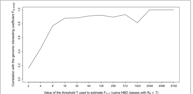
with each group having three HBD classes except the last one with four HBD classes. The average fraction of the genome associated with each of these main classes (ordered from recent to ancient) was equal to 0.027 (SD = 0.029), 0.041 (SD = 0.019), 0.054 (SD = 0.013) and 0.180 (SD = 0.011). Note that high proportions of very recent HBD segments are mechanically associated with lower proportions of very ancient HBD segments (r = − 0.407) because recent HBD segments mask more ancient HBD segments. Although the percentage of the genome in HBD classes associated with recent common ancestors represents only 22.6% of the total autozygosity, it displays more individual variation than that in more ancient classes (more than 50% of the total variance is associated with very recent HBD classes). By fitting a linear model, we estimated that very recent HBD classes account for 59% of the total autozygosity variation and that adding recent HBD classes to the model increases this value to 83%. Similarly, the correlations between inbreeding coefficients measured with respect to dif-ferent base populations (e.g., including difdif-ferent HBD classes in the computation) with the inbreeding coeffi-cients estimated using all HBD classes increased abruptly
from 0.16 for estimates based on the first class (Rk = 2)
to 0.77 for inbreeding coefficients estimated including
HBD classes with a Rk ≤ 8 and to 0.90 with a Rk ≤ 16, and
then improved only marginally by adding more
HBD-classes (Fig. 2). The decrease in correlation observed at
Rk = 1024 results from the fact that ancient autozygosity
is concentrated at Rk = 1024 for some individuals and at
Rk = 2048 for others.
Comparison of the results for BBB cattle with those of other breeds
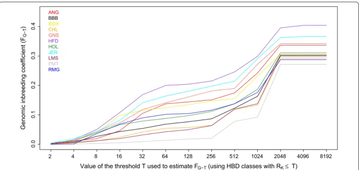
To determine whether comparable levels and patterns of autozygosity are also observed in other breeds of Euro-pean origin, we applied the same model to 10 breeds
genotyped with the same array (Fig. 3). In most of these
breeds, inbreeding coefficients estimated with respect to different base populations increased moderately up to FG-256 (e.g., HBD-class with Rk ≤ 256 included in the
esti-mation) and more strongly with older base populations (FG-512 to FG-2048), which include many more generations of ancestors. Large differences in inbreeding coefficients were observed with relatively recent base populations
(FG-64, approximately 32 generations ago), ranging from
0.013 and 0.042 in Piedmontese and Limousin to 0.164 and 0.200 in Jersey and Hereford cattle. Some Hereford individuals presented extreme inbreeding coefficients
0.0 0.2 0.4 0.6 0.8 1.0
Correlation with the genomic inbreeding coefficient
FG−8192
2 4 8 16 32 64 128 256 512 1024 2048 4096 8192
Value of the threshold T used to estimate FG−T (using HBD classes with RK≤ T)
Fig. 2 Correlations between genomic inbreeding coefficients estimated with respect to different base populations (FG‑T) and the inbreeding coef‑
ficient estimated with the most remote base population FG‑8192 (including all HBD classes). Different base populations are obtained by selecting different thresholds T that determine which HBD‑classes are considered in the estimation of FG‑T (e.g., setting the base population approximately
0.5 * T generations in the past). The corresponding inbreeding coefficients FG‑T are estimated as the probability of belonging to any of the HBD
classes with a Rk ≤ T averaged over the whole genome. Estimation of inbreeding coefficients was performed with the Mix14R model (13 HBD‑
estimated with recent base populations (see Additional
file 2), i.e., up to 40% for FG-8 (e.g., approximately four
generations back). Part of the Hereford individuals from this dataset come from the Hereford Line 1, an inbred line, which indicates that our model captures extreme events correctly but also that genotyped individuals included in this study are not necessarily representative of the breed.
Estimation of inbreeding coefficients and HBD probabilities with different SNP densities
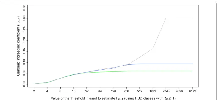
We fitted a Mix14R model using different SNP densities, i.e., from LD (6844 SNPs) to HD (601,226 SNPs) on the 634 BBB dataset and even to WGS (5,653,911 SNPs) for the 50 whole-genome sequenced individuals. Average estimated inbreeding coefficients measured with respect
to different base populations (Fig. 4) and Additional
file 3: Fig. S2 were similar across SNP panels for the most
recent base populations (FG-32). For more ancient base
populations, less autozygosity was captured with the LD panel with marked differences for ancient HBD classes that were captured only with HD or WGS panels. A simi-lar trend was observed with the 50 K panel but average inbreeding coefficients were similar to those from the
HD panel up to FG-256 (approximately 128 generations
back). The average inbreeding coefficients estimated by using the most remote base population and the LD, 50 K and HD panels were equal to 0.060, 0.093 and 0.303,
respectively (when estimated on the 50 sequenced indi-viduals only, these values were equal to 0.047, 0.101 and 0.309, respectively, and to 0.359 with the WGS panel). The base population is then a function of the smallest HBD segments that can be captured by the panel used. The correlations between these inbreeding coefficients estimated with different panels were high, i.e., 0.934 (LD-HD), 0.944 (LD-50 K) and 0.975 (50 K-HD). In spite of the much lower inbreeding coefficients obtained with the 50 K panel, it captures essentially all the individual vari-ation obtained with a HD panel, in agreement with the earlier observation that most of the variation was associ-ated with recent HBD classes.
We then used the Viterbi algorithm to identify HBD
segments with different SNP panels (Table 1). The Viterbi
algorithm classifies each SNP position as HBD or non-HBD whereas the forward-backward algorithm provides the local HBD probability. As expected, more and shorter HBD segments are captured with higher density panels. With the HD panel, a limited proportion of extremely small (a few kb) segments were captured. The length of the majority of the segments ranged from 10 to 500 kb, with more than half being shorter than 100 kb, but such segments do not necessarily have the largest contri-bution to the total percentage of the genome in HBD classes since classes with fewer but longer segments can account for a large proportion of autozygosity. We also observed extremely long HBD segments (> 50 Mb),
0. 00 .1 0.2 0.3 0.4
Genomic inbreeding coefficient (F
G−T
)
2 4 8 16 32 64 128 256 512 1024 2048 4096 8192
Value of the threshold T used to estimate FG−T (using HBD classes with RK≤ T)
ANG BBB BSW CHL GNS HFD HOL JER LMS PMT RMG
Fig. 3 Estimation of inbreeding coefficients with respect to different base populations (the threshold T determines which HBD classes are included in the estimation of FG‑T) with a Mix14R model in 11 cattle breeds of European origin using the BovineHD SNP panel. ANG Angus, BBB Belgian Blue
Beef cattle, BSW Brown Swiss, CHL Charolais, GNS Guernsey, HFD Hereford, HOL Holstein, JER Jersey, LMS Limousin, PMT Piedmontese, RMG Romag‑ nola
which confirmed the presence of recent autozygosity (the longest HBD segment was more than 90 Mb long). On average, each of the 634 bulls had 4.25 HBD seg-ments that were longer than 10 Mb and associated to a common ancestor that was present approximately five generations back. The number of such HBD segments ranged from 0 to 14 per individual. Sixty-one bulls had even one or more (up to three) HBD segments longer than 50 Mb. With the 50 K and LD panels, more than
99% of the identified segments were longer than 100 and 500 kb, respectively (with a peak in the classes from 1 to 5 Mb and from 5 to 10 Mb, respectively), and only a frac-tion of the segments were captured compared to when the HD panel was used. In particular, the vast majority of the HBD segments shorter than 1 Mb were not identified. At lower SNP densities, the smallest segments are sim-ply not captured because they do not contain any SNP or too few. Segments of intermediate size might not reach high HBD probabilities due to a smaller number of SNPs in the segment. Conversely, the length of some HBD seg-ments can be overestimated when using the LD panel, for instance when there are not enough SNPs to iden-tify small non-HBD segments that flank HBD segments.
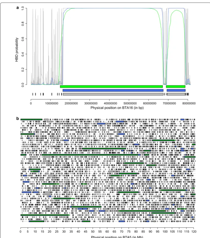
Figure 5a illustrates the identification of HBD segments
for one chromosome. It shows that (1) more segments were identified at higher density, (2) HBD probabilities were higher with denser maps, (3) the Viterbi algorithm declared some SNP positions as HBD although they had only moderate HBD probabilities, and (4) the boundaries of HBD segments varied with the panel density. Similarly,
Fig. 5b represents HBD segments that were identified on
Bos taurus chromosome (BTA) 5 for 50 individuals with the Viterbi algorithm with different SNP densities. The
results are in agreement with those reported in Table 1.
Larger proportions of the genome were declared HBD with the HD panel and small HBD segments accounted for most of the difference with results from lower den-sity panels. Still, we observed that some HBD segments
0.00 0.05 0.10 0.15 0.20 0.25 0.30 0.35
Genomic inbreeding coefficient (F
G−T
)
2 4 8 16 32 64 128 256 512 1024 2048 4096 8192
Value of the threshold T used to estimate FG−T (using HBD classes with RK≤ T)
Fig. 4 Comparison of inbreeding coefficients estimated with different SNP densities (LD panel in green, 50 K panel in blue and BovineHD panel in grey) and for different base populations (the threshold T determines which HBD classes are included in the estimation of FG‑T). Estimation of
inbreeding coefficients was performed with the Mix14R model for 634 Belgian Blue sires
Table 1 Distribution of the length of HBD segments iden-tified with a model with 13 HBD-classes with pre-defined
Rk rates for different SNP densities
HBD segment length
category Panel density
LD panel 50 K panel BovineHD panel
≤1 kb 0 0 17 1–5 kb 0 0 1828 5–10 kb 0 0 16296 10–50 kb 1 10 570179 50–100 kb 3 40 614787 100–500 kb 48 1346 793645 0.5–1 Mb 146 2500 53984 1–5 Mb 1172 11658 25839 5–10 Mb 1728 3201 3189 10–50 Mb 2638 2643 2627 50–100 Mb 74 71 69
Physical position on BTA16 (in bp) HBD probability 0.0 0.2 0.4 0.6 0.8 1.0 0 10000000 20000000 30000000 40000000 50000000 60000000 70000000 80000000 a
Physical position on BTA5 (in Mb)
0 5 10 15 20 25 30 35 40 45 50 55 60 65 70 75 80 85 90 95 100 105 110 115 120
b
Fig. 5 Illustrations of the identification of HBD segments using different SNP panels. a Example of estimated HBD probabilities for one individual on Bos taurus autosome (BTA) 16 using different SNP densities (LD panel in green, 50 K panel in blue and BovineHD panel in grey). The horizontal lines
below the curves represent HBD segments as identified by the Viterbi algorithm with the three panels. An extremely long HBD segment (~ 50 Mb) is represented (there are only 69 such HBD segments identified in the entire data set), suggesting recent inbreeding. This bull is one of the 29 individuals carrying such long HBD segments and has a pedigree inbreeding coefficient of 0.048. b Comparisons of HBD segments identified for 50 individuals on BTA5 using different panels (each line represents one individual). Segments identified with the HD, 50 K and LD panels are repre‑ sented in grey, blue and green, respectively (with lower density results masking results obtained at higher density). The shortest HBD segments are identified with the HD panel (indicated in grey) whereas those of intermediate size are also captured with the 50 K panel (and still missed with the LD panel) and indicated in blue. For a few HBD segments, the use of the LD panel results in longer segments
of a few Mb long were not identified at lower SNP
den-sity (and even more so with the LD panel). As for Fig. 5a,
the length of some HBD segments is overestimated when the LD panel was used. We also compared the local HBD probabilities estimated by using either the LD or the 50 K panel with the local HBD classes inferred by using the
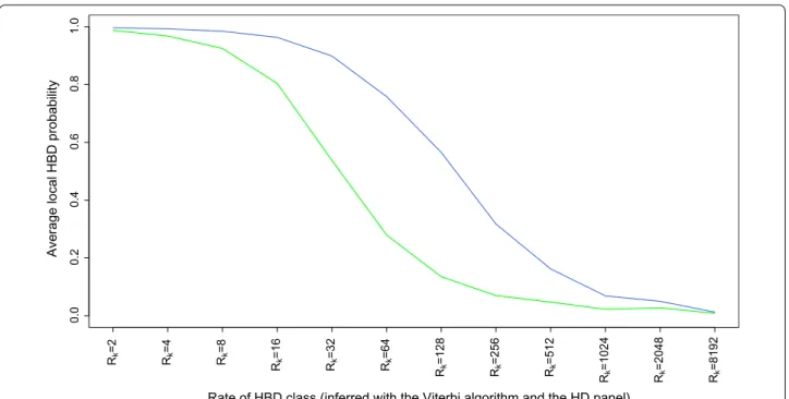
HD panel and the Viterbi algorithm (Fig. 6). HBD
prob-abilities were high for recent HBD classes and dropped for more remote common ancestors. As expected, the LD panel was efficient for only the most recent com-mon ancestors (the HBD probability was 0.90 or higher
when Rk < 16 and ~ 0.50 for Rk = 32) whereas the 50 K
panel allowed the capture of more ancient autozygosity
(the HBD probability was 0.90 or higher when Rk < 64
and ~ 0.50 for Rk = 128). More results regarding the age
(or length) of HBD segments that can be captured with different SNP densities are described in Druet and
Gau-tier [26].
Comparison of models
Models that estimate Rk rates of HBD‑classes (KR models)
For the different SNP densities tested and for each
indi-vidual, we used the BIC (see [26]) to select the KR model
with the best statistical support (i.e., with the optimal number of classes K, with K − 1 HBD classes and one
non-HBD class) after estimating the rate(s) Rk for each
individual with each tested model. For each SNP panel,
Table 2 shows the number of times a model was selected
as the best one for the individual analyzed. As SNP den-sity increases, more past generations can be explored and the optimal K increases accordingly. In most cases, mod-els with one HBD class are preferred for the LD panel, models with two HBD classes for the 50 K panel, mod-els with three HBD classes for the HD and WGS panmod-els (although the model with four HBD classes is also often selected for the latter, i.e., for 23 of 50 individuals). With these optimal models, the first HBD-class captures the
most recent autozygosity (Rk from 15 to 20), the second
HBD-class captures autozygosity that is associated to common ancestors from a few hundred generations back
and later classes are associated with higher Rk (> 1000)
(Table 2). Correlations of inbreeding coefficients
esti-mated with these selected KR models with those obtained with the complete Mix14R model (ranging from 0.981 to 1.000) and comparison of the average estimated inbreeding coefficients indicate that with these reduced KR models, we can effectively capture the genome-wide autozygosity. With 1R models and low or moderate SNP densities, we observed a slight underestimation of the inbreeding coefficients compared to the Mix14R model
and slightly lower correlations (still above 0.98). The Rk
rates estimated for each individual with these panels have a lower median value (respectively 15 and 41 with
the LD and 50 K panels) than the Rk rates estimated with
0. 00 .2 0. 40 .6 0.8 1.0
Average local HBD probability
Rk =2 Rk =4 Rk =8 Rk =1 6 Rk =3 2 Rk =6 4 Rk =128 Rk =256 Rk =512 Rk =1024 Rk =2048 Rk =8192
Rate of HBD class (inferred with the Viterbi algorithm and the HD panel)
Fig. 6 Average HBD probabilities estimated for HBD segments associated with different age‑based classes. HBD probabilities were estimated with the LD (green) or 50 K (blue) panels whereas the age‑based classes were determined by using the Viterbi algorithm and the HD panel (a 20‑fold SNP density increase). The average HBD probabilities indicate whether segments from different classes are captured using lower density panels
higher density panels (median Rk > 1000) for which the
contribution of smaller ROH is much larger. As a result, some small fragments were not captured by the model at lower density whereas at higher density, inbreeding coef-ficients are almost identical to estimates obtained with the Mix14R model. Models containing two or more HBD classes captured the same amount of autozygosity as the Mix14R model, irrespective of SNP density. Although the inbreeding coefficient is correctly estimated with a 1R model (one HBD and non-HBD class with the same rate) with WGS data, the HBD segments identified tend
to be smaller since the estimated Rk rates are higher (i.e.,
smaller expected lengths of fragments) as shown in
Addi-tional file 4: Fig. S3. Indeed, the 1R model results in more
10 to 100 kb long segments than the Mix14R model, but fewer segments longer than 100 kb. Thus, with a 1R model, long HBD segments might be cut into smaller fragments in the presence of heterozygous SNPs (pos-sibly sequencing errors) whereas with models including HBD class(es) associated with recent common ancestors
(with small Rk rates), these HBD segments are
identi-fied as one long and recent fragment (because the
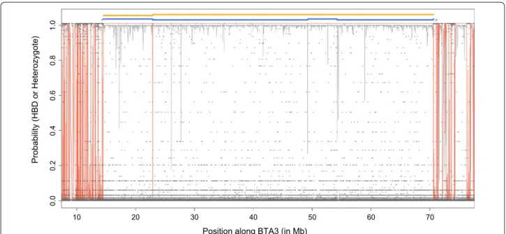
pen-alty to end and start a new segment is higher). Figure 7
illustrates this with an example. Indeed, we observed a long segment with high HBD probabilities although there are multiple positions where the probability of the
heterozygous genotype is non-null (but this is limited compared to flanking regions). With the Mix14R model, this is considered as a long segment and the local HBD probability remains higher than 0.99 for the entire region (except for a region with five consecutive heterozygous SNPs). With the 1R model, the HBD probabilities drop repeatedly due to these possibly heterozygous SNPs and the longest HBD segment is cut into several smaller frag-ments (based on the results from the Viterbi algorithm). Note that with the HD panel, this individual is homozy-gous for all 13,009 SNPs that are included in this 56.1-Mb
long segment. As in Fig. 5, we note that the Viterbi
algo-rithm classifies some positions with a low estimated HBD probability as HBD.
Models with pre‑defined Rk rates of HBD classes (MixKR
models)
Compared to the KR models, MixKR models present the advantage of using the same HBD classes for all
individu-als (Rk rates of HBD classes are not individually estimated
but pre-defined by the user) and make comparisons between individuals easier (for instance, comparing two
individuals with a single HBD class but with Rk = 8 for
the first and Rk = 96 for the second would not be easy –
the estimated Rk range from 4 to 1000). Several of these
MixKR models (with K = 2, 3 and 4) were tested with Table 2 Comparison of models used to estimate genomic inbreeding coefficients with different numbers of HBD classes (from 1 to 4)
The Rk rates of each HBD class were estimated for each individual and for each SNP density (LD, 50 K, HD panels or whole-genome sequence data). The table reports which models are selected as best based on the BIC criterion, the average FG and its correlation with a reference FG obtained with a model using 13 HBD classes a N = number of individuals with the corresponding model selected as best based on the BIC
b The reference inbreeding coefficient F
G-8192 is obtained with a Mix14R model and the same SNP density Panel density Na Number of fitted HBD
classes Mean FG Correlation with F
b
G-8192 Median of estimated Rk rates per HBD class
1st HBD class 2nd HBD class 3rd HBD class 4th HBD class
LD 634 1 0.058 0.982 15 LD 0 2 0.061 0.998 11 106 LD 0 3 0.061 0.999 11 104 162 LD 0 4 0.061 0.999 10 42 150 175 50 K 289 1 0.083 0.983 41 50 K 345 2 0.094 0.999 15 198 50 K 0 3 0.094 1.000 14 173 238 50 K 0 4 0.094 1.000 11 64 240 243 HD 0 1 0.297 0.999 1214 HD 0 2 0.302 1.000 60 1679 HD 629 3 0.303 1.000 22 392 1887 HD 5 4 0.303 1.000 19 342 1823 1914 WGS 0 1 0.354 1.000 3740 WGS 0 2 0.359 1.000 577 8158 WGS 27 3 0.359 1.000 55 1009 8192 WGS 23 4 0.359 1.000 21 206 1104 8192
the LD panel (Table 3) to assess whether reduced mod-els with pre-defined rates of HBD classes are efficient. To select these pre-defined rates, either we used medians of estimated rates obtained from models with the same number of classes (see previous section) or we selected a few classes from the MixKR model in order to cover the range of estimated values (e.g., one class for recent HBD segments and one for ancient HBD segments). In agreement with previous observations on KR models, comparisons of estimated inbreeding coefficients with those obtained with the Mix14R model indicate that models with a single HBD class slightly underestimate the inbreeding coefficients and result in lower correla-tions (> 0.96) than models with two or more HBD classes
(> 0.99). Presence of multiple HBD-classes (> 2) allows better assessment of the contributions from different past
generations (e.g., Rk = 8 vs 64) but does not provide
bet-ter estimates of the genome-wide inbreeding coefficient. Comparison to other inbreeding coefficient estimators Means and ranges of inbreeding coefficients estimated
with different methods and the HD panel are in Table 4
and their correlations are in Table 5, and in Additional
file 5: Tables S1 and S2 for other panels. Similar to our
model, models based on observed homozygosity and ROH resulted in high inbreeding coefficients (respec-tively, 0.644 and 0.151 on average) whereas other genomic estimators resulted in inbreeding coefficients centered
10 20 30 40 50 60 70 0.0 0.2 0.4 0.6 0.8 1.0
Position along BTA3 (in Mb)
Probability (HBD or Heterozygote)
Fig. 7 Comparison of the length of HBD segments identified with WGS data and with the 1R or the Mix14R models on BTA3. The grey and red lines
represent the HBD probabilities estimated with the 1R and Mix14R models, respectively; the dark grey dots represent the probability of heterozy‑
gous genotypes (obtained from the VCF); the blue and yellow segments represent HBD segments identified with the Viterbi algorithm with the 1R and the Mix14R model, respectively
Table 3 Estimation of genomic inbreeding coefficients with models using different numbers of HBD classes (from 1 to 4)
with pre-defined Rk rates that correspond to the expected length in Morgans of HBD segments and with the LD panel
a The reference inbreeding coefficient F
G is obtained with a Mix14R model and the same SNP density
Number of fitted HBD classes Mean FG Correlation with reference FGa Predefined R
k rates used for each HBD class
1st HBD class 2nd HBD class 3rd HBD class
1 0.058 0.967 20
1 0.056 0.963 16
2 0.060 0.996 10 100
2 0.061 0.994 16 256
around 0 and including negative values. It should be noted that higher values are obtained on average (0.268) when using less stringent rules to identify ROH (e.g., windows of 20 SNPs and at least 10 SNPs per ROH). We observed very high correlations between HMM-based estimates and both measures based on homozygosity
(r = 0.95 with FHOM and FExHOM, these two measures
pre-senting a correlation of 1 and being essentially the same)
or on ROH (r = 0.95 with FROH), which suggest that with
large numbers of SNPs, simple heuristics (ignoring allele
frequencies, SNP spacing, etc.) are efficient (FHOM and
FROH being highly correlated, r = 0.97). The correlation
between FHOM estimated with LD and HD panels is equal
to 0.890, which is slightly lower than the correlation between estimates obtained with the HMM for these two panels (r = 0.934), which indicates that global estimators still work properly with 6844 SNPs in this population. Rule-based ROH methods are less efficient at lower SNP densities since they capture only the longest fragments (5 Mb or more and 20 Mb on average) with the param-eters used in the current study (the default windows size in plink). In fact, ROH-based estimators are rarely used with the LD panel in cattle although more HBD seg-ments might be identified with less stringent rules, at the expense of an increased rate of false positives. At low SNP density, the HMM framework still provides correct global and local HBD probabilities although HBD
seg-ments are not identified without ambiguity [26].
Correlations of estimates from the traditional GRM with our estimates are moderately high (r = 0.73) and lower with homozygosity estimators (r = 0.63) and
ROH-based estimators (0.61). The FGRM was computed with the
formula proposed by [13], which divides all SNP
contri-butions by the same weight. When estimated with the alternative formula, which divides each SNP
contribu-tion by its own weight 2fi (1 − fi) (fi being the frequency
of SNP i) as in Amin et al. [42], correlations were lower
(i.e., 0.48 with FG, 0.34 with FHOM and 0.33 with FROH).
The estimator based on the unified correlations between
gametes proposed by Yang et al. [38] presented relatively
high correlations with both FG and FGRM (respectively,
0.90 and 0.92) and slightly lower correlations with the
other estimators (r = 0.87 and 0.85 with FHOM and FROH,
respectively).
Correlations of these estimates with pedigree inbreed-ing coefficients (considerinbreed-ing only individuals born after
1999 to increase pedigree depth) are also in Table 5.
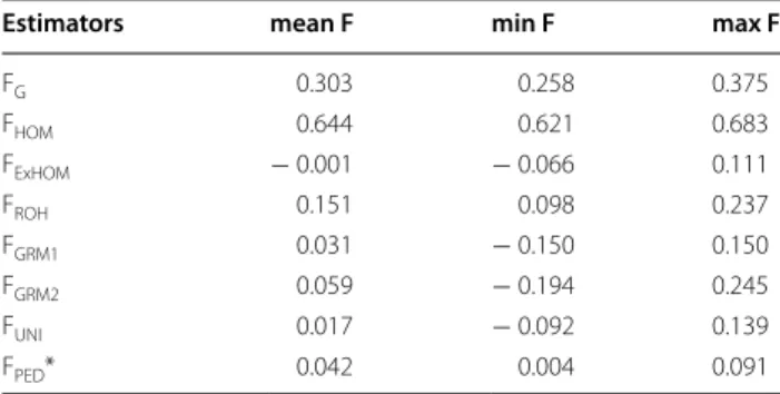
Overall correlations were moderate with the highest Table 4 Summary statistics for the inbreeding coefficients
estimated for the 634 Belgian Blue sires with different methods and using the HD panel
FG, inbreeding coefficient estimated as the probability of belonging to any of the HBD classes averaged over the whole genome; FHOM, inbreeding coefficient based on the proportion of homozygous SNPs; FExHOM, excess homozygosity estimator; FROH, inbreeding coefficient estimated as the proportion of the genome captured by ROH; FGRM1, inbreeding coefficient based on the diagonal elements of the genomic relationship matrix (dividing all SNP contributions by the same denominator); FGRM2, inbreeding coefficient based on the diagonal elements of the genomic relationship matrix (dividing each SNP contribution by its own weight 2fi (1 − fi), fi being the frequency of allele i); FUNI, inbreeding coefficient based on the correlation between uniting gametes; FPED, inbreeding coefficient estimated from pedigree data
*Estimated on the 313 bulls born after 1999
Estimators mean F min F max F
FG 0.303 0.258 0.375 FHOM 0.644 0.621 0.683 FExHOM − 0.001 − 0.066 0.111 FROH 0.151 0.098 0.237 FGRM1 0.031 − 0.150 0.150 FGRM2 0.059 − 0.194 0.245 FUNI 0.017 − 0.092 0.139 FPED* 0.042 0.004 0.091
Table 5 Correlations between inbreeding coefficients estimated for the 634 Belgian Blue sires with different methods and using the HD panel
FG, inbreeding coefficient estimated as the probability of belonging to any of the HBD classes averaged over the whole genome; FHOM, inbreeding coefficient based on the proportion of homozygous SNPs; FExHOM, excess homozygosity estimator; FROH, inbreeding coefficient estimated as the proportion of the genome captured by ROH; FGRM1, inbreeding coefficient based on the diagonal elements of the genomic relationship matrix (dividing all SNP contributions by the same denominator); FGRM2, inbreeding coefficient based on the diagonal elements of the genomic relationship matrix (dividing each SNP contribution by its own weight 2fi (1 − fi), fi being the frequency of allele i); FUNI, inbreeding coefficient based on the correlation between uniting gametes; FPED, inbreeding coefficient estimated from pedigree data
FHOM FExHOM FROH FGRM1 FGRM2 FUNI FPED
FG 0.948 0.945 0.945 0.730 0.481 0.905 0.463 FHOM 0.999 0.974 0.627 0.343 0.873 0.546 FExHOM 0.974 0.633 0.351 0.878 0.547 FROH 0.610 0.328 0.853 0.551 FGRM1 0.938 0.917 0.286 FGRM2 0.748 0.091 FUNI 0.454
values for correlations with homozygosity and ROH-based measures (0.55 for both measures) and slightly lower values for those with the HMM-based estimator
(0.46), whereas we observed a low relationship with FGRM
(0.29) and a moderate correlation with FUNI (0.45). We
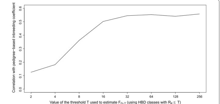
also compared the FPED and inbreeding coefficients
esti-mated with our model with respect to different base
pop-ulations (Fig. 8) and found that correlations increased up
to FG-32 (capturing the inbreeding from ancestors
approx-imately 16 generations back) and then presented a
pla-teau from FG-32 to FG-256 reaching a maximum at r = 0.56
(i.e., slightly better than homozygosity-based
estima-tors). This trend was expected since FPED is estimated for
a limited number of generations back in time. The aver-age equivalent number of known generations estimated
with PEDIG [43] was 6.3 for the bulls born after 1999
(it increased from 5.5 for bulls born in 2000 to 7.5 for
those born in 2010) corresponding on average to FG-16.
The addition of HBD-class Rk = 32 allows the capture of
contributions from some older branches of the pedigree and the smallest HBD segments inherited from common ancestors in the pedigree.
Discussion
For several reasons, the Belgian Blue Beef cattle breed is considered as an extremely selected breed. It is famous for its exceptional muscular development referred to as
“double muscling”, which is caused by an 11-bp deletion
in the myostatin gene [44]. This loss-of-function variant
is almost fixed in the current population (e.g., [45]) but
muscular development was further improved through
intense selection [46]. As a result, most often calving
requires caesarian section. In addition, artificial insemi-nation is more frequent in this breed compared to other beef cattle breeds, which allows a more intense use of key sires. In recent years, several outbursts of recessive defects associated with inbreeding have been reported. For instance, causative variants were identified for eight recessive defects including congenital muscular dystonia
1 and 2 [5], crooked tail syndrome [6, 7], stunted growth
[8], gingival hamartome [9], prolonged gestation, lethal
arthrogryposis syndrome [10] and junctional
epidermol-ysis bullosa [11]. Some of these defects have reached a
high frequency in the population.
When estimated over all HBD-classes, the average genomic inbreeding coefficient was high (higher than 0.30) but these values were comparable to those obtained for other cattle breeds of European origin (i.e., BBB pre-sented intermediate values). In agreement with Purfield
et al. [22], samples from breeds that originated from the
British Isles (Hereford, Angus, Jersey or Guernsey) pre-sented high inbreeding coefficients (≈ 34 to 40%), pos-sibly as a result of closed population histories and strict
importation restrictions [22]. Similarly, high levels of
0.0 0.1 0.2 0. 30 .4 0. 50 .6
Correlation with pedigree−based inbreeding coefficient
2 4 8 16 32 64 128 256
Value of the threshold T used to estimate FG−T (using HBD classes with RK≤ T)
Fig. 8 Correlations between the inbreeding coefficients estimated with respect to different base populations (FG‑T) and the inbreeding coefficient
estimated from pedigree data for the Belgian Blue sires born after 1999 and using the HD panel. Different base populations were obtained by selecting different thresholds T that determine which HBD‑classes are considered for estimating FG‑T (e.g., setting the base population approxi‑
mately 0.5 * T generations in the past). The corresponding inbreeding coefficients FG‑T are estimated as the probability of belonging to any of the
inbreeding in Holstein and Brown Swiss breeds were
pre-viously reported [21, 41, 47]. When focusing on recent
common ancestors only (associated with HBD-classes
with Rk ≤ 64), we observed lower inbreeding coefficients
in BBB cattle, ranging from 1.0 to 17.7% across animals (6.8% on average), with a positive trend: animals from the current population presenting 6% higher inbreeding coefficients on average than individuals born 30 years ago. Some individuals accumulated more than 10% recent autozygosity and carried HBD segments longer than 10 or even 50 Mb. The same model applied to other species, i.e., dog breeds or sheep populations that suf-fered severe bottlenecks revealed significantly higher
lev-els of recent autozygosity [26]. Conversely, some human
and sheep populations presented lower levels of recent autozygosity (even lower than 1% on average). The recent HBD-classes are probably more relevant for management purposes because they account for most of the individual variation in genome-wide autozygosity. In addition, del-eterious variants might be mostly associated to recent HBD segments because older variants have undergone more generations of selection against deleterious effects
(e.g., [3, 48, 49]). Recent intensive selection of key sires
allowed some deleterious variants to reach higher fre-quency than under natural selection. Indeed, strong bot-tlenecks that occur with domestication, breed creation or intensive selection in cattle result in the relaxation of purifying selection and increase the load of deleterious
mutations (e.g., [50, 51]). For instance, all identified
vari-ants that cause recessive defects in BBB cattle are specific to this breed (suggesting their young age). We applied
our model to previously genotyped cases (see [52]) and
the causative variants were found on recent HBD
seg-ments (associated with HBD-classes with Rk ≤ 32), also
suggesting that these variants are relatively young. Application of our model with different SNP densities showed large differences in average estimated
inbreed-ing coefficients, with the average FG equal to 0.060, 0.093
and 0.303 using the LD, 50 K and HD panel, respec-tively. Correlations between these estimates were very high (even with the LD panel, r > 0.93). High-density panels allow the capture of shorter ROH that are asso-ciated with very ancient ancestors, are characteristic of the population (associated with past demographic his-tory) and present little individual variation. For recent HBD classes, estimators were similar across SNP
pan-els (up to Rk = 32 with the LD panel and 256 with the
50 K panel). Small HBD segments, ranging from 10 kb to 1 Mb, accounted for most of the differences obtained with the HD panel compared to the lower density panels. A substantial proportion of HBD segments longer than respectively 1 and 5 Mb were identified with the LD and the 50 K panels. These observations are consistent with
those of Ferenčaković et al. [20] and Purfield et al. [22]
who showed that denser panels can be used to identify short ROH and that the 50 K panel proved suitable to identify ROH longer than 5 Mb. If the goal is to estimate the inbreeding coefficient with respect to a recent base population, which has more variation and is possibly the most functionally relevant one (see above), these LD and 50 K panels provide enough information (e.g., the
corre-lation between FG estimated with the HD and the 50 K
panels was equal to 0.975). Regarding the optimal model, our comparisons indicated that models with a few HBD classes (1 or 2 according to SNP density) achieved results that were as good as those obtained with 13 HBD classes
in terms of FG and correlations with more complex
mod-els. Thus, such parsimonious models were selected based on the BIC. For each SNP panel, we recommend the use of the largest K that is optimal for a substantial propor-tion of individuals since that value is required for these animals and using a larger K will not penalize the other individuals. To make comparisons between individuals easier, we also recommend the use of a model with
pre-defined Rk rates and the same HBD-classes for all
indi-viduals. In that case, the use of at least two HBD-classes is preferable with low-density panels, one to capture the recent HBD segments and one that is associated with more remote ancestors. Three HBD-classes models pre-sent a parsimonious solution to distinguish recent from
ancient autozygosity (similarly to [16]) but if the objective
is to obtain a finer age-based partitioning of autozygosity, more HBD classes could be recommended.
Comparisons of inbreeding coefficients obtained with different estimators have already been reported in the literature. In this paper, we also report correlations with our estimates of genome-wide inbreeding. These com-parisons are essentially indicative since different methods refer to different base populations and all estimators are
not fully comparable (e.g., [53]). In addition, some
esti-mators are sensitive to the estimated allelic frequencies. Here, we used frequencies that were estimated using the set of genotyped bulls born before 1985. At moderate to high SNP density, the genome-wide inbreeding coeffi-cient estimated with our model, averaged over all SNPs and HBD classes, was highly correlated with homozygo-sity measures or ROH-based estimates, whereas lower correlations were obtained when compared to estimates based on the genomic relationship matrix. Low
cor-relations between FGRM and homozygosity measures
(homozygosity or ROH) were previously reported (e.g.,
[54]) although moderate to high correlations were also
found (e.g., [2, 4]). It should be kept in mind that these
results must be interpreted with caution because global
estimators, and particularly FGRM, depend strongly on
addition to global inbreeding coefficients, our model also estimates local autozygosity (i.e., it identifies HBD seg-ments) and uses the linkage between SNPs as ROH-based estimators, conversely to global estimators that consider
all SNPs as independent (FHOM, FGRM, FUNI or FPED).
Cor-relations with homozygosity measures decreased at lower SNP densities when the use of linkage between succes-sive SNP positions was more important to determine whether a position is IBD or not. ROH-based estimators are not frequently used with LD panels in cattle and pre-vious studies concluded that LD panels were appropriate to identify recent inbreeding or HBD segments longer
than 5 Mb [20, 22]. The HMM proved to work well with
LD panels, i.e., it captured the recent HBD segments, presented high correlations with coefficients estimated at higher density, and provided HBD probabilities. It is indeed recommended to use such probabilities at low-density because they account for uncertainty due to lower informativeness as opposed to ROH-based classification or the Viterbi algorithm. We showed that, at lower SNP densities, the smallest HBD segments are not captured but also that the Viterbi algorithm even fails to identify some segments of moderate size. Therefore, we recom-mend the use of HBD probabilities that are obtained with the forward-backward algorithm. Most of the global estimators provided inbreeding coefficients relative to a base population, i.e., the founders of the pedigree or the population used to estimate allele frequencies, whereas the multiple-HBD class model provides an age-based partitioning of autozygosity. As a result, inbreeding coefficients estimated by including all HBD classes are higher because some HBD-classes trace back to more remote generations than the base population commonly used by other methods and the SNP density determines how ancient HBD segments can be captured. Compared to rule-based ROH, the HMM framework also allows to accommodate low-fold sequencing or genotype-by-sequencing data, i.e., when genotypes are not
unambigu-ously determined, as described in Vieira et al. [25] and
Druet and Gautier [26].
Moderate to high correlations between FPED and FROH
(from 0.50 to 0.75) were reported in cattle (e.g., [3, 21,
22, 54, 55]). In addition, long ROH (> 5 Mb) were shown
to be closely associated with pedigree inbreeding
coef-ficients [22]. Correlations between estimators obtained
from the pedigree and the genomic relationship matrices
are more variable, ranging from moderate (e.g., [4]) to
high (e.g., [37]), whereas in other studies, these
correla-tions were particularly low [54, 56]. As mentioned above,
these differences might be due to the estimation of the allelic frequencies. Inbreeding coefficients estimated with the HMM had moderate correlations with pedigree-based inbreeding coefficients, lower than with methods based on homozygosity or ROH that were in the range with cor-relations reported in previous studies. However, correla-tions were higher with the autozygosity associated to the recent HBD-classes, which is a desired feature since these recent classes correspond to the autozygosity captured by the pedigree whereas old HBD-classes are associated to ancestors tracing further back than the genealogy. Simi-larly, correlations between HMM inbreeding coefficients estimated with the LD panel and pedigree-based esti-mates were higher since they capture only recent autozy-gosity (compared to higher density panels).
Conclusions
Although we observed high levels of inbreeding asso-ciated with small HBD segments in Belgian Blue Beef cattle, recent HBD segments account for most of the individual variation. Recent autozygosity can be cap-tured efficiently with low-density SNP panels and with relatively simple models (e.g., two HBD classes) although
we recommend the use of models with pre-defined Rk
rates that are associated with the expected length of HBD segments (the same HBD-classes are then used for all individuals) to make comparisons between individuals easier. More complex models (with more age-based HBD classes) are needed to obtain a finer age-based partition-ing of inbreedpartition-ing levels and indications of the past demo-graphic history of a population. Such partitioning allows to better understand which HBD classes contribute to individual autozygosity. In addition, the use of more classes avoids the fragmentation of long HBD segments into smaller fragments with next-generation sequenc-ing data. Estimates obtained with the HMM framework are highly correlated with those obtained based on rela-tive homozygosity (or ROH). In addition, such HMM can use genotype probabilities (e.g., with low-fold sequencing data) and provide, beyond global estimates, local HBD probabilities that are still useful at lower SNP densities. Such local HBD probabilities might be useful to identify regions associated with inbreeding depression.
Additional files
Additional file 1. Figure S1. Trend per year of birth of individual inbreeding coefficients in the 634 Belgian Blue sires. Inbreeding coeffi‑ cients were estimated with the Mix14R model (13 HBD‑classes model with pre‑defined Rk rates) using the BovineHD genotyping panel. (a) Trend for
genomic inbreeding coefficients estimated using all HBD classes; (b) trend for genomic inbreeding coefficients estimated with the most recent HBD classes (Rk ≤ 32) and (c) trend obtained with pedigree‑based estimates. Additional file 2. Boxplots of proportions of individual genomes associ‑ ated with 13 HBD‑classes with pre‑defined Rk rates (MIX14R model) in 11
cattle breeds of European origin using the BovineHD genotyping panel. The proportions correspond to individual genome‑wide probabilities of belonging to each of the HBD‑classes.
Additional file 3. Figure S2. Comparison of genomic inbreeding coef‑ ficients estimated with different marker densities (LD panel in black, 50 K panel in red, BovineHD panel in green and WGS panel in blue) and for dif‑ ferent base populations. Genomic inbreeding coefficients were estimated with the Mix14R model (13 HBD‑classes model with pre‑defined Rk rates) for 634 Belgian Blue sires. Different base populations were obtained by selecting different thresholds T that determine which HBD‑classes were considered in the estimation of FG‑T (e.g., setting the base population
approximately 0.5 * T generations in the past).
Additional file 4. Figure S3. Distribution of length of HBD segments identified with whole‑genome sequence data and using models with different numbers of HBD classes.
Additional file 5. Table S1. Correlation coefficients between inbreeding coefficients estimated with different methods for the 634 Belgian Blue sires and using the 50 K panel. The table reports the correlations between all inbreeding coefficients estimated with different methods using the 50 K panel. Table S2. Correlation coefficients between inbreeding coef‑ ficients estimated with different methods for the 634 Belgian Blue sires and using the LD panel. The table reports the correlations between all inbreeding coefficients estimated with different methods using the LD panel.