Un modele vibroacoustique pour prevoir l’effet de niche sur la perte par transmission sonore

(1)

UNIVERSITE DE SHERBROOKE Faculte de genie

Departement de genie Mecanique

UN MODELE VIBROACOUSTIQUE POUR

PREVOIR L’EFFET DE NICHE SUR LA PERTE PAR

TRANSMISSION SONORE

Memoire de maitrise Speciality : Genie Mecanique

Mohammad Sadegh G H O LAM I

Jury : Noureddine A TA LLA (directeur) Franck SGARD

(2)

1+1

Library and Archives Canada Published Heritage Branch Bibliotheque et Archives Canada Direction du Patrimoine de I'edition 395 Wellington Street Ottawa ON K 1A0N 4 Canada 395, rue Wellington Ottawa ON K1A 0N4 Canada

Your file Votre reference ISBN: 978-0-494-96276-3 Our file Notre reference ISBN: 978-0-494-96276-3

NOTICE:

The author has granted a non

exclusive license allowing Library and Archives Canada to reproduce, publish, archive, preserve, conserve, communicate to the public by

telecomm unication or on the Internet, loan, distrbute and sell theses

worldwide, for commercial or non commercial purposes, in microform, paper, electronic and/or any other formats.

AVIS:

L'auteur a accorde une licence non exclusive permettant a la Bibliotheque et Archives Canada de reproduire, publier, archiver, sauvegarder, conserver, transmettre au public par telecomm unication ou par I'lnternet, preter, distribuer et vendre des theses partout dans le monde, a des fins com merciales ou autres, sur support microforme, papier, electronique et/ou autres formats.

The author retains copyright ownership and moral rights in this thesis. Neither the thesis nor substantial extracts from it may be printed or otherwise reproduced without the author's permission.

L'auteur conserve la propriete du droit d'auteur et des droits moraux qui protege cette these. Ni la these ni des extraits substantiels de celle-ci ne doivent etre imprimes ou autrement

reproduits sans son autorisation.

In compliance with the Canadian Privacy A ct some supporting forms may have been removed from this thesis.

W hile these forms may be included in the document page count, their removal does not represent any loss of content from the thesis.

Conform em ent a la loi canadienne sur la protection de la vie privee, quelques

form ulaires secondaires ont ete enleves de cette these.

Bien que ces form ulaires aient inclus dans la pagination, il n'y aura aucun contenu manquant.

(3)

UNIVERSITE DE SHERBROOKE Faculty de gdnie

Departement de g6nie Mecanique

VIBRO-ACOUSTIC MODEL TO PREDICT NICHE

EFFECT ON SOUND TRANSMISSION LOSS

Mdmoire de maitrise Sp£cialit£: G&iie Mecanique

Mohammad Sadegh GHOLAM I

Jury : Noureddine ATALLA (directeur) Franck SGARD

Raymond PANNETON

(4)

R6sum6

La r£p£tabilit£ et la reproductibilite sont les probldmes les plus communlment rencontres dans les etudes experimentales de pertes par transmission. Des differences significatives ont ete observees, dans differents laboratoires, sur des mesures de perte par transmission sonore de systemes installs dans une niche (tunnel separant la source des pieces receptrices). Ces essais comparatifs inter-laboratoires ont trouve que la perte par transmission sonore est influencee, non seulement par la plaque, la source et les parametres recepteurs, mais aussi par la profondeur de niche et la localisation de la plaque dans celle-ci.

L’objectif principal de ce travail est de developper et de valider une methode semi-analytique qui soit & la fois rapide, en comparaison avec les methodes des elements finis et des elements de frontiere, et fiable afin d’etudier l’effet de la niche sur la perte par transmission sonore. Ainsi, une methode semi-analytique est proposee et utilisee porn investiguer l’effet de plusieurs parametres de niche sur la perte par transmission sonore d’une fine plaque eiastique. Dans cette etude, deux probiemes seront investigues. Le premier traite de la niche sans plaque dans celle-ci, appeie « aperture ». Le second traite de l’effet de la niche sur la perte par transmission sonore d’une plaque baffiee.

Les ondes acoustiques dans la niche sont developpees en termes de modes acoustiques evanescents et propagatifs. Plusieurs exemples sont presentes pour etudier la convergence et valider l’approche. Les d6couvertes montrent une d^croissance considerable dans la puissance transmise lorsque la longueur de niche augmente. De plus, la longueur de niche joue un role important dans la transmission sonore compare k la surface de section transverse de celle-ci. Dans le syst&me niche-plaque, la niche affecte le champ d’excitation en augmentant la pression sur la plaque. L’augmentation de pression est plus importante au niveau des angles et des aretes de la plaque. Nos r£sultats d’etude rdv^lent que la niche a plus d’effet sur le champ d’excitation que sur le champ de radiation. Ceci est important pour les essais exp&imentaux ou le champ source est mesurg dans une chambre reverberant. Un minimum de perte par transmission sonore, en comparaison avec d’autres positions de plaque dans la niche, est obtenu lorsque la plaque est situee au centre de la niche. Par consequent, l’effet de niche est moins important quand la plaque est situee des le debut de la niche.

Mots-cies: Vibroacoustique, L’effet de niche, La perte par transmission sonore, La methode semi-analytique, L’effet d’aperture.

(5)

Resume English

Repeatability and reproducibility are most common problems in experimental transmission loss studies. Significant differences have been seen in the measurement of sound transmission loss of systems installed in a niche (tunnel separating the source and receiving rooms) in different laboratories. These round robin tests found that sound transmission loss is influenced by not only the plate, source and receiving parameters but also by niche depth and the location of the plate within it.

The main objective of this work is to develop and validate a fast, in comparison with finite element and boundary element methods, and reliable semi-analytical method to study the effect of niche on sound transmission loss. So, a semi-analytical method is proposed and used to investigate the effect of various niche parameters on sound transmission loss of a thin elastic plate. In this study two problems will be investigated. The first deals with the niche without plate inside it which is called “aperture”. The second deals with the effect of niche on sound transmission loss of baffled plate.

The acoustic waves inside the niche are expanded in terms of evanescent and propagating acoustical modes. Various examples are presented to study the convergence and to validate the approach. Findings show considerable decrease in transmitted power as the length of the niche increases. Moreover, niche’s length plays more important role in sound transmission compared to its cross section area. In niche-plate system, niche affects the excitation field by increasing the pressure over the plate. This increase of pressure is more considerable at comers and edges of the plate. Our study results reveal that niche has more effect on excitation field than radiation field. This is important for experimental tests where the source field is measured in a reverberant room. Minimum sound transmission loss, in comparison with other plate position inside the niche, is obtained when the plate is placed at the center of the niche. In this case, niche affects both exciting and radiation fields and because of geometrical symmetry maximum transmission happens at this position. Consequently the niche effect is less considerable when plate is placed at the front side of the niche.

Keywords: Vibro-acoustic, Niche effect, Sound transmission loss, Semi-analytical model, Aperture effect.

(6)

Acknowledgment

It is with immense appreciation that I acknowledge the support and help o f my supervisor, Professor Noureddine Atalla, for his excellent guidance, caring, patience, and providing me with an excellent atmosphere for doing research. Without his guidance and persistent help this dissertation would not have been possible.

I would like to appreciate Professor Frank Sgard and Celse Kafui Amddin whom I learned a lot from them during this study.

(7)

Table of Figures

Figure 1.1: Specimen mounted inside an aperture... 2

Figure 1.2: Possibility o f plate position inside aperture...2

Figure 2.1: Niche and plate configuration. Plate is placed inside the niche... 7

Figure 2.2: Three different position of plate inside niche; a) plate placed in front of the niche, b) Plate placed at the center, c) Plate placed in back side of the niche...8

Figure 2.3: Effect o f specimen position, on STL. ^ is normalized location of the panel at a given frequency below the coincidence frequency o f the plate... 9

Figure 2.4: Niche depth definition for three different lengths; L is the depth and d is the depth of reference niche (a); a) normal depth, b) depth is increased, c) depth is decreased... 10

Figure 2.5: Effect of angled baffle; a) 0=270; b) 0=240; c) 0=90... 10

Figure 3.1: Configuration o f the problem; left to right, angles of incident plane wave, pressure definition and coordinate definition...14

Figure 3.2: Outward normal vector definition for Rayleigh integral... 16

Figure 3.3: System interfaces, from left to right: interface between source & niche, niche, niche and receiving... 17

Figure 3.4: Convergence study, the effect of keeping modes up to two times of truncation frequency... 24

Figure 3.5: Comparison of presented method and FEM-BEM. Normal incident (6 i = 0°

,<pi = 0°) transmission loss of rectangular aperture (b/a=l/2, d /a= l)... 26

Figure 3.6: Comparison o f presented method and FEM-BEM. Oblique incident (9 i = 4 5 °, <pi = 60°) transmission loss of rectangular aperture (b/a=l/2, d /a= l)...26

(11)

Figure 3.7: Effect of niche-depth on STL under plane wave excitation field... ;....28

Figure 3.8: Effect of niche-depth on STL under DAF excitation field...28

Figure 3.9: Effect of increasing the depth up to two and three times under plane wave excitation. The reference system depth is d/a=0.5... 29

Figure 3.10: Effect o f excitation field on STL shown in 1/3 octave band...29

Figure 3.11: Effect o f cross section area on STL... 30

Figure 4.1: System configuration. Left to right: acoustic wave number projection, source side, niche, plate, niche, receiving side, niche dimensions... 34

Figure 4.2: System interfaces, left to right: interface between source & niche, niche & plate, plate &niche and niche and receiving... 34

Figure 4.3: Effect of number o f modes on convergence of STL, plane wave acoustic field. ...48

Figure 4.4: The effect o f number o f modes on convergence o f a) or, b) n t , plane wave

acoustic field...48

Figure 4.5: The effect o f number of modes on convergence of STL, Diffuse acoustic field. ...49

Figure 4.6: Effect o f number modes on convergence o f a) Or, b) n t, Diffuse acoustic field. .49

Figure 4.7: Convergence of the model in NOVAFEM for 6, 8 and 12 elments per wavelength. ...50

Figure 4.8: Validation o f proposed method; Transmission loss o f niche-pate system under oblique plane wave excitation... 51

Figure 4.9: Validation of proposed method, diffuse acoustic field excitation, a) Plate placed at the center o f the niche, b) Plate is flushed mounted at the front side o f their niche...52

(12)

Figure 4.11: STL average in 1/3 octave band, plate is placed at the back side o f the niche 54

Figure 4.12: Niche effect average in 1/3 octave band, plate is placed at back side of the niche.

... 54

Figure 4.13: Transmitted power through the plate... 55

Figure 4.14: Radiation efficiency, plate is placed at the back side o f the niche; a) Narrow band, b) 1/3 Octave band...56

Figure 4.15: Mean square velocity, plate is placed at the back side o f the niche... 56

Figure 4.16: Effect of total pressure over the blocked pressure when d/a=l/3... 57

Figure 4.17: Effect of niche on total pressure... 58

Figure 4.18: Pressure inside the niche, at three points: center, edge and comer; a) Narrow band, b) 1/3 Octave band... 59

Figure 4.19: Effect o f niche depth on total pressure; a) Narrow band, b) 1/3 Octave band 61 Figure 4.20: Effect o f niche-depth on STL... 61

Figure 4.21: Niche effect for three different lengths; a) Narrow band, b) 1/3 Octave band 62 Figure 4.22: Effect o f niche on radiation field... 63

Figure 4.23: STL of the niche and plate, plate is placed at front side o f the niche; a) Narrow band, b) 1/3 Octave band...63

Figure 4.24: Average mean square velocity, plate is placed at front side o f the niche... 64

Figure 4.25: Effect of niche on radiation efficiency, plate is placed at front side of the niche; a) Narrow band, b) 1/3 Octave band...65

(13)

Figure 4.27: Effect o f niche length on niche effect frequency range; a) Narrow band, b) 1/3

Octave band... 66

Figure 4.28: Effect of niche depth on radiation efficiency o f the plate which is placed at front side of the niche; a) Narrow band, b) 1/3 Octave band...67

Figure 4.29:Niche affects both exciting and rcieving side...67

Figure 4.30: Effect o f plate position on STL... ... 68

Figure 4.31: Effect o f plate position on STL... 68

Figure 4.32: Effect of plate position on niche effect; a) Narrow band, b) 1/3 Octave band...69

Figure 4.33: Effec o f plate position inside the niche at different frequencies; a) STL, b) IL. .69 Figure 4.34 : Effect of niche depth on STL... 70

Figure 4.35: Effect of niche depth on STL; a) Narrow band, b) 1/3 Octave band... 71

Figure 4.36: Niche effect. The length of the niche is d/a=l/3, plate placed at x/d=l/2; a) Narrow band, b) 1/3 Octave band... 71

(14)

List of Tables

Table 3.1: Characteristics of aperture... 23

Table 3.2: Excitation field characteristics... 24

Table 3.3: Number of elements for the aperture modeled in N O V A FE M ...25

Table 4.1: The dimensions of niche, plate and plate position inside the niche:...46

Table 4.2: Fluid characteristics:... 46

Table 4.3: Plate mechanical characteristics... 46

Table 4.4: Excitation characteristics for niche-plate system...47

Table 4.5: Dimension and number o f elements for the niche and plate in N O V A FE M ...51

(15)

List of Acronyms

Technical term Definition

BEM Boundary Element Method

DAF Diffuse Acoustic Field

FEM Finite Element Method

GAUS Group d’Acoustique de 1’University de Sherbrooke

IL Insertion Loss

SIF Semi-Infinite Fluid

(16)

List of Variables and Symbols

Symbol Definition

a, b,d Opening dimension and depth of the niche

B' Complex bending stiffness Ci Sound velocity in each sun region E Young's modulus

fc Critical frequency of the baffled plate h Plate thickness

i Imaginary number of module, j = V —1

ko Acoustic wave number k b Bending wave number

ki,pq Wave number in niche 2 and 3

k x<ky> k% Wave number projections in x, y and z direction

m Mass of the plate

P1.P2.P3.P4 Pressure in each sub region

Vb Blocked pressure Pine Incident pressure Pr Radiated pressure PR Reflected pressure

S, Si, S2 Surface area

Ui.n Normal velocity Vs Volume of the plate W {x, y,z ) Displacement field

Plate position

6, <p,r Spherical coordinates Qlim Limit angle

X X X Acoustical wavelength, acoustical wave length in x-y plane, in z

/la* ^xy*Az _direction V Poison ratio

f Normalized plate position inside the niche pi Fluid density in each sub region

T Transmission coefficient

Tdiff Transmission coefficient in diffuse field

(17)

CHAPTER 1 INTRODUCTION

1.1 References

This research is done under supervision of Professor N. Atalla at “Group d’Acoustique de l’Universitd de Sherbrooke (GAUS)”. This study is a part of wider AUT021 funded project attempting to study the acoustical behavior o f niche systems which plays an important role in noise measurements passing through baffled plate between anechoic and reverberant rooms.

1.2 Technological problem

In recent years comprehensive research, on theoretical as well as experimental basis, has been done for the airborne sound transmission through a baffled specimen. In theoretical studies, the thickness of infinite or finite baffle is assumed to be the same as thickness of finite specimen. Consequently, the baffle and specimen, i.e. plate, are coplanar, but this hypothesis is not valid any more in experimental studies. Generally, in order to create a baffle in the lab, a mounting frame (test window) made up from several layers o f isolators and insulators should be installed inside the wall between reverberant and anechoic rooms. So, the test window is considerably thicker than specimen as shown in Figure 1.1. This difference in thickness affects the acoustical behaviour of the specimen when it is large compared to acoustic wave length. In addition, in this new configuration of baffle, there is the variety o f specimen position. Experimental reports show that this parameter also affects the sound transmission loss (STL) measurements.

Because of these reasons different results are obtained at different test facilities, even when the same panels are tested. The term “Niche Effect” is used to refer to the discrepancies caused by the above mentioned reasons. So, niche effect is known as responsible for the inconsistency of low frequency sound transmission measurements. Another possible reason for the discrepancies is the acoustic field in reverberation room where at low frequency range, the model behaviour of room and specimen can affect the STL measurement (Vinokur, 2006). So,

(18)

such large differences in reproducibility haven’t put the reliability of sound transmission loss beyond doubt.

Figure 1.1: Specimen mounted inside an aperture.

Niche effect is considerable when niche with a depth comparable to the acoustic wave length behaves like an acoustic duct. Then, the pressure field inside the niche alters the structural response of the specimen. Several experimental studies (Halliwell & Wamock, 1985) and (Vinokur, 2006) reported that the difference in measured sound transmission loss of the system is related to the plate position inside the niche, Figure 1.2 . In addition other parameters such as tunnel depth and specimen size and shape affect the STL of the system.

(19)

1.3 Scientific problem

General numerical methods such as finite element method (FEM ) or hybrid finite element- boundary element method (FEM-BEM) can be used to study the niche effect. Studying the niche effect while neglecting the effect of acoustic modes of reverberation and receiving rooms means that niche should be connected to semi-infinite fluid (SIF) on each side. The lacks of memory and calculation time problems arise when maximum frequency increases. Accordingly, the main technological objective in this work is to investigate the effect of niche and variation of sound transmission loss with the parameters of panel location, tunnel depth, and panel size using a fast, compared to FEM-BEM, semi-analytical method. Hence, the following query is the open scientific question for this study;

“What is the effect of a niche and its parameters on the sound transmission loss of a baffled panel?”

1.4 Objective

The aim of this study is to extend and validate a fast, in comparison with finite element and boundary element methods, semi analytical method to study the effect o f niche on STL. Two problems w ill be investigated. The first deals with the niche without plate inside it, which is called “aperture”. The second deals with the effect of niche on STL of baffled plate. To this end, following tasks are designed:

1.4.1 Task (I): Literature review

Conduct a literature review on previous works which are related to the topics of this work.

1.4.2 Task (II): Effect of aperture oh STL

Review and validate the semi-analytical method for the niche without plate and provide the reader with numerical results regarding the effect o f length and cross section area o f the

(20)

1.4.3 Task (III): Effect of niche on STL of baffled plate

Propos a general and efficient semi-analytical method to predict both plane wave and diffuse acoustic field (DAF) sound transmission loss of aperture of rectangular cross section. Validate the numerical results with existing in-house code, NOVAFEM.

1.4.4 Task (IV): Effect of niche parameters on STL

Investigate the effect of niche length on STL of the plate and the effect o f plate position inside the niche on STL.

l.S Summary

In this chapter the problematic, objectives and open scientific question were introduced. In addition the main objectives of this study were detailed. As mentioned, the niche effect is associated with the difference in thickness of specimen and baffle. This effect is known as reason of difference in STL measurements in different labs with the same conditions for tests. Chapter 2 presents a review of literature on previous studies which are related to the mentioned objectives. This review shows that there is no rigorous and convincing theoretical and numerical prediction model on the effect of niches. Developing a powerful, reliable and fast, compared to FEM-BEM, semi-analytical tool to address these questions is the objective of this work. The rest o f this document is organized as follows. In chapter two, a review on general numerical methods is done and then the most important experimental or numerical studies related to the topic are considered. In chapter 3, the method for niche system without plate is represented, validated and then the effect of length and cross section area of an aperture on its STL are considered. The STL of the niche-plate system is studied in chapter 4.

(21)

CHAPTER 2 LITERATURE REVIEW

2.1 Preface

Access to the theoretical or numerical prediction tools which have good compatibility with experimental results is always one of the designers demand. Although it is possible to study some acoustical behaviours such as radiation efficiency of simple acoustic systems analytically (Leppington, et al., 1982), there is no exact analytical solutions for solving baffled or unbaffled complicated structures which are excited by acoustical or mechanical time harmonic excitations (Mattei, 1995). Therefore, having numerical tools which by using them reaching to accurate and durable solutions is necessary. The major numerical methods in use are finite element method and boundary element methods. Finite element method was one of the first important numerical structural acoustic method. FEM can implement in large variety acoustic topics; from calculating nonlinear acoustic response of plates (Hwang & Pi, 1972) to composite plates with different excitation (Chen, et al., 1995). A comparison between finite element and plate theory approach was done by (Prosser, et al., 1998).

Finite element procedures are important and inseparable part of engineering analysis and design (Bathe, 2006). Finite element methods are based on variation form of structural and acoustic problems (Zienkiewicz & Taylor, 2000). A model for coupled acoustic and structural problems was introduced by (Gladwell, 1966). Some improvements, after that, are made on it (Crags, 1971a) (Crags, 1972b). Modal analysis can be done by FEM (Atalla & Bernhard, 1994). Through this method system is divided into several subsystems and the mode of each subsystem represents the response o f that subsystem. To be sure about of the accuracy of response, it is necessary to have a sufficient number o f modes. But FEM is not appropriate to solve acoustic problems involving infinite domains. The finite element method is not good to solve most problems on scattering and radiation involving infinite domain. Boundary integral methods are more straightforward for such problems. Boundary integral approaches can solve these kinds of problems by using surface integral involving boundary conditions and field problem (Atalla, 2011). These two methods have two disadvantages (Mattei, 1995). First,

(22)

increasing frequency, the computational effort increases rapidly. The boundary element method implementation in acoustic field is based on Helmholtz integral equation (Silva, 1994). This method is capable for both interior and exterior problems. Potential theory is the base of the indirect boundary element method. The coupled BEM/FEM method is applicable to solution of sound transmission or radiation problems (Seybert, et al., 1985). However, too much computation time is consumed by using this approach; this method was improved by (Toumour & Atalla, 1998) and (Ji & Sha, 1997).

2.1.1 Effect of niche

The performance of the airborne acoustic transmission is affected by the openings. The ratio of the size of the opening to acoustic wavelength is the criteria to call it as “leak” or as “opening”. The small ratio refers to the former and the bigger ratio denotes to latter terms. Niche, simply, is an open cavity coupled to baffled plate. This cavity radiates inside a larger cavity or an infinite fluid. In this study, term “aperture” refers to the case in which there is no plate. The theoretical concept of sound insulation was derived for infinite baffles under free field condition on both sides (London, 1950). The acoustic field inside the aperture is assumed as summation of two plane waves propagating in opposite directions by (Sauter & Soroka, 1969) and (Wilson & Soroka, 1964). They use the radiation impedance functions of rigid massless baffled piston to account for the coupling between the aperture and the outer environment. Using the same method, STL o f circular and rectangular apertures of finite thickness are studied by (Sauter & Soroka, 1969) (Wilson & Soroka, 1964), respectively. The sound field diffracted by the edges o f an unbaffled circular aperture is calculated by (Furue, 1990). He also calculated the sound field radiated from a baffled rectangular aperture excited by a point source at high frequency. In order to show the effect of niche on sound transmission loss in acoustic system, a comparison between niche and simple finite plate in an infinite baffle was given by (Kim, et al., 2004), theoretically. A two dimensional system in which a finite panel was installed in a tunnel is considered. The scattering and radiation fields resulting from the tunnel were expressed by the Fourier Transform. Their study shows that STL decreases below critical frequency in comparison to the case without tunnel. This is because of the fact that tunnel is capable of increasing resonant transmission, and end reflection from

(23)

both ends of tunnel increases the pressures difference between both sides of plate, thus the plate vibration level increases. The effect o f diffuse acoustic field on STL of aperture with finite thickness was studied by (Sgard, et al., 2007). The proposed method was applied for rectangular and circular cross section. Authors used the Rayleigh integral to connect the niche to the semi-infinite fluids from both sides. Using the same assumptions for niche parts but not for the exciting and receiving sides, STL of multilayered structures with thin air layers through wave based method was introduced by (Dijckmans, et al., 2010 b) and (Dijckmans & Vermeir, 2012). The method was used to predict the niche effect on STL o f single and double walls inserted inside the niche. In all mentioned studies, except study which is done by (Sgard, et al., 2007), niche is affected by the modes of source and receiving rooms.

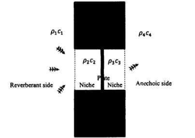
Niche effect depends on some niche parameters such as specimen position in the aperture (Vinokur, 2006). An illustration of the geometry of the problem is given in Figure 2.1. pi,Ci

are the fluid density and sound speed inside the fluid, respectively. The plate is placed inside the niche.

Anechoic side Niche I Niche

Reverberant side

Figure 2.1: Niche and plate configuration. Plate is placed inside the niche.

(24)

2.1.2 Effect of plate location

The effect o f specimen location (Figure 2.2) on STL was considered experimentally by many researchers (Halliwell & Wamock, 1985), (Vinokur, 2006) and (Cops, et al., 1987). Two ways of measurement, sound intensity techniques and conventional techniques are considered by (Halliwell & Wamock, 1985). In their experimental study for each measurement the specimen was placed in five positions inside the niche between two, anechoic and reverberant, rooms and for each position they changed the anechoic room absorption to have four different absorptive conditions. At low frequency range, the STL obtained by the former method is systematically smaller than those obtained by the latter at each position of plate. In both methods the STL was reduced when plate was placed at the center of the tunnel. These results for specimen location are confirmed by (Cops, et al., 1987), experimentally. A possible explanation could be underestimation of transmitted intensity due to the absorption of the panel. The studies of (Kim, et al., 2004) show that the sound transmission, when plate is placed at the center, increases. The difference between STL of plate when it placed at each ends or at center of the niche, is much more noticeable when the depth of tunnel increases. In addition, their findings imply that at low frequencies STL decreases when the panel displaced inside the niche, starting from front-side of the niche to the center and STL increases by shift from center to the back-side of the niche.

Figure 2.2: Three different position of plate inside niche; a) plate placed in front of the niche, b) Plate placed at the center, c) Plate placed in back side o f the niche.

(25)

Schematic results from previous experimental studies (Kim, et al., 2004) (Vinokur, 2006) (Cops, et al., 1987) (Halliwell & Wamock, 1985) is depicted in Figure 2.3. Normalized number to show the plate position inside the niche is defined as:

piate position 2 J

^ length o f niche

where, £ is normalized location of the panel. Figure 2.3 indicates the sound transmission loss of niche in which the plate moves along the niche from reverberant side to anechoic side at a given frequency below the coincidence frequency. The dashed line is STL of finite plate placed in infinite baffle. Previous studies show that sound insulation, in the low-frequencies, is known to be worse for the plate placed at center than either edge of the tunnel. Niche and plate were simulated, analytically, at low frequency by (Vinokur, 2006). He showed that the transmission loss at low frequencies decreases when plate placed at the center of tunnel in comparison to each edge. A ll previous studies, experimental and theoretical, are in agreement with the fact that STL decreases when the specimen is at the center o f the niche, in comparison with situation in which plate is flushed with each side, and this effect is more significant below coincidence frequency.

H on

STL o f niche, plate moves from reverberant side to anechoic side

plate position

0 f _{length o f niche} 1

Figure 2.3: Effect of specimen position, on STL. t, is normalized location of the panel at a given frequency below the coincidence frequency o f the plate

Another experimental study done by (Kim, et al., 2004) shows that the effect o f niche is more noticeable by increasing its length. An effective niche depth means the depth for wich, the

(26)

acoustical behaviour o f the system is affected by niche. The definition o f niche depth is shown in Figure 2.4.

a b c

Figure 2.4: Niche depth definition for three different lengths; L is the depth and d is the depth of reference niche (a); a) normal depth, b) depth is increased, c) depth is decreased.

2.1.3 Effect of niche walls

The influence of the angled baffle on the acoustic radiation o f a flat plate into a semi-infinite domain was studied analytically by (Leppington, 1996). His results indicate that the radiation resistance, with given boundary conditions, is inversely proportional to the wedge angle below the coincidence frequency. Furthermore, analytical expressions are given for the radiation efficiency of edge mode as function of angle baffle. Analytical results o f Leppington were implemented by (Ohlrich & Hugin, 2004) to calculate modal-averaged correction factors. In addition, radiation efficiencies o f isotropic plate were predicted and validated experimentally for different baffle angles, as shown in Figure 2.5. They, in addition, derived analytical expressions for the radiation efficiency of simply supported plate which is coplanar with infinite baffle, in which by knowing ratio of global wave numbers, ratio of acoustic medium wave number over bending wave number, and boundary constraint o f the problem at hand, it is possible to read multiplication correction factor and calculate radiation efficiency of angled baffle.

Excitation

Infinite _Infinite

baffle

(27)

2.1.4 Effect of microphone, loudspeaker, boundary constraints and volume

of rooms on STL

Effects of microphone and loudspeaker position on STL were considered by (Cops, et al., 1987). By using standard deviation for several tests, their findings show that the effects of microphone and loudspeaker position are noticeable at very low frequencies. In addition, for a plate that is placed inside a niche, below coincidence frequencies, STL increases up to 2 dB by placing a reflector plate diametrically in the opening when wave length of sound is smaller than dimension o f the niche.

Having freely hinged edge condition for a plate that is going to be tested is almost impossible practically. So, there is always a difference between experimental results and theoretical ones. To solve this problem (Leppington, et al., 1983) introduced a correction factor for theoretical radiation efficiency formula of plate. They gave the radiation efficiency for edge modes when the boundary condition can be described as hinged with a rotational line-spring that resists the rotation of the plate edge. Hence, by changing the compliance the plate boundary condition can vary from clamped to simply supported edge. The effects of boundary conditions on sound radiation for baffled and unbaffled plates have been studied comprehensively in previous studies (Atalla, et al., 1996); (Xuefeng & Wen, 2010); (Yoo, 2010); (Yufeng & Qibai, 2006). They introduced new approaches for predicting sound radiation from plates with different boundary conditions. In addition their results show that the effects of boundary conditions are noticeable below coincidence frequency; and the radiation efficiency of clamped panel is 3 dB on average higher than free panels.

Results for the shape and size effect of reverberant and anechoic rooms on STL of niche show that equal volume can lead to strong coupling between them. This is the reason of STL decrease under this condition (Cops, et al., 1987). In addition they claimed that their result is valid while the shapes of rooms are equal.

(28)

2.2 Summary

In this chapter, the most important related studies have been reviewed. The most common problem in niche effect studies is repeatability. Significant differences can be seen in the sound transmission loss of the niche when measured in different laboratories. Considering the results of experimental investigation involving the round robin tests, the niche is influenced by not only the system parameters but also the exciting and receiving chambers parameter. These results show that for the same niche system, different STLs from different laboratories are obtained. So, a pure study on niche behavior and the effect o f niche parameters is demanded. Niche effect is introduced as the most important reason for discrepancies between results obtained for systems which includes niche. As shown before there are experimental works on the niche effects and parameter study, in addition there is numerical study on 2D model and 3D model considering the modes of exciting and receiving rooms, but there is no numerical work considering niche parameters independent o f source or receiving room conditions for 3D model.

(29)

CHAPTER 3 SOUND TRANSMISSION LOSS

OF AN APERTURE

3.1 Introduction

Openings can be designed to capture engineering desires such as transferring materials or fluid flow, or they can be consequence of manufacturing or assembly process. When acoustic wavelength is much larger than the size of opening, the latter is known as “leak” while the term “opening” is used for larger dimensions (Sgard, et al., 2007). More recently, a wave based method for aperture coupled to two semi-infinite fluids was proposed by (Sgard, et al., 2007). Here, in the same way of mentioned study, the term “aperture” is used for all dimensions. In this chapter the numerical method which was presented by (Sgard, et al., 2007), to predict the sound transmission loss (STL) o f an aperture with rectangular cross section, is presented. The objectives of this chapter are: first, validate our implementation in FORTRAN of the model with a GAUS written FEM/BEM code (NOVAFEM ). Then, investigate the effect o f aperture thickness and cross section area on STL for both plane wave and diffuse acoustic excitation.

3.2 Theory

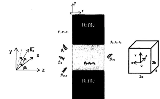
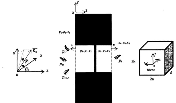
An aperture with a finite thickness and rectangular cross section inserted into a rigid baffle and excited acoustically by oblique plane wave with incidence angles (0 *, <pi) as illustrated in Figure 3.1 is considered. Here 6 is the angle between plane wave and z axis, and <p is the angle between the projection o f acoustic plane wave into x-y plane and x axis, i, is the number of Gauss point in diffuse acoustic filed.

The region is divided into three sub-regions which are; reverberant (sub-region 1), inside aperture (sub-region 2) and receiving (sub-region 3). In Figure 3.1, k Q is the acoustic wave number, {p2>P2*c2} and (P3»P3»c3} are the pressure, density and sound velocity

(30)

p Ris the reflected pressure from interface between medium one and two and pr is the radiated pressure from interface and finally the pr3 is the radiated pressure into medium three by back face of aperture, d is depth of aperture, 2a and 2b are dimensions of aperture in x and

y direction, respectively. And finally, the origin of coordinator “o” is defined at the center of the aperture cross section.

Ha file

htPI.C*

Hal lie

p3ip3'Cl

2a

Figure 3.1: Configuration of the problem; left to right, angles of incident plane wave, pressure definition and coordinate definition.

The total acoustic field in medium one is given by

P i = Pine "b P r "b Pr = Pb "b Pr 3.1

Where, pb is the blocked pressure and convention p (t) = pe;wt is used. As mentioned before the pressure in this medium consists of blocked and radiated pressure. From definition o f block pressure:

p b = A, f = £ ie - i k*xe->kyye - i k*z + § ie - i k*xe - i kyye>k*z 3.2

(31)

where A{ and §j are the incident and reflected pressure amplitude, respectively. kx, ky, kz are the projection of plane wave in x , y and z direction;

k x = k 0 s in 6i cos <pt k y = k 0 s in 6 1 s in 3 . 3 k z = k Q cos di where: (i) k Q = — 3.4 co

Here, o) is the angular frequency and c0 is the speed o f sound in the air. The blocked pressure satisfies the following equation over the interface:

so:

Ki = B t a n d Pb = ^ .e-iko(sinetCos<p1x+sin0i sin<p1y )^ _ jM + 3 6 e - i M + e / M

cos (fc2z) = ---

---Pb = 2Aie -iko(sine,c6s<pfX+sin9lSin<p‘y) (cos(zk0 cos B{)) 3.8

Here z — 0, so:

6 = 2A e_^ko^in0iCOS(,,iX+sin0iSin<|)'y^ 3 9

*0 1

The radiated pressure, in equation 3.1, is calculated using the Rayleigh integral over the surface = S at z = 0. Considering the outward normal vector, H shown in Figure 3.2, the radiated pressure is written as:

(32)

P r(M ) = - J G (M, M0) ( M 0)ds 3.10

on

Batik

n

Figure 3.2: Outward normal vector definition for Rayleigh integral,

where Mand M 0 are two co-planar points at (x , y, 0) and ( x 0, y0,0),

? L = - d- i z 3 .ii

d n d z

and G is the baffled Green function given by:

e - j k 0R

G(M,

W0) =

312

r

= V ( *

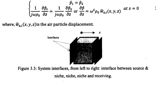
- * „ ) 2 + ( y - y o )2 + U - Zo)2 3 1 3

The studied system consists of two interfaces which are indicated as two separate surfaces in Figure 3.3. According to the coordinate definition, two boundaries w ill be at z = {0, d ).

Where d is the depth of niche. So, from the continuity of pressure and velocity at each interface, the boundary conditions over S = Sls at z — 0 are:

(33)

Pi =P 2

1 d p r 1 d p 2 dp a t z = 0 3.14

o r T “ = W2Po ® a ,i(x >y>z )

;o>p0 dz j o ) p 0 d z d z

where, (S>a i (x, y, z)is the air particle displacement

Interfaces

Figure 3.3: System interfaces, from left to right: interface between source & niche, niche, niche and receiving.

Thanks to boundary conditions and equation 3.10, equations 3.1 is rewritten as following;

d p 2

f 0P2

P i = P2 = P b +

J

G ( M , M 0) ( M 0) d s 3.15

Inside the aperture (in medium two), the state acoustical pressure is governed by the homogenous Helmholtz equation:

V 2p 2( x , y , z ) + ko P2( x , y , z ) = 0 3.16

The acoustic pressure in medium two is approximated in terms o f propagating and evanescent modes, so:

00 00

p2(x ,y ,z) = ^ ^ ( A 2,pqe~iK2p« z + S2pqe,,<2'Pt'z)(ppq(x)y) 3.17

p = 0 q = 0

(34)

^2,pq ~ ^zpq ~ 3.18

*

1 - 0

- ©

f p n ( x + a ) \ f q n ( y + b ) \ <Ppq( x , y ) =

cos I

— J cos f —

J

, p , q = 0,1,2,... 3.19 Substituting in to equation 3.17: £ p q = 0 ( ^ 2,pq "b & 2 ,p q )<P p q (x > y) — P b ~ j E p q = o fs G ( M , ^ o ) ^ - 2 ,p q ( ^ 2 ,p q ~ & 2 ,p q ')(Ppq(.x 0> y o ) d s

By multiplying by <puv (x , y ) and integrating over S:

00

£

f ' ( P u v ( x ,y ) ( A 2lpq + ^2,pq)<Ppq( x , y ) ds

= I

<Puv(.x,y)pbds *S CO j

^

f J <Puv(x, y )G (M > M q ) k2ipq ( A 2 pq p q = 0 5 5

-

^2fiq)<Ppq(x0, y 0) dsds 3.20 p q= 0 s 3.21

In order to simplify the equation 3.21, definitions of norm, N pq, exciting field, Pp q , and

aperture cross modal radiation impedance, t uvvq, are introduced in equations 3.22, 3.23 and 3.24, respectively; Npq = f (ppq ( x , y ) d s 3.22 Js Ppq = [ <Ppq(x,y)pbds 3.23 ■'s j Z K f f %uvpq ~ ~

- J

J < P u v ( x ,y ) G ( M ,M 0)<ppq( x 0 ly 0) dsds 3.24 18

(35)

Here 2 uvpq is the aperture cross modal radiation impedance between modes (u, v) and (p, q )

and Z 0 and K0 are the characteristic impedance and wavenumber of air, respectively. For a rectangular cross section and it is given by:

2

*'uvpq

JJsr /- «& /- « /-b

cos ( lr ) cos (

1

?)

G(-Xi y>

cos Gl?)cos Olr)

dy0d x 0dydx

The quadruple integral, equation 3.24 is change into double integral and is solved via the Gauss quadrature method (Nelisse, et al., 1997); for more details see Appendix B. So, equation 3.21 can be rewritten as:

00

(^2,pq + &2,pq)Nuv6UVpq — Ppq , / ^2,pq{.^2,pq &2,pq) ^uvpq 3.26

Z0K0 Z—Jn _{p q}_{= 0}

For back side of the apertures, medium three, the radiated pressure is obtained by implementing the Rayleigh integral over the backside surface:

f dp? d p3 d p3

p3(M ) =

-J

G ( M , M 0) j ^ ( M 0) d s 2 a n d j ^ = - ^ 3.27 The boundary conditions over S = S2 at z = d are:

A A

P2 = P3

1 d p2 1 d p3 d p _ 2 A , Na t z = d 3.28

jo ip o d z j(i>p0 d z d z

Using these boundary conditions and equation 3.27:

P3 = P 2 = - J s G ( M , M 0) ^ ( M 0) d s 3.29

(36)

p q = o

( A 2iPqe ~ JK2'P<id + B 2pqe jK2P‘i d)(ppq( x , y )

00

= j Y , { k 2.P d(A 2,Pqe ~ JK 2pqd

3.30

pti=o s

- B 2>pqe iK2P<id)(ppq{ x Q,yQ) G ( M , M o ) d s

and multiplying to <puv (x , y), integrating over 5:

VM

J <Puv(x,y)(A2iPqe~JK2^ d + B2pqe iK2^ d)(ppq( x , y ) ds

p q=o 5 uu = i X / / p q = 0 s s - § 2,pqe jK2P«d)<ppq( x , y ) G ( M , M 0)d s d s 3.31

Using the definition of norm and cross modal radiation impedance, equation 3.31 is rephrased as: ( A 2 , p q e ~ j l < 2 ' P q d + B 2 p q e i K 2 ^ d ) N i v 8 ,uvpq z 0k Q uo k 2iPq ( A 2'Pq e - j K 2 P < d - B 2tVqe i K 2 P«d ) I 3.32 uvpq p q = o

Equations 3.26 and 3.32 are cast in matrix format to calculate the unknown vectors, A 2 iP q and

®2,pq-ft

_{6 1} '[A2,pq]}

*3

W

m , Pq]\

I [

₀

] J

3.33

where, {ft} are sub-matrices defined as follows:

(37)

00 5 $ 3 , u v p q ~ e ^ K z p q d N u v ^ u v p q ^ f t ^2, p q ^ u v p q e ^ 2 p q 3.36 ° °P<?=0 00 f . = p i K2.pq d N 2 A -|_________ > f p i K2,pq d 'I 1 7 *>4,uvpq e l'uv°uvpq % K 2 - j 2’PQ UVPQ •5"5'

The rank of general matrix, and sub matrices are defined in the following:

h = 4 x (pma* + 1) x (qma* + 1) 3.38

where {pmax, Qmax} are the maximum number o f kept mode in {x, y } direction for niche.

3.2.1 Calculation of vibro-acoustic indicators

Thanks to Prof. Sgard’s subroutines, the equation 3.33 is implemented in a FORTRAN code and solved for a given incident oblique plane wave and diffuse acoustic field, using the linear algebra package “LAPACK”. The output o f the solver is two unknown vectors, A 2iPq and

B 2 lp q , which are coefficients of pressure distribution inside the aperture, equation 3.17.

Transmitted acoustic power for one oblique plane wave is calculated as follows:

nt

(fii.vd =

J Re [js p3u|,„(is] =

B 2 .p q e * K2,pqd)<Ppq(.x > y ) Emn=0 % 2,mn(“ ^2,mne_^ 2'mn * + B2,mne]K^ ndy<Pmn(x,y ) ds] = \R e g DpqN*q K 2,pq£*pq]

3.39

(38)

D p q = A 2 m e ~ > K w d + 8 2 ,p q e j K w d

P p q = - A 2 , v q e ~ i H p q d + K p q e i H p q d

3.40 3.41

The incidence power is given by (Fahy & Gardonio, 2007):

|i4jl2 cosfl(S

n l n c ( 6 i . < P i ) = ₂_p0C0 3.42

Whit respect to power incident and transmitted power, the oblique incidence transmission coefficient, t(0 {, <pi) is calculated:

rit (9(, (pi)

3.43

3.44 nine (^i> 'Pi)

Finally the STL can be calculated as:

STL = - 1 0 log t

3.2.2 Transmitted power for diffuse acoustic field

Since there are more than one plane wave in diffuse acoustic field, the unknown coefficient vectors and exciting force sub-matrices are changed as follows:

$ 2 A 2 ,pq •" n 2,pqA ' U s w h x h A,p<? ■• P '2 .p q . _{h x k}

= { ]

PQ 0 P tv j)_pq o h x k 3.45

where h is defined in equation 3.38 and k is:

k = n u m b e r o f Gauss p o in t s a cro s s 6

x n u m b e r o f Gauss p o in t s ac ro ss <p

3.46

Here, A ' 2 p q , P ’ z iP q are unknowns associated to i t h plane wave and P ' p q is the exciting force

associated from that plane wave. Plane wave Transmission coefficient is calculated as following:

(39)

Td i f f ~

Jo *

I o Um r (e t>

<Pi) sin

6 i

cos

di d6d<P

3.47

7r s i n 2 ^ i im

where r(fy, (p{) is the transmission coefficient for each plane wave and

3.48

The transmission loss is calculated as following.

STL = - 1 0 lo g t 3.49

3.3 Numerical examples

In order to validate the proposed model and FORTRAN code, several examples are considered, the results are compared with NOVAFEM. The convergence of acoustic indicators, sound transmission loss and radiation efficiency, has been studied by looking at discrepancies as the number o f modes increases. First, the convergence of the proposed model is investigated by focusing on transmission loss and on truncation frequency which is directly related to the number of modes kept in the modal expansion. Second, results are compared with results obtained by hybrid finite element method-boundary element method (FEM-BEM) for different excitation types.

3.3.1 Convergence of the approach

Aperture dimensions, fluid density and speed of sound inside the fluid and frequency interval are given in Table 3.1.

Table 3.1: Characteristics of aperture

2a x 2b x d (m) pn (kg/m3~) Cn (m /s) Frequency range (Hz) 0.4 x 0.2 X 0.05 1.213 342.2 10- 2000

(40)

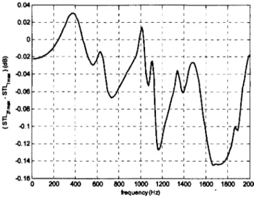
As mentioned before, the number of modes plays important role in presented method. So, the effect of number o f modes on sound STL is studied. Excitation parameters for both plane wave and diffuse field are detailed in Table 3.2.

Table 3.2: Excitation field characteristics

Pressure amp. F r e q u e n t Plane wave Diffuse acoustic field

Ai (pa) fmin” fmax(Hz) e _<P Number of Gauss points in 0 Num ber of Gauss points in <p Ollm

1 1 0 - 2 0 0 0 45* 6 0 ' 2 0 20 78*

The STL difference between two truncation frequencies, f max and 2f max, is shown in Figure 3.4. Keeping modes up to the maximum frequency is good enough to capture the physics of the problem. The maximum difference between these two solutions is less than 0.16 dB for the frequency range and plane wave excitation. So, with respect to this result and minimum acoustic wave length and lateral size of the aperture, in this chapter, modes up to

f max w ill be retained in the modal expansion.

0.04 0.02 sr -0.02 " , *0.04 ■0.08 -0.1 -0.12 -0.14 -0.18 frequency (Hz)

Figure 3.4: Convergence study, the effect o f keeping modes up to two times of truncation frequency.

(41)

3.4 Numerical validation

In this section the results obtained from presented method are validated by the results obtained by NOVAFEM. The aperture is modeled in FEMAP as shown in Figure 3.3. The aperture volume is discretized using acoustic brick (Hexa 8) elements. Coupling with the source and receiver semi-infinite fluid is taken into account with a Rayleigh integral based impedance radiation matrix implemented within NOVAFEM (Sgard, et al., 2007). Since the convergence is slow (see Figure 4.7), 10 elements per acoustic wave length, Xa is considered here. Number o f the elements in each direction is given in Table 3.3.

Table 3.3: Number of elements for the aperture modeled in NOVAFEM

Direction 2a 2b d

Number of Elements 30 20 4

K = ~ r ~ * 0.18 (m ) 3.50

Jmax

Two examples are considered here; the first, system is excited by a normal incident plane wave. Sound transmission loss o f the system obtained by FEM -BEM method through NOVAFEM and proposed method is shown in Figure 3.5. In this figure a eq is ^ j A a b / n. The second, the STL of the aperture excited by an oblique incidence plane wave with the parameters mentioned in Table 3.2 is shown in Figure 3.6 .

(42)

— NOVAFEM e F. Sgard Mathod

t

to

Figure 3.5: Comparison of presented method and FEM-BEM. Normal incident (0* = 0°

,<Pi

= 0°) transmission loss o f rectangular aperture (b/a=l/2, d/a=l).

I fi

V)

Figure 3.6: Comparison of presented method and FEM-BEM. Oblique incident (0£ = 4 5 °, <Pi = 60°) transmission loss of rectangular aperture (b/a=l/2, d/a=l).

As shown in these figures, there is an excellent agreement between the proposed approach and FEM-BEM model. The effect of aperture length on STL w ill be studied in next section by using the proposed method.

(43)

3.5 Aperture depth and shape effect on STL

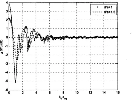
Effect of aperture depth on STL for two kinds o f excitations, oblique plane wave and diffuse acoustic filed as explained in Table 3.2, is investigated here. The ratio o f cross section dimensions is b/a=0.5. Several ratios of aperture depth to larger dimension, a, are considered as d/a= 0.25, d/a = 0.5, d/a = 1 and finally d/a=1.5. The results are given in Figure 3.7 for the plane wave case and in Figure 3.8 for the diffuse acoustic field. It is observed that the aperture effect is considerable up to ( k 0 a eq = 4 ). The effect o f aperture is negligible (S TL < 1 d B )

where k 0 a eq > 4. The transmission loss at high frequencies converges to 0 dB which means the aperture effect vanishes when acoustic wavelength becomes smaller than niche length while at low frequencies it increases as the aperture length is increased. It means that the transmission coefficient is 1 at high frequencies; in the other words, the aperture effect vanishes when the acoustic wave length is small enough to neglect the diffraction effect.

For apertures with larger depth, d/a > 0.5, the transmission loss shows resonant behaviour. In addition, by doubling the depth ratio, d/a, STL increases about 2 dB before the first transverse mode for both type of excitations, plane wave or diffuse acoustic field. This means increasing the length up to two times w ill cause 60% reduction in transmitted power caused by first mode. Effect o f increasing the depth up to two and three times o f d/a=0.5 is shown in Figure 3.9.

Effect of excitation field, diffuse or plane wave, is shown in Figure 3.10 for two apertures with different depth. As shown in this figure the effect of diffuse field, Table 3.2, is less than 1 dB for all frequency range. The same result is obtained when the depth increase up to two times. The STL difference for both cases is less than 1 dB for all frequency range.

(44)

d/a=0.25 - d/a=0.5 — d/a=1 d/a=1.5 S_2, k a₀

Figure 3.7: Effect o f niche-depth on STL under plane wave excitation field.

d/a=0.25 d/a=0.5 d/a=1 d/a=1.5

K a_{0 aq}

Figure 3.8: Effect of niche-depth on STL under DAF excitation field.

(45)

i

' '

_I

_i

i

d/a=1

it

1

i

i 1

I

i

d/a=1.5

^

- r -

n

Si ."'P !w

jl?

i

•<? !«r s

lifoti ’

i

1 !

- 1-pjO +

1 f ■

i f

;

1 :

1

1 I; ■

1 _t!

1

1 **I* 1**

’j

- Sf t

-1

1

1 i

1

1 5 r

t

i

1

1 I

i

i... L... ... J... . _1_____

Figure 3.9: Effect o f increasing the depth up to two and three times under plane wave excitation. The reference system depth is d/a=0.5.

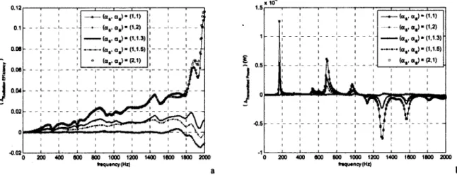
0.8 d/a-0.5 •B — d/a=1 0.7 0.6 m S. 1 0.5 i 5 0.4 0 £ 0.3 1 0.2 £ ■0.1

Un modele vibroacoustique pour prevoir l’effet de niche sur la perte par transmission sonore