HAL Id: hal-02615395
https://hal.inria.fr/hal-02615395
Submitted on 22 May 2020
HAL is a multi-disciplinary open access
archive for the deposit and dissemination of
sci-entific research documents, whether they are
pub-lished or not. The documents may come from
teaching and research institutions in France or
abroad, or from public or private research centers.
L’archive ouverte pluridisciplinaire HAL, est
destinée au dépôt et à la diffusion de documents
scientifiques de niveau recherche, publiés ou non,
émanant des établissements d’enseignement et de
recherche français ou étrangers, des laboratoires
publics ou privés.
Chemoinformatics approaches to help antibacterial
discovery
Clément Bellanger, Jane Hung, Nyoman Juniarta, Vincent Leroux, Bernard
Maigret, Amedeo Napoli
To cite this version:
Clément Bellanger, Jane Hung, Nyoman Juniarta, Vincent Leroux, Bernard Maigret, et al..
Chemoin-formatics approaches to help antibacterial discovery. [Technical Report] Inria Nancy - Grand Est.
2020. �hal-02615395�
Chemoinformatics approaches to help antibacterial discovery
Clément Bellanger
∗, Jane Hung
§, Nyoman Juniarta
∗, Vincent Leroux
∗, Bernard Maigret
∗, Amedeo
Napoli
∗∗Université de Lorraine, CNRS, Inria, LORIA. F-54000, Nancy, France
§Broad Institute, Harvard / Massachusetts Institute of Technology. 02142 Cambridge, USA corresponding author email: [email protected]
ABSTRACT
Many bacteria are acquiring more resistance to usual treatments worldwide, to the point that the possible advent of pathogens resis-tant to the entire current arsenal is a true concern. Therefore, there is an urgent need for finding new effective antibacterial drugs. As-sociated to data mining methods, in silico ligand-based drug design techniques may extract the most relevant molecular features and eventually lead to the discovery of innovative potent antibacterial molecules. In this work, we use feature selection techniques to build molecular filters with demonstrated ability to discriminate between antibacterial and non-antibacterial small molecules. A very large number of molecular properties translated into molecular descrip-tors, being simultaneously diverse and redundant, were processed using various feature selection techniques.
It is shown that this approach was efficient in decreasing the models complexity by identifying most relevant features for antibac-terial activity. For reducing the number of considered descriptors, we have trained multiple machine learning algorithms until result-ing models performance in virtual screenresult-ing could not be optimized further. We also discuss the interest of using log-linear analysis to improve our data-driven process and to increase the chance to predict efficiently new antibacterials.
1
INTRODUCTION
Bacterial and parasitic diseases are the second leading cause of death worldwide, according to reports on antibiotic research released re-cently [5, 25, 34]. Currently, a pressing public health concern origi-nates from bacterial resistance to the available arsenal of antibiotics. This natural phenomenon is occurring more and more frequently, probably due to evolutionary pressure fueled by mis-use/over-use of current drugs. The emergence of “superbugs” resistant to en-tire antibiotic classes may render traditional antibiotics obsolete in the coming years, with potentially dramatic consequences [25]. Consequently, new antibiotics are desperately needed, preferably featuring novel mechanisms of action in order to successfully fight multidrug-resistant strains [12, 14, 27].
Unfortunately, the amount of money being spent in antibiotics R&D is woefully inadequate as major pharmaceutical companies mostly focus on different pathologies according to their pipelines. Drugs against chronic diseases highly common in modern devel-oped countries (e.g cardiovascular deficiencies, diabetes, obesity) certainly promise higher and faster returns to the shareholders, yet there are certainly a lot of profits to be potentially made with antibiotics. For instance, once the death toll for hospital-acquired in-fections of multidrug-resistant strains of the likes of Staphylococcus aureus become unacceptable (and that will happen too soon if no
progress is made), a new efficient antibiotic class could eventually turn out to be the only option to save lives.
In this context, in order to make progress in this field, resorting to more modern techniques, even if those have not demonstrated sim-ilar success rates so far in classical drug discovery programs, looks like a rational choice. Computer-aided techniques have already proven their usefulness to save time and money in the drug discov-ery process [39]. In particular, ligand-based drug design calculations (i.e. QSAR) are now well-recognized as fast and efficient approaches in the hit-to-lead early drug discovery phase. Knowledge discovery approaches (e.g machine learning, data mining, neural networks) are less mature in the context of drug design but their success in other applied computing fields make them increasingly promising. They are also especially popular in academia since provided they are combined with very strong interdisciplinary expertise; they may allow overcoming the lack of experimental data useful for medicinal chemistry projects compared to what is existing in the industry. Furthermore, one hope is that progress in the chemoin-formatics field [4] could eventually allow finding possible “hidden gems” amongst the millions of available chemicals from providers, companies or laboratory collections, and even established drugs.
Here, we present an in silico strategy targeting antibacterial molecules identification in a virtual screening context. Our final goal is to be able to highlight molecules within existing chemical collections with a high probability of being potential antibacterials and that could not be found using most of the existing similar approaches.
Considering the huge variety of molecular descriptors that can be used [43] in order to describe molecular properties, the prob-lem is how to achieve an optimal selection of molecular attribute sets in order to analyze, with highest accuracy, chemical diver-sity/similarity among large (>1M objects) chemical libraries. Such “optimally-selected descriptors” should provide the most efficient rules which can be used next to describe molecules with a com-mon behavior, in this case antibacterial potency. Dimensionality reduction in the descriptors space has already been considered as an important issue in QSAR methods [19, 22, 24, 35, 38]. The knowl-edge discovery phase would then next allow to extract, among large chemical datasets, compounds presenting all the same required ac-tion.
2
DESCRIPTION SPACE REDUCTION AND
TRAINING PROCESSES
In this section, we apply and compare several well-established machine learning algorithms against the same training datasets appropriate for the problem of antibacterial molecules identification.
It is demonstrated that the resulting filters are efficient, and those will serve as references to evaluate future new knowledge extraction methods we are currently investigating.
2.1
Methods
2.1.1 Molecular data sets. In order to train feature selection tech-niques for discriminating antibacterials and non-antibacterials, we built several molecular training sets of both antibacterial and non-antibacterial molecules from different sources.
• Set P1 (positive) is constituted by 150 antibacterials that are part of the current standards of care in France [44]. • Set P2 is the antibacterials subset of the MDDR 2016
data-base [3]. It comprises 2854 molecules annotated as possessing antibacterial potency and not already referenced in the P1 set.
• Set P3 is the Life Chemicals [1] supplier’s antibacterial library. As retrieved for this study, it contains 38907 small-molecule, drug-like compounds available for purchase, that have been selected from the full supplier catalog using proprietary clas-sifiers.
• Sets N1 (negative), N2, N3 and N4 are built from MDDR molecules that are not tagged as antibacterials but having completely different known activities. N1 has 1519 analgesic compounds, N2 has 3654 compounds targeted at cardiovas-cular diseases, N3 comprises 17796 compounds marked as “antagonist” and N4 34210 marked as “inhibitor”.
• Set N5 is an ensemble of Life Chemicals molecules available for purchase not found in P2 nor in N1–N4. It comprises 52604 molecules from the cancer-, central nervous system-and analgesic-focused libraries.
To focus our study on small molecules, all molecules in our data sets were imposed to have molecular weight less than 600 Daltons. A single 3D conformation of all these compounds was obtained from Corina [36].
2.1.2 Attribute sets. For each molecule, a set of 4885 attributes were calculated from the Dragon software [19] describing constitutional, topological and geometrical properties. While molecular descriptors calculations are available in several QSAR platforms [2], Dragon combines a particularly large choice and diversity with a clear and detailed technical documentation. Attributes where values were missing were removed. Some of the attributes were found perfectly correlated; in such cases we removed all but one attribute from each group. This resulted in a baseline number of 4532 attributes. Models were run on data sets with 5 different attribute sets that will be referred to as F0, F1, F2, F3 and F4 next. F0 contains the baseline 4532 attributes while F1–F4 have filters applied in order to limit the number of attributes; such restrictions may positively impact the final classifier performance. All filters are based on thresholds about computed values. F1 eliminates attributes that result in a data distribution with standard deviation σ < 0.01 and with pair correlation ρ ≥ 0.4. F2 excludes σ < 0.01 and ρ ≥ 8. F3 excludes σ < 0.001 and ρ ≥ 8. F4 excludes σ < 0.1 and ρ ≥ 8. 2.1.3 Classification algorithms. We applied the following popular classification techniques: support vector machines (SVM) [11] with linear kernel, random forest (RF) [6], logistic regression (LR) [40],
gradient boosted trees (GBT) [16], naive Bayes (NB) [26], and de-cision trees (DT) [26]. Besides predicting classes, most of these methods output a measure for feature importance that can be used to infer relationships between specific molecular properties and ac-tivity (here: identification as antibacterial). All classifications were implemented in Python language using Scikit-learn [7, 28]. SVM was implemented using the LIBSVM package [10] with a linear ker-nel. For SVM and LR, the testing data was normalized based on the training data, regularization parameter C was varied by factors of 10 from 10−6to 10. Regularization is a process of introducing extra terms to reduce overfitting by discouraging complexity. For RF and GBT, 1000 estimators were used because there was no significant improvement using more. Tuning the C parameter was found to improve performance (as measured by precision) so by averaging the results of the first step for each value of C. The best performing C was chosen for each data set.
2.1.4 Training process methological details. Different scoring meth-ods like precision (probability of a positively classified element being positive), recall (probability of a positive element being posi-tively classified), accuracy (probability of a correct classification), f 1scor e(harmonic mean of precision and recall) and AUC (area
under the ROC curve) were calculated. The most relevant score for our purposes and our main metric is precision because we want a high probability of our predicted antibacterial molecules being true antibacterial molecules. For screens involving a large number of molecules, of which only a few are to be chosen for closer study, it is important to choose compounds with the maximum likelihood of being antibacterial. However, recall must be high enough to obtain enough molecules to test. When looking for new potential antibac-terial molecules, it is very important that after classification we obtain a list of molecules that is reliable rather than a more ambigu-ous list containing both more antibacterials and non-antibacterials. ANOVA and Tukey’s Honest Significant Difference (HSD) were used to identify which means were significantly different (with significance for p < 0.05).
At each phase of the validation/optimization process, different independent runs are done. A discriminating parameter α was therefore introduced to derive the molecule final classification, which may not be consistent. The α is defined as follows: a molecule is being considered antibacterial if it was classified as such in at least α % of the runs.
2.2
Results and discussion
2.2.1 Summary of starting datasets. As explained in Section 2.1.1, the molecules were collected from market, MDDR, and Life Chemi-cals. This set of molecules is illustrated in Figure 1.
From those molecules, five data sets are constructed. Each of them has the same set of molecules, but different attributes, ac-cording to standard deviation and pair correlation explained in Section 2.1.2. The resulting number of attributes on each data set is detailed in Table 1.
2.2.2 Training and testing strategy. Three distinct training/testing stages were implemented:
(1) Our first step was to evaluate all classifiers performance. For that, we trained all methods (SVM, LR, RF, GBT, DT, NB)
Figure 1: Diagram showing the intersections between molecules from market, MDDR, and Life Chemicals.
Table 1: Rules and number of attributes of each filter
Filter Stddev Pair correlation Selected attributes 1 ≥ 0.010 < 0.4 87 2 ≥ 0.010 < 0.8 576 3 ≥ 0.001 < 0.8 588 4 ≥ 0.100 < 0.8 524
against the on-market antibacterials set P1 as the positive set and Life Chemicals non-antibacterials N5 as the negative set. Because the non-antibacterial class is over-represented, we randomly undersampled this class to do cross validation. Therefore, a random set of 150 N5 molecules was generated. Next, 100 random P1 and N5 molecules were used for training and the remaining 100 (50 in each set) formed a test set. This process was repeated 50 times. The aim of this first stage is to allow the identification of the most appropriate attribute set and filter out the least interesting classifiers.
(2) Next, the three top-performing classifiers from the first stage are retained and applied to an independent set of data. The F0 descriptor set (4532 unfiltered attributes) is trained against P1 and a set of 150 random N5 molecules, then the resulting clas-sifier tested on an ensemble composed of P2, N1, N2, N3 and N4 (all from the MDDR database) assuming all P2 molecules are actual antibacterials and that there is no antibacterial in N1, N2, N3 and N4. This training process is repeated 10 times and the number of times each molecule was classified as non-antibacterial and antibacterial was recorded. Then we calculated the total combined precision and recall with the antibacterial being the positive class. Because there were 10 runs, we decided on molecules’ “final” classification by using the α parameter defined before.
(3) For our third step, we applied the models from the second step to the P1 and N4 MDDR set. We trained the classifier on the 2854 P2 MDDR antibacterials and 2854 randomly chosen MDDR N1, N2, N3. The training was repeated 10
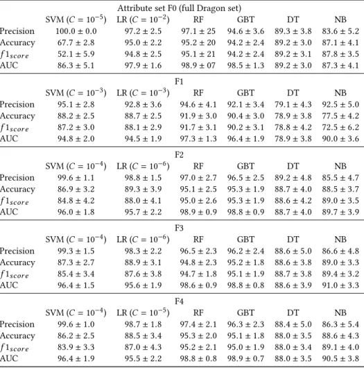
times and the number of times each molecule was classified as non-antibacterial and antibacterial was recorded. 2.2.3 Attribute set comparison and initial classifier evaluation. In the first step described above, we have tested all classifiers against all attribute sets. The results are summarized in Table 7.
All classifiers perform better than chance regarding our main metric precision. SVM, LR, RF, and GBT have better precision than NB and DT across the 5 different attribute sets. SVM appears to be the best performer with respect to our main metric precision for all data sets, though it is not significantly different from RF for attribute set F1 and from LR for F2 and F3. Over 99% precision is reached with SVM for all sets except F1, but it suffers from lower accuracy and recall, meaning it only correctly classifies a small percentage of antibacterials but those that are classified as antibacterial are correct. This can be seen most clearly in the F0 case, where accuracy and f 1scor e are 67.7% and 52.1%, respectively, compared to > 90% for
LR, RF, and GBT; the relatively low accuracy and f 1scor e, as well as
low training accuracy (68.2%) and f 1scor e(53.2%), are indications
of under-fitting by this model.
The precision results with F2, F3, and F4 are comparable to F0. In particular, the SVM precision with F0, F2, F3, and F4 is not sig-nificantly different, but the accuracy, f 1scor e, and AUC are worse
with F0. The improved performance of some of the classifiers with reduced attribute sets may be due to some sensitivity to highly-correlated attributes or over-fitting to irrelevant attributes. F1 still results in > 90% precision for SVM, LR, RF, GBT, but the results are significantly worse than with F0, F2, F3, and F4, probably because important attributes were eliminated by the low correlation thresh-old. Definitions for F2, F3, and F4 do not result in such a problem, since metric scores are similar for all classifiers.
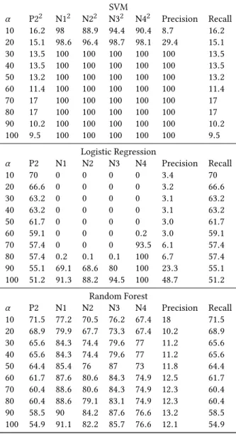
2.2.4 Final classifier selection. In our final step, we took the best performing models–SVM, LR, and RF–trained on the P1 and N5 sets to test the MDDR data. Separately testing on the MDDR P2 antibacterials and non-antibacterials (i.e. N1 analgesic, N2 cardio-vascular, N3 antagonist, N4 inhibitor), we calculated the propor-tion of molecules correctly classified where molecules classified as antibacterial in at least α percent of runs were classified as an-tibacterial; for each classifier, we also combined the MDDR data and calculated the precision and recall with respect to antibacterial where a molecule was classified as antibacterial if it was (Table 8). A low value of α (less than 50%) can be used if we want a permissive definition of antibacterial, but generally we are most interested in values above 50%.
Similar to previous results, SVM shows higher precision but lower recall. The MDDR non-antibacterials (N1-N4) have high per-centage of correct classifications for all α values while less than 20% of MDDR antibacterials are classified correctly. Despite this, because the proportion of non-antibacterials compared to antibac-terials is 20:1, precision ranges from 8% to 100% while recall stays below 20%. SVM with moderate α may be used as a model that out-puts a small list of molecules that are very likely to be antibacterials; however, this list could also be too small for efficient experimental testing.
LR shows very erratic results with varying α . For low α values, most antibacterials in the test set are retrieved, while for high α (less stringent screening), most non-antibacterials are correctly
found. Around α= 80%, the non-antibacterials show a steep rise in proportion of correct classifications and precision jumps from 6% to 23%, achieving a maximum of 48%. Most non-antibacterials were classified as antibacterial between 1 and 7 times out of 10 runs. This inconsistency makes LR an untrustworthy model for our purposes. As expected from an ensemble model, RF shows more consistent results. Precision stays around 10-12%, which is far smaller than the highest precisions achieved by SVM and LR. Although RF classifies most non-antibacterials as such, a large number of them are false positives compared to the number of true positives. RF’s recall is much better than SVM, so RF could be used as an alternative in case it is worth sacrificing the precision of SVM for higher recall. To maximize precision, we choose SVM for the last training stage.
3
KNOWLEDGE DISCOVERY WITH
DECOMPOSABLE MODELS
In Section 2, we inspected a number of chemical molecules to know which features could characterize antibacterials. To do that, we used the properties of each molecule, summing up to thousands of molecular attributes providing a significant amount of data to be analyzed for knowledge discovery.
In order to minimize the required time and space, before we mine the data, we should reduce the dimension of the data set, as a transformation step according to the basic steps of KDD [13]. It is performed by combining some attributes into one, or by completely eliminating some of them.
Within the thousands attributes for each molecule, we can iden-tify some redundancies and therefore, we can ignore an attribute if it can be merged or replaced with another attribute. The selected attributes should be able to define the molecules without significant loss of information. Beside the redundancies, we should also ignore the attributes which are not informative.
3.1
Log-linear analysis
Log-linear analysis (LLA) can find any associations among attributes, allowing feature selection according to those associations.
Suppose that we have a data set W AR of certain molecules with three variables: molecular weight (W ), number of atoms (A) and ring perimeter (R). Relationship between two variables can be studied with two-way χ2test of association. However, if we have more than two variables, we need to do a multiway frequency analysis to study the two- and three-way associations. LLA is an extension of multiway frequency analysis, and tries to discover any statistical relationships between three or more non-continuous variables. It will create a model (like the one in Eq. 1) to find the log of expected frequencies.
For the W AR, LLA tries to answer some relationship questions. Is a molecule’s weight related to its number of atoms? Is a molecule’s number of atoms related to its ring perimeter? Is there a three-way relationship among molecular weight, number of atoms, and ring perimeter? By knowing ring perimeter of a molecule, can we predict its weight?
To do a multiway frequency analysis with LLA, we develop a lin-ear model of the logarithm of expected cell frequencies. An example of such model is shown in Eq. 1, with each term representing an
association. As the number of variables increases, the number of as-sociations also increases. With three variables in data set W AR, we have seven possible associations: one three-way associations, three two-way associations, and three one-way associations. The model in Eq. 1 contains all possible associations. To keep the simplicity of a model, LLA tries to find which association will be kept or removed. To do that, we should determine the significance of an association by examining the goodness-of-fit of the model containing it.
Eventually, with thousands of variables, the number of possible associations will be so large that it would be impractical to test each association. This limitation can be solved by Chordalysis. 3.1.1 Log-linear model. Log-linear model is represented as an equa-tion to find a logarithm of E (expected frequency of a combinaequa-tion of variables’ values). From data set WAR, we can generate a model that contains all possible associations. This is the saturated model, which can be written as:
ln Ew ar = θ + λW(w)+ λA(a)+ λR(r )
+ λW A(wa)+ λW R(wr )+ λAR(ar )
+ λW AR(war ) (1)
where θ is a constant, and λ term represents an effect. Each λ has values as many as the number of levels, and these values sum to zero. For example, since we define three levels of molecular weight: light, medium, and heavy, λW(w) has three possible non-zero values:
for light (λW(lig)), medium (λW(med)), and heavy (λW(hvy)), with
λW(lig)+ λW(med)+ λW(hvy)= 0.
A log-linear model can be hierarchical or non-hierarchical. A hierarchical model can be represented by its highest-order associ-ation in square brackets. For example, a model [W A][R] contains λW A(wa) and λR(r ), as well as λW(w) and λA(a).
Furthermore, if a model is a sub-model of another, their G2 differ-ence is itself a G2. Therefore, [W A][R] is a sub-model of [W A][W R], i.e. we can find all λ terms of [W A][R] in [W A][W R]. By comparing their G2to χ2table, we can obtain their significance. If both models are significant, we can choose the less complex one ([W A][R]) if their G2difference is not significant.
3.2
Chordalysis
There are two ways to select which associations to include in a log-linear model, backward elimination and forward selection. Back-ward elimination starts from a saturated model and eliminates non-significant associations one by one. On the other hand, for-ward selection starts from an empty model and iteratively adds an association until the difference is not significant. The existing LLA considers all possible associations to determine which one to be added or removed. This becomes infeasible when the number of attributes increases, since the number of associations is exponential w.r.t. it.
Chordalysis tries to guide the existing LLA in selecting which associations are significant enough to be included in the model [30, 32]. This method is focusing on decomposable log-linear models, whose G2can be calculated by inspecting the maximal cliques and minimal separators of the corresponding graph.
As a forward approach, Chordalysis starts with an empty graph as initial model. It has neither vertex nor edges. Then at the first
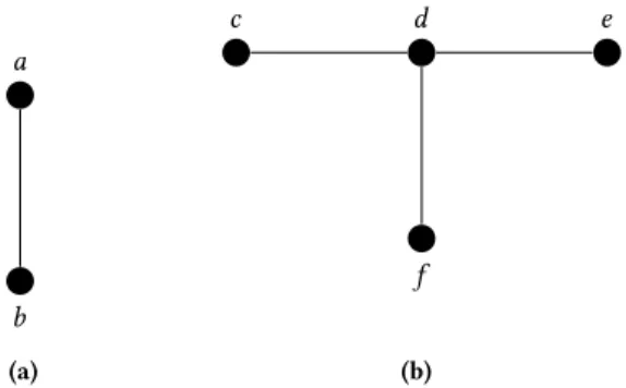
a b (a) c d f e (b)
Figure 2: Examples of connected components with 2 vertices (a) and more than 2 vertices (b).
step of each iteration, the candidate models are generated. Each can-didate Mcdiffers from the current best model M∗by a single edge only. Therefore, we try to add an edge at each iteration. This edge addition must keep the graph chordal, hence the name Chordalysis. Based on the fact that the graph is chordal and differs by an edge between iterations, the G2 computation is scalable to thousand variables [31].
After the score calculations, Chordalysis selects the best Mc. Its score is then compared to the significance threshold. If it is lower, then we replace M∗with Mcand continue to the next iteration. If not, then the current M∗is the final model because the G2difference by adding an association is not significant.
The significance threshold α is updated at each iteration so it does not accept a candidate too often. This update rule follows the layered critical values [46]. At iteration i, where the current best model M∗has L edges, the significance threshold αi is:
αi = α
2L· S i
(2) where Si is the search space, i.e. the number of chordal graphs that
can be formed by adding a single edge to M∗, and α is a p-value threshold (usually set to 0.05).
Having a graph representing associations among attributes, we then perform feature selection based on this graph. The attributes which are independent (have no association) are kept, because they can’t be represented by another attribute. Then, basically we remove the attributes that have only one association. For example, if we encounter a connected component shown in Fig. 2b we keep only attribute d. This means that d can represent c, e, and f . But there is an exception for some of those one-association attributes. If a connected component has only 2 vertices, like the one in Fig. 2a, we randomly choose one attribute and discard the other.
3.3
Classification of antibacterials and
non-antibacterials
The attributes that are selected using Chordalysis will be used in three machine learning method to classify dataset of antibacterials and non-antibacterials.
The first method is Support Vector Machine (SVM) [11]. Given a dataset of labelled points, SVM builds a hyperplane that best
separates the two labels. To deal with non-linearly separable dataset, SVM use a kernel to map points to higher dimension.
The second method is random forest [6]. It constructs a family of decision trees which have different training set between each other. To classify data, each tree gives a classification (or “vote”), and random forest takes the majority vote.
The third method is naive Bayes [26] that is based on Bayes’ theorem. When classifying a data d, naive Bayes calculates the pos-terior probability of each class given d. The classifier then chooses the class that has higher posterior probability.
3.4
Result
To measure the goodness of each classifier, we use five metrics: accuracy, precision, recall, AUC, and f 1scor e.
Here we focus on 3025 antibacterial molecules, which is com-posed by 152 molecules from market and 2873 molecules from MDDR antibacterials. From those molecules, we defined 4885 at-tributes. Besides removing missing-valued attributes and perfectly correlated attributes (like the previous work in Section 2), we also removed attributes that have the same value for all molecules. This resulted in 3769 attributes.
Some of the attributes are continuous. Because LLA and Chordal-ysis work on discrete variables, these numerical attributes are pre-processed so that all of them become discrete. This preprocessing step is applied to attributes which have more than 10 distinct values. Equal-width discretization method is used, with 10 bins as desired output.
3.4.1 Attribute selection. Chordalysis was tested on 3769 attributes, using α= 0.05 as p-value threshold, and it found 1024 associations. The selection procedure explained in Section 3.2 results in 3171 selected attributes.
From each filter of the work in Section 2, we have four sets of selected attributes. As seen in Table 1, filters 2, 3, and 4 gave us around 500 attributes each; those will be next referred to as S2, S3, and S4 respectively. In order to compare Chordalysis-based feature selection, we let Chordalysis find more associations without being limited by p-value threshold. After some experiments, we found that after 3613 associations were found, the selection procedure applied on the graph resulted in a set of 595 selected attributes. We call this set SC. Since S2, S3 and S4 are very similar, all three sets are referred to as S2–4.
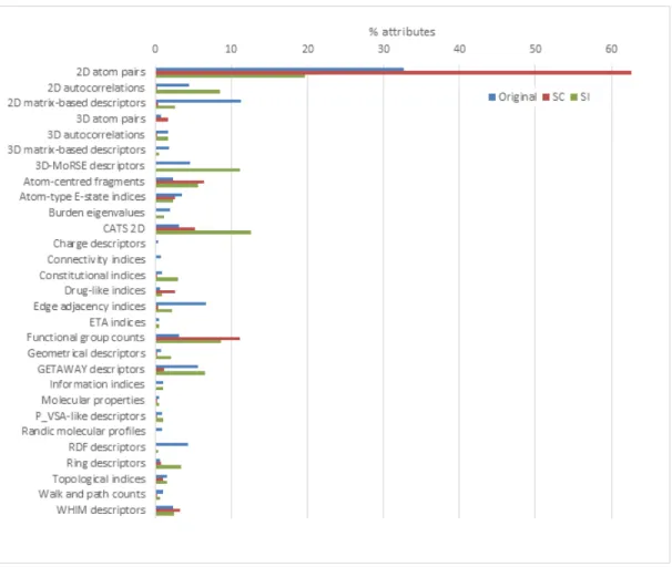
All attributes are uniquely categorized within the Dragon soft-ware into 29 attribute families. Fig. 3 and 4 show how those families are distributed within the different sets, with weights in percent-ages for S2–4 being defined as the average value between S2, S3 and S4. Table 3 summarizes the results of Chordalysis-based selection, and also highlights the overlap between SC and S2–4.
2D atom pairs are by far the most prevalent family in all cases, accounting to 33, 63 and 20% of the total attributes population in the original, SC and S2–4 sets respectively. It is very clear that Chordalysis privileged this family, now twice as present in SC compared to the original set, while on the contrary, it is significantly less important in S2–4.
The atom-centred fragments, CATS 2D and functional group counts families were not prevalent in the original set (2, 3, and 3% respectively), and become over-selected in all reduced sets, with
Figure 3: The distribution of families in 4885 original attributes, 595 attributes of SC, and around 500 attributes of S2–4.
Table 2: Intersections of the sets of attributes from three fil-ters and from Chordalysis.
Set S2 S3 S4 SC (595 attr.) 153 154 146
S2 (576 attr.) 569 497 S3 (588 attr.) 496 S4 (524 attr.)
CATS 2D being more prevalent in S2–4 compared to SC. These 3 sets account for 23% of SC, so with the addition of 2D atom pairs only 15% is remaining.
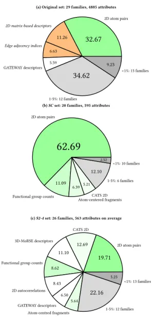
The relative diversity of the different sets can be compared by focusing on the number of families accounting for more than 5% of the total number of attributes and on their total weight (see Figure 8). Only the 4 aforementioned families obey these criteria in SC, totaling 85% of the set. There are 7 families with more in S2–4 (73%); 4 in the original set (56%). Therefore, three attribute families are seen significantly more prevalent in S2–4 compared to the original set (26% / 15%), but are almost completely filtered out by Chordalysis: 2D autocorrelations, 3D-MoRSE and GETAWAY descriptors.
Table 3: Population of most relevant attribute families. Last column is the number of attributes present in all sets (SC, S2, S3 and S4). Percentages correspond to the number of re-tained attributes from the original set.
Attribute family Original set SC Overlap 2D atom pairs 1596 373 (23%) 80 2D matrix-based 550 2 1 Edge adjacency ind. 324 2 1
GATEWAY 273 7 1 Functional group cnt. 154 66 (43%) 24 CATS 2D 150 31 (21%) 19 Atom-centered frag. 115 38 (33%) 10 Drug-like indices 27 15 (56%) 1 TOTAL 4885 595 (12%) 144 (3%)
Apart from these families, there is a consensus between S2–4 and SC regarding the removal of some attribute families from the original set, with SC appearing more stringent than S2–4. Indeed, the 2D matrix-based descriptors, edge adjacency indices and RDF descriptors account together for 22, <1 and 5% in the original, SC and S2–4 sets respectively. This suggests that those descriptors
2D atom pairs
32.67
2D matrix-based descriptors11.26
Edge adjecency indices 6.63 GATEWAY descriptors 5.59 1-5%: 12 families
34.62
<1%: 13 families 9.23(a) Original set: 29 families, 4885 attributes
2D atom pairs
62.69
Functional group counts
11.09 Atom-centered fragments 6.39 CATS 2D 5.21 1-5%: 6 families 12.10 <1%: 10 families 2.52
(b) SC set: 20 families, 595 attributes
2D atom pairs 19.71 CATS 2D 12.69 3D-MoRSE descriptors 11.10
Functional group counts
8.62 2D autocorrelations 8.43 GATEWAY descriptors 6.50 Atom-centred fragments 5.64 1-5%: 12 families 22.16 <1%: 13 families 5.25
(c) S2-4 set: 26 families, 563 attributes on average
Figure 4: Distribution of major attribute families in (a) the original set, (b) set SC, and (c) average of S2, S3, and S4. All values in percentages. Only sets weighting >5% are repre-sented. Categories in green are the 4 most-represented in SC. Those in orange with description in italic are mostly filtered out of both SC and S2–4. Grey ones summarize remaining families (1–5% and <1%).
are not of much value for modeling the probability that a given chemical compound would possess antibacterial properties.
Eventually, it should be noticed that while SC size compared to the original set is 12%, only a single attribute family has been filtered less than 50%: drug-like indices. This is specific to SC (5 attributes are retained by S2, S3 and S4). There were only 27 residues of this kind in the original set, which is not significant enough to determine that there could be a correlation between drug-likeness
Table 4: Means and standard deviations of classifiers’ met-rics on the test set. All data in percentages.
Metric SVM (C= 0.01) Random Forest Naive Bayes Accuracy 97.0 ± 2.5 96.6 ± 1.5 55.7 ± 1.4 Recall 98.9 ± 2.0 95.6 ± 1.5 21.2 ± 0.6 Precision 95.9 ± 3.5 98.3 ± 2.2 93.7 ± 9.1 AUC 99.3 ± 1.1 99.5 ± 0.4 65.3 ± 4.5 f 1scor e 97.3 ± 2.2 96.9 ± 1.3 34.5 ± 1.0
Table 5: Precision and recall of random forest classifier on the test set. All values in percentages.
α 4532 attributes SC Precision Recall Precision Recall 10 10.0 71.2 11.6 65.4 20 10.7 68.4 11.8 64.5 30 11.8 65.4 12.2 63.5 40 11.8 65.4 12.2 63.5 50 12.3 64.3 12.3 63.0 60 13.3 61.5 12.6 62.4 70 14.1 60.1 12.8 61.8 80 14.1 60.1 12.8 61.8 90 15.1 59.1 13.0 61.2 100 16.6 56.3 13.3 60.1
and antibacterial potency that would be most efficiently selected by Chordalysis.
Table 2 lists the number of overlapping selected attributes from S2, S3 and S4 with SC. Table 3 summarizes SC-related data for most-relevant attribute families identified above, and highlights the number of consensus attributes i.e. attributes found in all sets. 3.4.2 Training/testing strategy. Using attributes in SC, we trained SVM, random forest, and naive Bayes on data from market antibac-terials, MDDR antibacantibac-terials, Life Chemicals non-antibacantibac-terials, and MDDR non-antibacterials. After the training process, the three clas-sifiers are tested on Life Chemicals list of predicted antibacterials. The results are summarized in Table 4. By tuning the parameter C for SVM, we get the best result for C= 0.01.
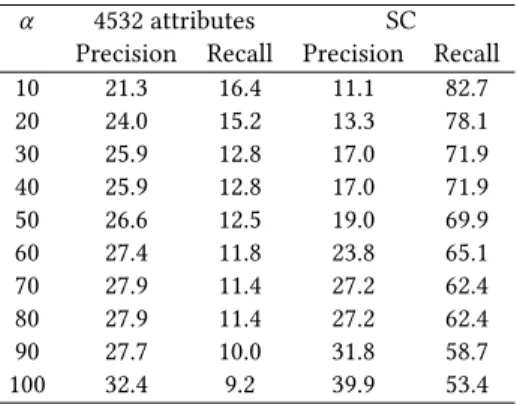
Based on the values of all metrics used to evaluate classifier performance, it appears that SVM and RF perform significantly better than naive Bayes. The two best performing model –SVM and random forest– were then trained on the market antibacterials and Life Chemical antibacterials to test the MDDR data. We regarded a molecule as an antibacterial if it is classified as such in at least α percent of runs. The precision and recall of the two models are shown in Table 5–6. SVM has better recall on the majority of alphas, and it has higher precision for α ≥ 20.
4
CONCLUDING REMARKS
We evaluated several popular classification methods, including SVM, LR, and RF, for classifying molecules as antibacterial or non-antibacterial. Such machine learning approaches were already suc-cessfully used for drug/non-drug classification [8, 17, 21, 29], but
Table 6: Precision and recall of SVM classifier on the test set. All values in percentages.
α 4532 attributes SC Precision Recall Precision Recall 10 21.3 16.4 11.1 82.7 20 24.0 15.2 13.3 78.1 30 25.9 12.8 17.0 71.9 40 25.9 12.8 17.0 71.9 50 26.6 12.5 19.0 69.9 60 27.4 11.8 23.8 65.1 70 27.9 11.4 27.2 62.4 80 27.9 11.4 27.2 62.4 90 27.7 10.0 31.8 58.7 100 32.4 9.2 39.9 53.4
none were applied to antibacterials. Along with our initial 4532 at-tribute data set (F0), we tested 4 reduced sets (F1-F4), filtered on the basis of data variance and correlation. Using those was not found to improve performance. When looking at precision as our main metric, our results show that the SVM classifier with a tuned C parameter ranks first but has much lower accuracy and f 1scor e. For
a dataset of potential antibacterial molecules, SVM could be used to find a reliable list of antibacterial molecules. Another method like RF with lower precision but better accuracy and f 1scor emay
be used if a greater number of classified antibacterials is desired. Previous investigations of the merit and drawbacks of several learning methods [20, 23, 33, 37, 45] are in good general agreement with our own observations. In future work, we should favor the use of SVM and RF over the other classifiers evaluated here in order to perform virtual screening of chemical databases for finding most probable antibacterials.
One important finding of this work is that for such a task, the choice of the classifier appears to have much more impact than the selection of molecular descriptors. We have chosen to evaluate all available descriptors from the Dragon software, without any consideration of the relative relevance of each of those. This “blind” approach has the advantage of being totally unbiased, but puts more stress on the classifiers.
Furthermore, in Section 3, we describe the application of the Chordalysis technique for molecular attribute set reduction. We show that it leads to improved performance when a machine learn-ing technique is used next to discriminate between antibacterials and compounds with no antibacterial activity. It is suggested that a two-step strategy, with a Chordalysis-refined attribute set being fed to a SVM classifier could be highly efficient for antibacterials identification. An alternate techniques for selecting an optimal at-tribute set [42], such as recursive feature elimination [18, 47], RF variable importance [9], SVM variable selection [10], tabu search [41, 48], and evolutionary algorithms [15] should be further studied. In the process, precise clues on implementing new attributes that could be more efficient for our purpose (antibacterials selection) than the broad generic reference set of molecular attributes that is available in the Dragon software could be obtained. When we reach a state where no clear methodological improvement could be
reached, we will apply the optimized methodology to mine chemi-cal space for possible new antibacterials. A limited number of hits from this virtual screening process will be tested experimentally. Only interesting results backed up by the resulting experimental data will validate the ongoing chemoinformatics approach.
REFERENCES
[1] 2004. Life Chemicals. http://www.lifechemicals.com/.
[2] 2007. Molecular Descriptors. http://www.moleculardescriptors.eu/.
[3] 2016. BIOVIA Databases | Bioactivity Databases: MDDR. http://accelrys.com/products/collaborative-science/databases/bioactivity-databases/mddr.html.
[4] Jürgen Bajorath. 2013. Chemoinformatics for Drug Discovery. John Wiley & Sons. [5] Theresa Braine. 2011. Race against time to develop new antibiotics. World Health
Organization.
[6] Leo Breiman. 2001. Random forests. Machine Learning 45, 1 (2001), 5–32. [7] L Buitinck, G Louppe, M Blondel, F Pedregosa, A Mueller, O Grisel, V Niculae,
P Prettenhofer, A Gramfort, J Grobler, et al. 2013. ECML PKDD Workshop: Languages for Data Mining and Machine Learning. API Design for Machine Learning Software: Experiences from the Scikit-Learn Project (2013), 108–122. [8] Evgeny Byvatov, Uli Fechner, Jens Sadowski, and Gisbert Schneider. 2003.
Com-parison of support vector machine and artificial neural network systems for drug/nondrug classification. Journal of Chemical Information and Computer Sciences 43, 6 (2003), 1882–1889.
[9] Gaspar Cano, Jose Garcia-Rodriguez, Alberto Garcia-Garcia, Horacio Perez-Sanchez, Jón Atli Benediktsson, Anil Thapa, and Alastair Barr. 2017. Automatic selection of molecular descriptors using random forest: Application to drug discovery. Expert Systems with Applications 72 (2017), 151–159.
[10] Chih-Chung Chang and Chih-Jen Lin. 2011. LIBSVM: A library for support vector machines. ACM Transactions on Intelligent Systems and Technology (TIST) 2, 3 (2011), 1–27.
[11] Corinna Cortes and Vladimir Vapnik. 1995. Support-vector networks. Machine Learning 20, 3 (1995), 273–297.
[12] Ezekiel J Emanuel. 2015. How to Develop New Antibiotics. New York Times, February 24th.
[13] Usama Fayyad, Gregory Piatetsky-Shapiro, and Padhraic Smyth. 1996. From data mining to knowledge discovery in databases. AI Magazine 17, 3 (1996), 37–37. [14] Prabhavathi Fernandes. 2015. The global challenge of new classes of antibacterial
agents: an industry perspective. Current Opinion in Pharmacology 24 (2015), 7–11.
[15] Alex A. Freitas. 2003. Advances in Evolutionary Computing.
[16] Jerome H Friedman. 2001. Greedy function approximation: a gradient boosting machine. Annals of Statistics (2001), 1189–1232.
[17] Alireza Givehchi and Gisbert Schneider. 2004. Impact of descriptor vector scal-ing on the classification of drugs and nondrugs with artificial neural networks. Journal of Molecular Modeling 10, 3 (2004), 204–211.
[18] Isabelle Guyon, Jason Weston, Stephen Barnhill, and Vladimir Vapnik. 2002. Gene selection for cancer classification using support vector machines. Machine Learning 46, 1-3 (2002), 389–422.
[19] Trevor J Howe, Guy Mahieu, Patrick Marichal, Tom Tabruyn, and Pieter Vugts. 2007. Data reduction and representation in drug discovery. Drug Discovery Today 12, 1-2 (2007), 45–53.
[20] Andreas Janecek. 2009. Efficient feature reduction and classification methods. Ph.D. Dissertation. University of Vienna.
[21] Selcuk Korkmaz, Gokmen Zararsiz, and Dincer Goksuluk. 2014. Drug/nondrug classification using support vector machines with various feature selection strate-gies. Computer Methods and Programs in Biomedicine 117, 2 (2014), 51–60. [22] P-J L’Heureux, Julie Carreau, Yoshua Bengio, Olivier Delalleau, and Shi Yi Yue.
2004. Locally Linear Embedding for dimensionality reduction in QSAR. Journal of Computer-aided Molecular Design 18, 7-9 (2004), 475–482.
[23] Wenwen Lian, Jiansong Fang, Chao Li, Xiaocong Pang, Ai-Lin Liu, and Guan-Hua Du. 2016. Discovery of Influenza A virus neuraminidase inhibitors using support vector machine and Naïve Bayesian models. Molecular Diversity 20, 2 (2016), 439–451.
[24] Ying Liu. 2004. A comparative study on feature selection methods for drug discovery. Journal of Chemical Information and Computer Sciences 44, 5 (2004), 1823–1828.
[25] Maryn McKenna. 2014. The coming cost of superbugs: 10 million deaths per year. https://www.wired.com/2014/12/oneill-rpt-amr/.
[26] Tom M Mitchell. 1997. Machine Learning. McGraw-Hill New York.
[27] Carl Nathan and Otto Cars. 2014. Antibiotic resistance—problems, progress, and prospects. New England Journal of Medicine 371, 19 (2014), 1761–1763. [28] Fabian Pedregosa, Gaël Varoquaux, Alexandre Gramfort, Vincent Michel,
Bertrand Thirion, Olivier Grisel, Mathieu Blondel, Peter Prettenhofer, Ron Weiss, Vincent Dubourg, et al. 2011. Scikit-learn: Machine learning in Python. The
Journal of Machine Learning Research 12 (2011), 2825–2830.
[29] Ayca C Pehlivanli, Okan K Ersoy, and Turgay Ibrikci. 2008. Drug/nondrug classification with consensual Self-Organising Map and Self-Organising Global Ranking algorithms. International Journal of Computational Biology and Drug Design 1, 4 (2008), 434–445.
[30] François Petitjean, Lloyd Allison, and Geoffrey I Webb. 2014. A statistically efficient and scalable method for log-linear analysis of high-dimensional data. In 2014 IEEE International Conference on Data Mining. IEEE, 480–489.
[31] François Petitjean and Geoffrey I Webb. 2015. Scaling log-linear analysis to datasets with thousands of variables. In Proceedings of the 2015 SIAM International Conference on Data Mining. SIAM, 469–477.
[32] François Petitjean, Geoffrey I Webb, and Ann E Nicholson. 2013. Scaling log-linear analysis to high-dimensional data. In 2013 IEEE International Conference on Data Mining. IEEE, 597–606.
[33] Vijay Rathod, Vilas Belekar, Prabha Garg, and Abhay T Sangamwar. 2016. Classi-fication of Human Pregnane X Receptor (hPXR) Activators and Non-Activators by Machine Learning Techniques: A Multifaceted Approach. Combinatorial Chemistry & High Throughput Screening 19, 4 (2016), 307–318.
[34] Matthew J Renwick, David M Brogan, and Elias Mossialos. 2014. A Critical Assessment of Incentive Strategies for Development of Novel Antibiotics. LSE Health, London School of Economics and Political Science.
[35] Michael Reutlinger and Gisbert Schneider. 2012. Nonlinear dimensionality reduc-tion and mapping of compound libraries for drug discovery. Journal of Molecular Graphics and Modelling 34 (2012), 108–117.
[36] Jens Sadowski, Johann Gasteiger, and Gerhard Klebe. 1994. Comparison of automatic three-dimensional model builders using 639 X-ray structures. Journal of Chemical Information and Computer Sciences 34, 4 (1994), 1000–1008. [37] Mohammad Shahid, Muhammad Shahzad Cheema, Alexander Klenner, Erfan
Younesi, and Martin Hofmann-Apitius. 2013. SVM based descriptor selection and classification of neurodegenerative disease drugs for pharmacological modeling. Molecular Informatics 32, 3 (2013), 241–249.
[38] S Sirois, CM Tsoukas, Kuo-Chen Chou, Dongqing Wei, C Boucher, and GE Hatza-kis. 2005. Selection of molecular descriptors with artificial intelligence for the understanding of HIV-1 protease peptidomimetic inhibitors-activity. Medicinal Chemistry 1, 2 (2005), 173–184.
[39] Brad Spellberg. 2014. The future of antibiotics. Critical care 18, 3 (2014), 228. [40] Barbara G Tabachnick, Linda S Fidell, and Jodie B Ullman. 2007. Using Multivariate
Statistics. Vol. 5. Pearson Boston, MA.
[41] Muhammad Atif Tahir, Ahmed Bouridane, and Fatih Kurugollu. 2007. Simultane-ous feature selection and feature weighting using Hybrid Tabu Search/K-nearest neighbor classifier. Pattern Recognition Letters 28, 4 (2007), 438–446.
[42] Jiliang Tang, Salem Alelyani, and Huan Liu. 2014. Feature selection for clas-sification: A review. Data Clasclas-sification: Algorithms and Applications (2014), 37.
[43] Roberto Todeschini and Viviana Consonni. 2009. Molecular Descriptors for Chemoinformatics. Vol. 41. John Wiley & Sons.
[44] L Vidal. 2016. Dictionnaire Vidal 2016 (French PDR - Physician’s Desk Reference). French and European Publications Inc., New York City.
[45] Renu Vyas, Sanket Bapat, Esha Jain, Sanjeev S Tambe, Muthukumarasamy Karthikeyan, and Bhaskar D Kulkarni. 2015. A study of applications of machine learning based classification methods for virtual screening of lead molecules. Combinatorial Chemistry & High Throughput Screening 18, 7 (2015), 658–672. [46] Geoffrey I Webb. 2008. Layered critical values: a powerful direct-adjustment
approach to discovering significant patterns. Machine Learning 71, 2-3 (2008), 307–323.
[47] Y. Xue, Z. R. Li, C. W. Yap, L. Z. Sun, X. Chen, and Y. Z. Chen. 2004. Effect of molecular descriptor feature selection in support vector machine classification of pharmacokinetic and toxicological properties of chemical agents. Journal of Chemical Information and Computer Sciences 44, 5 (2004), 1630–1638. [48] Hongbin Zhang and Guangyu Sun. 2002. Feature selection using tabu search
method. Pattern Recognition 35, 3 (2002), 701–711.
Table 7: Means and standard deviations of precision metrics of all classifiers. All values are in percentages.
Attribute set F0 (full Dragon set)
SVM (C= 10−5) LR (C= 10−2) RF GBT DT NB Precision 100.0 ± 0.0 97.2 ± 2.5 97.1 ± 25 94.6 ± 3.6 89.3 ± 3.8 83.6 ± 5.2 Accuracy 67.7 ± 2.8 95.0 ± 2.2 95.2 ± 20 94.2 ± 2.4 89.2 ± 3.0 87.1 ± 4.1 f 1scor e 52.1 ± 5.9 94.8 ± 2.5 95.1 ± 21 94.2 ± 2.4 89.2 ± 3.1 87.8 ± 3.5 AUC 86.3 ± 5.1 97.9 ± 1.6 98.9 ± 07 98.5 ± 1.3 89.2 ± 3.0 87.3 ± 4.1 F1 SVM (C= 10−3) LR (C= 10−3) RF GBT DT NB Precision 95.1 ± 2.8 92.8 ± 3.6 94.6 ± 4.1 92.1 ± 3.4 79.1 ± 4.3 92.5 ± 5.0 Accuracy 88.2 ± 2.5 88.7 ± 2.5 91.9 ± 3.0 90.4 ± 3.0 78.9 ± 3.8 77.5 ± 4.2 f 1scor e 87.2 ± 3.0 88.1 ± 2.9 91.7 ± 3.1 90.2 ± 3.1 78.8 ± 4.2 72.5 ± 6.2 AUC 94.8 ± 2.0 94.5 ± 1.9 97.3 ± 1.3 96.4 ± 1.9 78.9 ± 3.8 90.0 ± 3.6 F2 SVM (C= 10−4) LR (C= 10−6) RF GBT DT NB Precision 99.6 ± 1.1 98.8 ± 1.5 97.0 ± 2.7 96.5 ± 2.5 89.2 ± 4.8 85.5 ± 4.7 Accuracy 86.9 ± 3.2 89.3 ± 3.9 95.1 ± 2.5 95.3 ± 1.9 88.7 ± 4.0 88.5 ± 3.7 f 1scor e 84.8 ± 4.2 88.0 ± 4.1 95.0 ± 2.6 95.3 ± 1.9 88.6 ± 4.2 89.0 ± 3.5 AUC 96.0 ± 1.8 95.7 ± 2.2 98.9 ± 0.9 98.8 ± 0.9 88.7 ± 4.0 89.7 ± 3.9 F3 SVM (C= 10−4) LR (C= 10−6) RF GBT DT NB Precision 99.3 ± 1.5 98.3 ± 2.2 96.5 ± 2.3 96.2 ± 2.4 88.6 ± 5.0 86.6 ± 4.8 Accuracy 87.3 ± 2.7 88.9 ± 3.1 94.8 ± 2.3 95.2 ± 1.8 88.6 ± 3.8 89.0 ± 3.3 f 1scor e 85.4 ± 3.4 87.6 ± 3.8 94.7 ± 1.8 95.1 ± 1.9 88.7 ± 3.8 89.4 ± 3.2 AUC 96.4 ± 1.5 95.6 ± 1.9 98.6 ± 0.9 98.8 ± 0.8 88.6 ± 3.9 91.0 ± 3.3 F4 SVM (C= 10−4) LR (C= 10−5) RF GBT DT NB Precision 99.6 ± 1.0 98.7 ± 1.8 97.4 ± 2.1 96.3 ± 2.3 88.4 ± 5.0 86.3 ± 5.4 Accuracy 86.2 ± 2.5 88.5 ± 3.4 95.3 ± 2.0 95.1 ± 1.8 88.0 ± 3.5 88.6 ± 4.3 f 1scor e 83.9 ± 3.3 87.0 ± 4.3 95.2 ± 2.1 95.0 ± 1.9 88.0 ± 3.4 89.1 ± 4.0 AUC 96.4 ± 1.9 95.5 ± 2.2 98.8 ± 0.8 98.9 ± 0.7 88.0 ± 3.5 90.5 ± 3.8 10
Table 8: The proportion, precision, and recall of MDDR molecules correctly classified1using SVM, LR, and RF. All values are in percentages.
SVM α P22 N12 N22 N32 N42 Precision Recall 10 16.2 98 88.9 94.4 90.4 8.7 16.2 20 15.1 98.6 96.4 98.7 98.1 29.4 15.1 30 13.5 100 100 100 100 100 13.5 40 13.5 100 100 100 100 100 13.5 50 13.2 100 100 100 100 100 13.2 60 11.4 100 100 100 100 100 11.4 70 17 100 100 100 100 100 17 80 17 100 100 100 100 100 17 90 10.2 100 100 100 100 100 10.2 100 9.5 100 100 100 100 100 9.5 Logistic Regression α P2 N1 N2 N3 N4 Precision Recall 10 70 0 0 0 0 3.4 70 20 66.6 0 0 0 0 3.2 66.6 30 63.2 0 0 0 0 3.1 63.2 40 63.2 0 0 0 0 3.1 63.2 50 61.7 0 0 0 0 3.0 61.7 60 59.1 0 0 0 0.2 3.0 59.1 70 57.4 0 0 0 93.5 6.1 57.4 80 57.4 0.2 0.1 0.1 100 6.7 57.4 90 55.1 69.1 68.6 80 100 23.3 55.1 100 51.2 91.3 88.2 94.5 100 48.7 51.2 Random Forest α P2 N1 N2 N3 N4 Precision Recall 10 71.5 77.2 70.5 76.2 67.4 18 71.5 20 68.9 79.9 67.7 73.3 67.4 10.2 68.9 30 65.6 84.3 74.4 79.6 77 11.2 65.6 40 65.6 84.3 74.4 79.6 77 11.2 65.6 50 64.4 85.4 76 87 73 11.8 64.4 60 61.7 87.6 80.6 84.3 74.9 12.5 61.7 70 60.4 88.6 80.6 84.3 74.9 12.3 60.4 80 60.4 88.6 79.1 83.1 74.9 12.3 60.4 90 58.5 90 84.2 87.6 76.6 13.2 58.5 100 54.9 91.1 82.2 85.7 76.6 12.1 54.9
1A molecule is regarded as an antibacterial if it is classified
as such in at least α % of runs.
2P2, N1, N2, N3, and N4 refer to the antibacterial, analgesic,
cardio, antagonist, and inhibitor MDDR subsets respec-tively.