HAL Id: hal-00267523
https://hal.archives-ouvertes.fr/hal-00267523
Submitted on 27 Mar 2008
HAL is a multi-disciplinary open access
archive for the deposit and dissemination of
sci-entific research documents, whether they are
pub-lished or not. The documents may come from
teaching and research institutions in France or
abroad, or from public or private research centers.
L’archive ouverte pluridisciplinaire HAL, est
destinée au dépôt et à la diffusion de documents
scientifiques de niveau recherche, publiés ou non,
émanant des établissements d’enseignement et de
recherche français ou étrangers, des laboratoires
publics ou privés.
Convex Structuring Element Decomposition for Single
Scan Binary Mathematical Morphology
Nicolas Normand
To cite this version:
Nicolas Normand. Convex Structuring Element Decomposition for Single Scan Binary
Mathemat-ical Morphology. Discrete Geometry for Computer Imagery, Nov 2003, Napoli, Italy. pp.154-163,
�10.1007/b94107�. �hal-00267523�
Convex Structuring Element Decomposition for Single Scan Binary
Mathematical Morphology
Nicolas Normand
IRCCyN/IVC UMR CNRS 6597
Abstract. This paper presents a structuring element decomposition method and a corresponding
mor-phological erosion algorithm able to compute the binary erosion of an image using a single regular pass whatever the size of the convex structuring element.
Similarly to classical dilation-based methods, the proposed decomposition is iterative and builds a growing set of structuring elements. The novelty consists in using the set union instead of the Minkowski sum as the elementary structuring element construction operator. At each step of the construction, already-built elements can be joined together in any combination of translations and set unions. There is no restrictions on the shape of the structuring element that can be built. Arbitrary shape decompo-sitions can be obtained with existing genetic algorithms with an homogeneous construction method. This paper, however, addresses the problem of convex shape decomposition with a deterministic method.
@inproceedings{normand2003dgci, Author = {Normand, Nicolas},
Booktitle = {Discrete Geometry for Computer Imagery}, Date = {2003-11-18},
Doi = {10.1007/b94107},
Editor = {Nystr{\"o}m, Ingela and Sanniti di Baja, Gabriella and Svensson, Stina}, Keywords = {Morphologie math{\’e}matique},
Month = nov, Pages = {154-163},
Publisher = {Springer Berlin / Heidelberg}, Series = {Lecture Notes in Computer Science},
Title = {Convex Structuring Element Decomposition for Single Scan Binary Mathematical Morphology},
Volume = {2886}, Year = {2003} }
Convex Structuring Element Decomposition for
Single Scan Binary Mathematical Morphology
Nicolas Normand
IRCCyN-IVC (CNRS UMR 6597) ´
Ecole polytechnique de l’universit´e de Nantes
La Chantrerie, rue Christian Pauc, BP 50609, 44306 Nantes Cedex 3 France
Abstract. This paper presents a structuring element decomposition method and a corresponding morphological erosion algorithm able to compute the binary erosion of an image using a single regular pass what-ever the size of the convex structuring element.
Similarly to classical dilation-based methods [1], the proposed decompo-sition is iterative and builds a growing set of structuring elements. The novelty consists in using the set union instead of the Minkowski sum as the elementary structuring element construction operator. At each step of the construction, already-built elements can be joined together in any combination of translations and set unions. There is no restric-tions on the shape of the structuring element that can be built. Arbitrary shape decompositions can be obtained with existing genetic algorithms [2] with an homogeneous construction method. This paper, however, ad-dresses the problem of convex shape decomposition with a deterministic method.
1
Introduction
Mathematical morphology operators are time-consuming with large structuring elements and brute force algorithms. In the past, several methods have been described to reduce the cost of these operators. Two main approaches exist, the first one uses a decomposition of a large structuring element into a set of smaller ones. The result is obtained by a series of operations with small struc-turing elements. The overall cost is then directly connected to the number of operations and depends on the size of the initial structuring element. The sec-ond one consists in binarizing a distance map, which can be computed in a fixed number of image scans. It requires the structuring element to be expressed as a distance disk but then the computational cost is constant whatever the size of the structuring element.
The method proposed here is based on a new generalized distance transform (GDT). The algorithm is quite similar to local distance propagation algorithms but in our case, distance increments are not constant over disks size, which allows for much more flexibility in the disk construction. As an example, we describe an algorithm to decompose any convex 2D polygon in a series of pseudo-distance disks for single scan distance map computation.
The overall cost of the mathematical morphology operators derived from this GDT is constant with the size of the structuring element. Moreover, they can be used in a pipeline fashion and have very low memory requirements. In section 2 existing structuring element decomposition methods will be recalled.
2
Distances and Structuring Elements
2.1 Mathematical Morphology Operators
Let A and B be two sets of points in the discrete grid E with origin O, the neutral element for the symetry in E (p symetric element is denoted as ˇp). The erosion of A by the structuring element B is defined as:
A! ˇB ={p| (B)p⊆ A} (1)
where (B)p is B translated by p: (B)p= {x + p|x ∈ B}.
The erosion dual operator, the dilation can be defined as:
A⊕ ˇB = (Ac! ˇB)c = {p| (B)p∩ A &= ∅}. (2)
The notation ⊕ denotes the Minkowski sum of two sets i.e. the set of sums of two elements, one taken from the first set the other from the second one.
These basic operators lead to a great variety of image transformations [3]. However, the algorithm directly derived from the fundamental definition given in (eq. 1) is not efficient for a large structuring element B, as it requires the exploration of all translated points of B for each point of the image.
2.2 Distance Map
The distance transform associates to any point x the smallest distance to a point outside the set X:
dX(x) = min
y!∈X(d(x, y)) (3)
The distance map is linked to the mathematical morphology erosion by the fact that the set of points whose distance map values are at least r is the eroded set of X by D(r):
A! ˇD(r) ={p|dX(p) ≥ r} (4)
with D(r) = {p|d(O, p) < r}. Eroding a shape from a distance map consists in thresholding distance values, so the erosion cost depends only on the cost of the distance transform. Since algorithms exist to compute a distance map in a fixed number of scans [4–6], they can be used to erode with a constant cost whatever the size of the structuring element.
For usual distances, each disk is constructed by the dilation of the previous disk with a basic structuring element as illustrated in fig. 1.a. In a sequential distance map computation, the symetric neighborhood is divided in two halves which are passed over the image once, in reverse order scans [4].
By moving the morphological center of the disks to the last scanned pixel, some one-pass algorithms can be obtained [7]. We can not refer to these disks as distance disks since the symetry property of distances is not verified anymore. Hence the transform is called a generalized distance transform (GDT). However, there is a strong constraint on the shape of the disks since the basic structuring element is unique for the whole set of disks, so this method will only apply to very specific structuring elements.
By mixing different structuring elements, distances like the octagonal dis-tance add some variability: each disk can be built from the previous by a differ-ent structuring elemdiffer-ent (fig. 1.b). Any shape that is decomposed in a series of dilations can be constructed with this method. However, distance transfom al-gorithms are only known for some specific cases (for instance when two building structuring elements are used periodically [7, 8]).
On the other side, another way of mixing different neighborhoods is used in chamfer distances (fig. 1.c): each disk is built from different-size disks according to local distances described in a neighborood mask.
2.3 Structuring Element Decomposition
The structuring element decomposition methods rely on the fact that a series of erosions with a set of structuring elements is equivalent to a single erosion with the Minkowski sum of the structuring elements:
(A ! ˇB)! ˇC = A! ( ˇB⊕ ˇC). (5)
Decomposition methods generally use a series of basic structuring elements com-putable by specific hardware machines in one clock cycle. The shape of the build-ing structurbuild-ing elements depends on the hardware platform and convex polygon decomposition algorithms were presented for instance for linear shaped build-ing structurbuild-ing elements [9] and for 4 and 8-neighborhood parallel machines [1]. These decompositions lead to optimal morphological operator implementations for parallel or pipeline architectures, but conversely to distance-based methods, the computational complexity depends on the size of the structuring element.
Since some convex polygonal structuring elements can not be decomposed by Minkowski sums, an extra final set union can be needed as displayed in fig. 1.d [10]. In this case, the initial decomposition can be obtained from a single scan GDT. However, the complexity of the last step depends on the shape of the structuring element. Other methods use a fixed number of scans, but are still restricted to simple shapes such as lines [11] or rectangles [12] and also need combination for other kinds of elements [13]. In order to deal with arbitrary shapes, combinatorial and genetic algorithms have been proposed [2].
3
Convex Polygon Decomposition for Single Scan Erosion
The proposed method is the combination of a construction scheme used to recur-sively build structuring elements (section 3.1), a generalized distance transform
1,2
v0
v4
Fig. 1. Some disk and structuring element construction examples. a: d4 disks (first
row). b: octagonal distance disks (second row). c: chamfer distance d2,3 disks (third
row). d: line elements obtained by a GDT are gathered in the last step (last row)
(section 3.2) and a decomposition algorithm (section 3.3) which determines how structuring elements have to be assembled to obtain a given convex polygon.
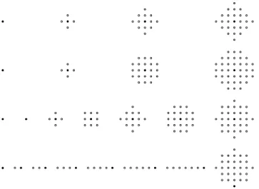
A sample polygon P is shown in fig. 2. It is convex since it is equal to the intersection of all the half-planes supported by its sides. The aim of the method is to obtain structuring element B, the discrete counterpart of P. B is the set of discrete points of the square grid included in the closed polygon P. The construction is directed by a series of increasing polygons {P(i)}i∈[2..N] used
as templates for the structuring elements assembling. Each structuring element
B(i) is the discrete counterpart of its corresponding polygonP(i), defined in the
continuous plane. ! ! ! ! ! ! ! ! ! ! ! ! ! ! ! ! ! ! ! ! ! ! ! ! ! ! ! ! ! ! ! ! ! ! ! ! ! ! ! ! ! ! ! ! ! ! ! ! ! ! ! ! ! ! ! ! ! ! ! ! ! ! ! ! ! ! ! ! ! ! ! ! ! ! ! ! ! ! ! ! ! ! ! ! ! ! ! ! ! ! " B(1) # " B(2) # # "# B(3) # # # "# # # # B(4) " !" p1 p2 ! ! ! ! ! ! ! ! ! ! ! ! ! ! ! ! ! ! ! ! ! ! ! ! ! ! ! ! ! ! ! ! ! ! ! ! ! ! ! ! ! ! ! ! ! ! ! ! ! ! ! ! ! ! ! ! ! ! ! ! ! ! ! ! ! ! ! ! ! ! ! ! ! ! ! ! ! ! ! ! ! ! ! ! ! ! ! ! ! ! " P(1) " # P(2) " # # P(3) " # # $ P(4) " !" p1 p2
Table 1. Structuring element construction table (see text concerning column 1).
i 1 2 3 4
I1(i) 0 1 2 3
I2(i) 0 0 1 3
3.1 Structuring Element Construction
Like the methods recalled in the previous section, the proposed structuring el-ement construction scheme recursively builds a family of increasing elel-ements. However, each structuring element can be built from different smaller elements (conversely to dilation-based construction) and size increments are not fixed for each neighborhood (conversely to chamfer disks). This method operation can be compared to local distance increment with varying weights.
Each structuring element B(i) is the union of smaller structuring elements translated according to a set of neighbors {pk}. For instance, in fig. 2,
B(2) = B(1)∪ (B(1))p1
B(3) = B(2)∪ (B(2))p1∪ (B(1))p2 B(4) = B(3)∪ (B(3))p1∪ (B(3))p2
where B(1) is the simplest element, only containing the origin {O}.
A general expression is given by introducing Ik(i), the index of the element
used in neighborhood pkfor B(i), B(0) the empty set and neighbor p0the origin:
∀i = 2 . . . N B(i) =!k∈[0,K](B(Ik(i)))pk (6)
The values of Ik(i) are summarized in a construction table. Such a table is shown
in table 1 for fig. 2 structuring elements. Despite B(1) is not built stricto sensu, an extra column 1 is however added for later computing purposes.
Disk increase. By adding p0 = O with I0(i) = i − 1, we have (B(Ik(i)))p0 =
B(i− 1), so B(i − 1) is always a subset of B(i). Without loss of generality, we
can assume that each Ik table contains increasing values (Ik(i) ≥ Ik(i − 1)).
Comparison with Other Methods. This construction scheme generalizes the disk
or structuring element construction methods previously recalled. Chamfer dis-tances use constant local distance increments which correspond to a fixed differ-ence between a constructed disk size i and the included disk size Ik(i). Chamfer
distance da,b is obtained with Ik(i) = i − a or Ik(i) = i − b depending on pk.
Dilation series are obtained by taking Ik(i) = i − 1 for each pk belonging to the
structuring element used to build B(i).
Each pkcan be any point in the discrete plane. The neighbor set is determined
3.2 Single Pass Generalized Distance Transform and Erosion
The value of the distance map at point x is the index of the largest structuring element centered in x contained in X. It is built from elements located on x neighbors: {x + pk}. The current element size is the greatest one that contains
all the neighbor elements:
dX(x) = max{i|∀k, Ik(i) ≤ dX(x + pk)}
= min
k {max{i|Ik(i) ≤ dX(x + pk)}}
In order to speed up the distance transform computation, we introduce Mk(j):
Mk(j) = max(i|Ik(i) ≤ j). (7)
The distance transform is then:
dX(x) =
"min
k(Mk(dX(x + pk))) if x ∈ X
0 otherwise (8)
Mk(j) represents the index of the largest element B(i) that can be built with
B(j) in the neighborhood k. Mk(j) is at least equal to 1 due to column 1 filled
with 0 in table 1. Mk can be computed once from the construction table Ik.
table 2 shows the Mk values corresponding to the example construction values
displayed in table 1
The overall complexity is linear with the number of image pixels like all GDT. Furthermore, if all the neighborhoods are chosen to be causal (all pk precede O
in the scan order) then only one image scan is needed. While it is also true for some GDT for few restricted shape classes, this GDT works with any convex polygonal shape as it will be shown in next section.
The erosion of X by B = B(N) is finally:
p∈ X ! ˇB⇔ dX(p) = N
The causality hypothesis implies that the last vertex in scan order must be equal to the origin O. The single-scan algorithm structure permits to use it in a pipeline chain, with one stage for each morphological operation (for instance, a morphological opening requires two pipeline stages). A first implementation has been realized on a Xilinx Spartan IIE FPGA educational card fed with a PAL video signal. The FPGA handles the input synchronization signal and regenerates it on the output. Due to the low cost of the algorithm, at least 8 morphological pipeline stages with different structuring elements can be handled at video rates without extra resources (only in-chip memory is used). The input-output delay is only a fraction of a pixel for each stage and an extra delay can be introduced in the output synchronization signal to compensate the translation of the structuring element center.
Table 2. Generalized distance transform table Mk. M1(1) = 2 because disk 2 can be
built with disk 1 in neighborhood 1 but disk 3 can not
j 0 1 2 3 4
M1(j) 1 2 3 4 4
M2(j) 2 3 3 4 4
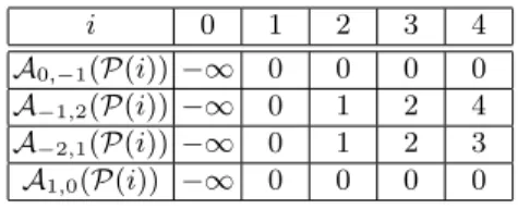
Table 3. Half-plane location table
i 0 1 2 3 4
A0,−1(P(i)) −∞ 0 0 0 0
A−1,2(P(i)) −∞ 0 1 2 4
A−2,1(P(i)) −∞ 0 1 2 3
A1,0(P(i)) −∞ 0 0 0 0
3.3 Convex Structuring Element Decomposition
The proposed structuring element construction evokes the anisotropic growth of a single crystal in which epitaxial layers of atoms are successively deposited on a crystal seed. The shape of the crystal is influenced by the physical properties of atoms which constrain the orientations and by the speed of the deposit which may differ from an orientation to another. The orientation of its sides remain constant during the growth. The shape of the structuring element is controlled by artificial constraints which maintains the direction of its sides. However, as the discrete plane produces orientation artifacts especially for small structuring element sizes, the growth is proceeded on a family of continuous polygons which are then used as templates for the structuring elements.
The decomposition method is able to process any convex polygon i.e. any closed shape that can be obtained from the intersection of half-planes. For in-stance, P(4) shown in fig. 2 is bounded by the following half-planes:
(x, y) ∈ P(4) ⇔ −y ≤ 0 −x + 2y ≤ 4 −2x + y ≤ 3 x≤ 0 ⇔ A0,−1(P(4)) ≤ 0 A−1,2(P(4)) ≤ 4 A−2,1(P(4)) ≤ 3 A1,0(P(4)) ≤ 0 (9) with: Ap,q(X) = max (x,y)∈X(px + qy)
The decomposition algorithm consists in moving the planes from their initial seed position (tangent at the origin with Apl,ql = 0) to their final position. A series of
positions is computed for all half-planes as displayed in table 3 for fig. 2 polygons. Half-planes locations are set in such a way that the sides of intermediate polygons
P(i) have a constant orientation and an increasing length:
∀i > 0, ∀j ≥ i, ||vl+1,i− vl,i|| ≥ ||vl+1,j− vl,j|| (11)
Structuring elements from polygons The index of the structuring element used in neighborhood pk is determined as the largest polygon translated by pk
that is included in P(i):
Ik(i) = max(i : (P(Ik(i)))pk⊆ P(i)
= max(i : ∀l, Apl,qlP(Ik(i)) + Apk≤ Apl,qlP(i))
This expression of Ik(i) ensures that every structuring element B(i) is a subset
of the corresponding polygon P(i): ∀i, B(i) ⊆ P(i).
Polygon set As a result of the polygon side properties (constant orientation and increasing length, eq. 10, 11), the series of polygons can be iteratively constructed by Minkowski sums in the continous plane [14]. A direct consequence on the construction is that:
vl,i= vl,j+ pk⇒ Ik(i) ≥ j
⇒ (vl,j ∈ B(j) ⇒ vl,i∈ B(i))
Therefore, if the set of intermediate vertex vl positions {vl,i}i∈[i..N] contains a
path from O to vlusing neighbor moves (plus extra non discrete positions), then
vl is necessarily contained in P. Algorithm 1 takes this point into consideration.
Half-plane positions are guided by the movement of vertices. Each vertex is initially located at the origin and follows a path to its final position using the two neighbors of its influence cone. The algorithm ensures that each position in the path is correctly reached by the half-plane, i.e. that half-plane boundaries meet exactly at the vertex intermediate positions.
Neighbor selection This phase is actually the first in the decomposition pro-cess, it must ensure that the obtained structuring elements are convex and that paths to vertices can be obtained with polygons of increasing side length (eq. 11). Each pair of successive neighbors defines an influence cone that have some similarities with chamfer disks geometry [15]. In an influence cone, each pixel is reached by a series of moves along the two neighbors. The main difference with chamfer distances is that the vertices of the structuring element do not nec-essarily belong to boundaries between cones. Therefore the number of needed neighbors is generally less than the number of vertices in P. There are two constraints on the pair of neighbors (pk, pk+1):
i all pixels from the influence cone must be reachable from the neighbors.
A necessary and sufficient condition is that pk and pk+1form a regular cone
(det[pk, pk+1] = 0) [15].
ii all pathes to a point must be included in the structuring element.
If p ∈ B(i) is in the cone (pk, pk+1) and p = apk+ bpk+1 then all the points
Algorithm 1 Half-planes shift computation
i← 0
while∃l : vi,l%= vi do
{Update reached vertices intermediate position}
for l← 1 to L do {Test of vertex vl,i}
if ∀m, Apm,qm({vl,i}) ≤ AHm then
{All half-planes contain vl,i, move it to the next intermediate location}
choose neighbor k vl,i+1← vl,i+ pk else vl,i+1← vl,i end if end for {Half-plane shift} for l← 2 to L − 1 do
{Reach the closest vertex vlor vl+1}
AHl← min(Apl,ql{vl, vl+1})
end for
i← i + 1
end while
Algorithm 2 Determination of neighbors
{Selection of the two initial neighbors} p1= (v2x/ gcd(v2x, v2y), v2y/ gcd(v2x, v2y)) p2= (vLx/ gcd(vLx, vLy), vLy/ gcd(vLx, vLy))
{Neighbor insertion for condition i}
while k < K do
if det(pk, pk+1)%= 1 then
{(pk,pk+1) is not a regular cone}
find a et b with extended Euclide’s algorithm such that bpk x− apk y= 1
n≥p bpk+1x−apk+1y
k xpk+1y−pk ypk+1x > n− 1
insert (a + npk x, b + npk y) after k (indices above k are shifted) end if
k← k + 1
end while
{Neighbor insertion for condition ii}
for n = 1 to L do
{Detection of the cone (pk,pk+1) containing vn}
while vnis not atteignable do
{division of the cone}
insert neighbor pk+pk+1 after k
if vnis in the second half-cone pk+1+pk+2(indices after insertion) then
k← k + 1
end if end while end for
4
Conclusion
We have introduced a unified structuring element construction scheme, the cor-responding generalized distance transform algorithm and a convex polygon de-composition method. Eroding an image only requires a single regular scan of the image pixels which differs from the classical chamfer distance transform by table lookups instead of constant local distant increments. The computational properties of these algorithms allow their use in a pipeline manner, optimizing time and memory consumption for series of morphological operations.
References
1. Xu, J.: Decomposition of convex polygonal morphological structuring elements into neighborhood subsets. IEEE trans. on PAMI 13 (1991) 153–162
2. Anelli, G., Broggi, A., Destri, G.: Decomposition of arbitrarily shaped binary morphological structuring elements using genetic algorithms. IEEE trans. on PAMI 20 (1998) 217–224
3. Serra, J.: Image analysis and mathematical morphology. Academic Press London (1982)
4. Rosenfeld, A., Pfaltz, J.: Distances functions on digital pictures. Pattern Recog-nition Letters 1 (1968) 33–61
5. Yokoi, S., Toriwaki, J., Fukumura, T.: On generalized distance transformation of digitized pictures. PAMI 3 (1981) 424–443
6. Borgefors, G.: Distance transformations in digital images. CVGIP 34 (1986) 344– 371
7. Wang, X., Bertrand, G.: An algorithm for a generalized distance transformation based on minkowski operations. In: ICPR. (1988) 1164–1168
8. Wang, X., Bertrand, G.: Some sequential algorithms for a generalized distance transformation based on minkowski operations. IEEE Trans. on PAMI 14 (1992) 1114–1121
9. Gong, W.: On decomposition of structure element for mathematical morphology. In: ICPR. (1988) 836–838
10. Ji, L., Piper, J., Tang, J.: Erosion and dilation of binary images by arbitrary structuring elements using interval coding. Pattern Recognition Letters (1989) 201–209
11. van Herk, M.: A fast algorithm for local minimum and maximum filters on rect-angular and octogonal kernels. Pattern Recognition Letters 13 (1992) 517–521 12. Van Droogenbroeck, M.: Algorithms for openings of binary and label images with
rectangular structuring elements. In Talbot, H., Beare, R., eds.: Mathematical morphology. CSIRO Publishing, Sydney, Australia (2002) 197–207
13. Soille, P., Breen, E., Jones, R.: Recursive implementation of erosions and dilations along discrete lines at arbitrary angles. IEEE Transactions on Pattern Analysis and Machine Intelligence 18 (1996) 562–567
14. Ohn, S.: Morphological decomposition of convex polytopes and its application in discrete image space. In: ICIP. Volume 2. (1994) 560–564
15. Thiel, E., Montanvert, A.: Chamfer masks: Discrete distance functions, geometrical properties and optimization. In: ICPR. Volume III. (1992) 244–247