Contents lists available atScienceDirect
Journal of Sound and Vibration
j o u r n a l h o m e p a g e : w w w . e l s e v i e r . c o m / l o c a t e / j s v iSecond-order moment of the first passage time of a
quasi-Hamiltonian oscillator with stochastic parametric and
forcing excitations
H. Vanvinckenroye
a,b, V. Denoël
a,*aStructural Engineering Division, Faculty of Applied Sciences, University of Liège, Liège, Belgium bFRIA (F.R.S.-F.N.R.S), National Fund for Scientific Research, Brussels, Belgium
a r t i c l e i n f o
Article history: Received 4 August 2017 Revised 1 March 2018 Accepted 2 March 2018 Available online 26 April 2018
Keywords: Stochastic stability Parametric oscillator First passage time Mathieu equation
Generalized Pontryagin equation
a b s t r a c t
This work focuses on the stochastic version of the linear Mathieu oscillator with both forced and parametric excitations of small intensity. In this quasi-Hamiltonian oscillator, the concept of energy stored in the oscillator plays a central role and is studied through the first passage time, which is the time required for the system to evolve from a given initial energy to a target energy. This time is a random variable due to the stochastic nature of the loading. The average first passage time has already been studied for this class of oscillator. However, the spread has only been studied under purely parametric excitation. Extending to combinations of both forcing and parametric excitations, this work provides a closed-form solution and a thorough analytical study of the coefficient of variation of the first passage time of the energy in this system. Simple asymptotic solutions are also derived in some particular ranges of parameters corresponding to different regimes.
© 2018 Elsevier Ltd. All rights reserved.
1. Introduction
This paper is concerned with the stochastic version of the undamped Mathieu oscillator, governed by equation
̈
x(t) + [1+u(t)]x(t) =w(t)
,
(1)subject to the forced excitation w(t)and to the parametric excitation u(t)
,
and where x(t)is the state variable as a function of time t. As an example, a vertical motion of the support of a pendulum in the gravity field generates this kind of parametric excitation while a horizontal motion generates a forcing excitation [1]. As another example, the deflection of a cable subjected to an axial oscillation of one anchorage is described by a similar Mathieu equation [2]. The rotative equilibrium of tower cranes under gusty wind can also be written in a similar format [3,4].The current work further assumes that this stochastic oscillator is submitted to small forced and parametric excitations which owes it to be classified as a quasi-Hamiltonian oscillator. For this class of oscillators, the concept of total internal energy plays a central role. It finds applications in wave energy harvesting [5–8], capsizing and rolling motions of ships under stochastic wave excitation [9,10] and several other biological applications such as protein folding [11]. Using the appropriate non-dimensionalization and discarding the nonlinear governing components, the governing equations of a large number of applications can be cast under the format of Equation(1)where u(t)and w(t)are stochastic processes.
* Corresponding author.
E-mail address:v.denoel@uliege.be(V. Denoël). https://doi.org/10.1016/j.jsv.2018.03.001 0022-460X/© 2018 Elsevier Ltd. All rights reserved.
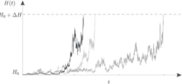
Fig. 1. Three time evolutions of the energy H of a stochastic oscillator from H0=10
−5to H=10−2with white noise excitations of intensities S
u=0.01 and Sw=0.5×10
−5.
For the considered governing equation, any large value of the generalized coordinate x is encountered with probability one in the undamped case [12]. For this reason and those that have been mentioned in Ref. [13], we investigate the time required for the system to reach a certain displacement or amplitude, given an initial condition, or to reach a given energy barrier departing from a lower initial total internal energy level. This is known as a first passage problem. As the system is stochastically excited, the first passage time is a random variable.Fig. 1presents three realizations of the energy H of the oscillator departing from a small initial energy H0and reaching a larger energy level H0+ ΔH. Each realization provides a different first passage time.
There are very few problems where the complete statistical distribution of the first passage time is available in closed form [14]. For more complex problems, even such as the problem considered here, perturbation methods or numerical techniques can be used to provide approximations of the exact solution. In particular Monte Carlo simulations, based on realizations as shown inFig. 1, are known to be versatile and accurate, although highly time consuming. Other approaches are based on the solution of the (generalized) Pontryagin equation(s) [12,15–18], sometimes with the finite difference method [19,20]; alter-native methods to determine the transient evolution of joint probability density functions include path integral approaches [21–24], smooth particle hydrodynamics or other Lagrangian methods [25], semi-analytical methods such as the Galerkin pro-jection scheme [26,27], the Poisson distribution based assumptions [28] or other applications of the perturbation method in evolutionary spectral analysis [29].
In this paper, we develop an analytical solution. Analytical methods are usually not able to determine the complete distribu-tion of the first passage time and are limited to its first few statistical moments.
In particular, the mean first passage time provides a first apprehension of the phenomenon so that many stochastic oscillators are first studied by means of their mean first passage times [30–33]. The variance of the first passage time also reflects the range of the possible observed first passage times in real conditions and is therefore interesting in a direct simulation. It also provides a valuable information as to the sample distribution of the mean first passage time, as it depend on the parent distribution of this random variable. With this respect, confidence intervals of observed mean first passage times basically depend on the spread of this random variable.
In this paper, we further restrict the considered problem to cases where u(t)and w(t)are
𝛿
-correlated processes. Under this limitation and considering the system to be quasi-Hamiltonian, closed-form solutions exist for the distribution of the first passage time in the undamped configuration (𝜉
=0) and without external forcing term (w=0) [14,34]. In this latter case, the stochastic differential equation governing the energy is a geometric differential equation. The first passage time of the energy level Hc, starting from a lower initial energy H0can be solved explicitly [14] and follows an inverse Gaussian distribution with meanS4 uln ( Hc∕H0 ) and shape-parameterS2 uln ( Hc∕H0 )2. In other or more general cases, the distribution takes very complicated expressions. In this paper, we derive a simple explicit solution for the second-order moment (variance) of the first passage time and provide corresponding solutions in the existing limiting cases, i.e. under forced excitation only or under parametric excitation only. In Section2, the considered problem is posed. It is solved, validated and discussed in Sections3 and 4.
2. Problem statement
The undamped, externally and parametrically forced oscillator is governed by the governing equation(1)where u(t)and
w(t) are
𝛿
-correlated noises of small intensities Su and Sw, such that E[u(t)u(s)] =𝛿
(t−s)Su, E[w(t)w(s)] =𝛿
(t−s)Sw andE[u(t)w(s)] =
𝛿
(t−s)Suw.Since the problem at hand is particularly interesting when the intensities of the excitations are small, the considered oscil-lator actually happens to be a quasi-Hamiltonian system for which the total internal energy (also referred to as the Hamiltonian)
H(t), defined by H=x 2 2 +
̇
x2 2,
(2)evolves on a slow time scale [15]. Indeed, the energy balance of the governing equation, obtained by time integration of the power fluxes, yields
̇
x22 +
x2
which shows that the total internal energy is slowly varying, sinceH
̇
=wẋ
−uxẋ
=ord(𝜀
)if{u,
w} =ord(𝜀
).Formally this problem is represented in the state-space𝐱 = (x
, ̇
x)by its It̂
o formulation for Markov times, i.e. for each t>
t0, by d𝐱 = 𝐟(𝐱,
t)dt+𝐛(𝐱,
t)d𝐁,
(4) where𝐱 = [ ẋ
x ],
𝐟 = [̇
x −x ] ,𝐛 = [ 0 0 −x 1 ] and where𝐁 = [ Bu Bw ]is the vector of Brownian motions characterized by the power spectrum matrix 𝐒 = [ Su Suw Suw Sw ] =
𝜀𝝂
=𝜀
[𝜈
u𝜈
uw𝜈
uw𝜈
w ],
(5)where
𝜀 ≪
1 and𝝂
is an order-one matrix.Because the considered system is stochastic, the time required to reach the total internal energy barrier H0+ ΔH, starting
from energy H0is a random variable. Its mean value has already been investigated in Ref. [13]. The objective of this study is to determine the second-order statistical moment, in order to provide some information about the spread of this statistical distribution.
3. Solution and analysis of the model
3.1. Generalized Pontryagin equations
Equation(4)is a perturbation of a conservative system which evolves along closed trajectories of constant total internal energy H. The period of revolution of a complete orbit of the unperturbed system (
𝜀
=0, so that u=w=0),T=2 x2 ∫ x1 dx
̇
x =2 √ 2H ∫ −√2H 1 √ 2H−x2dx=2𝜋,
(6)is independent of the considered energy level H. The solution of Equation(4)is therefore derived by changing the variables q and p into the energy-phase variables k and
𝜃
witḣ
x=2k cos
𝜃
; x=2k sin𝜃
(7)so that the Hamiltonian is now given by H=2k2. As the energy k evolves on slower dynamics than the phase variable
𝜃
, one can assume that the energy is constant along one period of oscillation, i.e. the system is quasi-Hamiltonian. The stochastic averaging of equation(4)over one revolution T=2𝜋
using It̂
o differential rules and Wong-Zakaï correction terms [12] provides the averaged It̂
o equation governing the time-evolution of the Hamiltonian [13,34].dH=m(H)dt+
𝜎
(H)dB(t),
(8)with m=H2Su+12Swand
𝜎
2= H2
2Su+HSwthe drift and diffusion coefficients. This stochastic differential equation in H(t)is actually the leading order solution of the general procedure proposed by Khasminiskii [35] to study the asymptotic behaviour of quasi-Hamiltonian systems. Equation(8)provides an accurate approximation for the It
̂
o equation(4)when the corresponding first passage time is much higher than the period of the oscillator given in(6).This problem is characterized by an entrance boundary class when Sw≠0 and a repulsively natural boundary when Sw=0, see Ref. [34]. The boundary class is determined through the diffusion exponent
𝛼
l, drift exponent𝛽
land character value cl. Those coefficients are given by the following limits:⎧ ⎪ ⎪ ⎨ ⎪ ⎪ ⎩
𝜎
2(H) → (|H−H l|𝛼l), 𝛼
l≥0,
H→Hl m(H) → (|H−Hl|𝛽l), 𝛽
l≥0,
H→Hl 2m(H)(H−Hl)𝛼l−𝛽l𝜎
2(H) →cl,
H→0 (9)with Dlthe left boundary for the initial state corresponding to the root of
𝜎
∶Hl=0. For Sw≠0, one finds𝛼
l=1,𝛽
l=0 andcl=1 corresponding to an entrance class and for Sw=0,
𝛼
l=2,𝛽
l=1 and cl=2 leading to a repulsively natural boundary class, as announced before.Letbe a closed domain in the phase plane defined by ={H∶0≤H≤Hc}and an initial condition H0∈. The n-th statistical moment of the first passage time Un=E[tn
1]for the trajectories of the dynamical system with drift and diffusion coefficients m and
𝜎
2to reach the boundary𝜕
is ruled by the generalized Pontryagin equation [36].1 2
𝜎
2 (H0) d 2 dH2 0 Un+m(H0) d dH0 Un= −nUn−1,
with U0=1 and n=1,
2,
3,
… (10)with H0= x
2 0+ẋ
2 0
2 and the boundary conditions [34].
Un(H0) =0
,
∀H0∈𝜕
and |Un(H0)|<
∞,
∀H0∈l.
(11)The first condition translates that the first passage time is deterministic and equal to zero for trajectories starting on the bound-ary,
𝜕
=Hc. The second condition expresses that the time (and its statistical moments) required to reach the boundary starting from H0=0 is finite. This qualitative condition can be replaced by the quantitative condition(|m(H0)U′
n(H0)|) ∼ (|U′n−1(H0)|)
,
H0→Hl (12)for entrance (Sw≠0) and repulsively natural (Sw=0) boundary classes.
3.2. Average first passage time U1
The solution U1(H0;Hc)of(10)for n=1 satisfying the boundary conditions(11) and (12), provides the average first pas-sage time for the system departing from an initial energy H0to a target energy Hc=H0+ ΔH. The general solution has been
developed and analyzed in Ref. [13]. It takes the closed form:
U1= 4 Su ln ( HcSu+2Sw H0Su+2Sw ) = 4 Su ln ( 1+ ΔH⋆ H⋆0 +1 ) (13) where the dimensionless groups
H⋆0 = H0Su
2Sw
and ΔH⋆=ΔHSu
2Sw
(14) have been defined to simplify the notations. Expression (13) highlights the existence of three different regimes [13].
Incubation regime (I). ForΔH⋆
≪
H⋆0 +1, the logarithm may be linearized and the mean first passage time can be written asU(I)1 = 4
Su
ΔH⋆
H⋆0 +1
.
(15)In this regime, the average first passage time is proportional to ΔH⋆. This is valid for U1
≪
4∕Su so that an incubation time is arbitrarily defined as Uincub=1∕2Sucorresponding to the time window during which the average first passage time scales with the energy increase ΔH⋆. Notice that a system without a parametric excitation (Su=0 and therefore H⋆0 →0 and ΔH⋆→0) is not able to experience any other regime than the incubation regime since the incubation time grows infinite.Multiplicative regime (M). When H⋆0
≫
1, the mean first passage time depends on by how much the initial energy is mul-tiplied to obtain the target energy level. In this regime, the expected first passage time does not scale withΔH⋆anymore. It is expressed asFig. 2. Second-order moment of the first passage time as a function of the target energy Hcfor different values of H0=5,10,…,40, while Su=0.1 and Sw=0.05; Monte
U(M)1 = 4 Su ln ( 1+ΔH⋆ H⋆0 ) = 4 Su lnHc H0 (16) and is independent of the forcing excitation intensity Sw. In the overlap between the multiplicative and the incubation regimes the linearized solution reads U1=S4
u
ΔH H0
.
Additive regime(A). When H⋆0
≪
1, the first passage time tends toU(A)1 = 4
Suln
(
1+ ΔH⋆) (17)
which indicates that, for large energy increases,ΔH⋆
≳
1, the average first passage time increases less than proportionally withΔH⋆. In this latter case, no matter the smallness of the initial energy H0in the system, provided it is much smaller than 2Sw∕Su, it does not influence the expected first passage time. In this regime, the expected first passage time only depends on the increase in energyΔH⋆, in other words on how much energy is added to the initial condition H0. In the overlap between the additive and the incubation regimes the linearized solution reads U1= S2
wΔ
H, which also corresponds to the limit case Su→0.
Fig. 3(a) shows the complete expression of the first passage time U1Su
4, as given by(13), as a function of H⋆andΔH⋆, and identifies the three regimes (incubation, additive and multiplicative). The curves of same expected first passage time are regularly spaced for values smaller than 0.1, which corresponds to the incubation regime where the time increases linearly with the energy increase. The left part of the diagram corresponding to the additive regime presents horizontal asymptotes as the first passage time is independent of the initial energy level. Finally, the multiplicative regime is represented in the right part where the time depends on the relative energy increaseΔH⋆∕H⋆0 and the curves present a unitary slope in logarithmic scales. Forced-and parametric-only excitations respectively correspond to the bottom left Forced-and upper right corners. As already introduced, they
Fig. 3. Representation of (a) the averageU1Su
4 with identification of the three regimes, (b) the mean square
U2S2u
32 , (c) the variance
𝜎2S2
u
32 and (d) the coefficient of variation cv.
happen to take place in the incubation and multiplicative regimes. The additive regime can only be accessed with a combination of forced and parametric excitations.
3.3. Mean square first passage time U2
This section develops and analyses the expression of the variance. The topology of the generalized Pontryagin equation(10)
is the same for all orders so that one can expect strong similarities between the average and higher moments. Indeed, the homogenous part of(10)is identical while the non-homogenous part injects the previous order solution with its characteristics. This recurrence leads to very similar features for all statistical moments. This is why the mean square and variance of the first passage time are now studied in the light of the three previously identified regimes.
Accounting for the boundary conditions(11) and (12), it might be shown that the general solution of(10)for n=2, with U1 given by(13), is U2= 32 S2 u [ ( H0Su+2Sw 2Sw ) − ( HcSu+2Sw 2Sw ) +ln ( HcSu+2Sw 2Sw ) ln ( HcSu+2Sw HcSu ) −ln ( H0Su+2Sw 2Sw ) ln ( HcSu+2Sw H0Su ) (18) +ln ( HcSu+2Sw H0Su+2Sw )]
.
The functionstands for the real part of the polylogarithmic function and is defined as
(x) =Re[Polylog(2
,
x)]= − ∫ ln(1−x)x dx ∀x
>
1.
(19)This expression for the mean square first passage time shows the relatively complex interactions between the forcing and parametric excitations. It is valid under the hypotheses that are required to separate the slow energy and the fast phase variables. These are equivalent to assuming a quasi-Hamiltonian system, or that the dimensionless intensities Suand Sware small numbers, compared to 1.
As a first validation,Fig. 2compares this analytical solution to the mean square first passage time U2obtained with Monte Carlo simulations (dots). Each curve corresponds to a different initial energy H0(H0=5
,
10,
…,
40). The numerical simulations virtually fit and validate the analytical solution, especially in the range of large mean square first passage time, i.e. where the average first passage time is large too, which is a required assumption for the stochastic averaging. For target energy levelsHcwhich are slightly larger than the initial condition H0, the stochastic averaging is no longer accurate and a boundary layer solution using Khasminskii’s approach needs to be developed, see e.g. Ref. [13].
As a second validation, we restrict to the case where there is no forcing excitation, i.e. Sw=0, so that the second-order moment is given by lim Sw→0 U2= 32 S2u ( ln ( 1+ΔH H0 ) +1 2ln ( 1+ΔH H0 )2)
.
(20)This expression corresponds to existing results in the literature [14].
3.4. Discussion on the dispersion of the first passage time
For further investigation, and similarly to the analysis of the first-order moment U1that led to the identification of the three regimes (incubation, multiplicative, additive), the mean square first passage time is rewritten in terms of the reduced initial energy and energy increase H⋆0 andΔH⋆defined in(14). Equation(18)becomes:
S2 u 32U2= [ (1+H⋆0)−(1+H0⋆+ ΔH⋆) +ln(1+H⋆0 + ΔH⋆)ln ( 1+H⋆0 + ΔH⋆ H⋆0 + ΔH⋆ ) −ln(1+H⋆0)ln ( 1+H⋆0 + ΔH⋆ H⋆0 ) (21) +ln ( 1+ ΔH⋆ 1+H⋆0 )]
.
This expression is plotted in Fig. 3(b). This formulation shows that the second-order moment of the first passage time is expressed as the product of 32
S2u
the parametric and forcing excitations Suand Swin the energetic behaviour of the stochastic oscillator as those two intensities appear as a ratio in the reduced coordinates and S2
ualso appears as a multiplicative factor, as expected from(13).
Three regimes were identified through the average first passage time. The asymptotic behaviours of the mean square first passage time in each regime can be developed:
Incubation regime. ForHΔH⋆⋆
0+1
≪
1, the mean square is given by
S2 u 32U (I) 2 = ΔH⋆ H∗ 0+1 ( 1−ln ( 1+H⋆0) H⋆0 ) (22)
Additive regime. For H⋆0
≪
1 andΔH⋆≫
1, the second-order moment becomesS2u 32U (A) 2 = −
𝜋
2 6 + ln(ΔH⋆) 2ΔH⋆ ( 4+ ΔH⋆ln(ΔH⋆))+ln(1+ ΔH⋆).
(23)As expected, the limit depends onΔH⋆only, which corresponds to the horizontal asymptotes in the left part ofFig. 3(b). This behavior was also observed in the average first passage time. The qualification “additive” therefore remains. However the additive regime is now restricted to the upper left corner, while the entire left part was covered by the asymptotic solution for the average first passage time. This means that there is no overlap between the incubation and additive regimes anymore.
Multiplicative regime. For H⋆0
≫
1, the asymptotic behavior of(21)isS2 u 32U (M) 2 =ln ( 1+ΔH⋆ H⋆0 ) +1 2ln ( 1+ΔH⋆ H⋆0 )2
.
(24)This limit depends on the relative energy increaseΔHH⋆⋆
0
and confirms the unitary slopes observed in the right part ofFig. 3(b). The asymptotic behaviours in each regime are represented with dotted line inFig. 3.
The spread in the distribution of the first passage time is difficult to assess with the raw moment. Instead, one would naturally evaluate the spread of the distribution of the first passage time with its variance
𝜎
2=U2−U21, which is represented inFig. 3 (c) as a function of H⋆0 andΔH⋆. The variance increases withΔH⋆. The low dependency on the initial energy H⋆0 in the left part of the graph reveals a regular monotonic and slowly varying energy for low energy levels. Indeed, for low energy levels, the energy does not increase significantly for a given time (approximately the incubation time Uincub) and once a significant increase is observed, the increasing rate is higher. This can be observed on the simulations presented inFig. 1.
The spread can even better be evaluated with the coefficient of variation defined as
cv= √ U2−U2 1 U1
.
(25) Substitution of U1and U2into this equation provides a relatively cumbersome expression of the coefficient of variation. However simple solutions are obtained in the two following limit cases, when the loading is either of parametric type (Sw=0), either of forcing type (Su=0).First, when there is no parametric excitation, i.e. Su=0, the second-order moment of the first passage time is given by lim Su→0 U2= 4ΔH S2 w ( H0+3 2ΔH ) (26) and the mean square is a quadratic function of the energy increaseΔH. In this case, and based on the limit expression of the
mean first passage time for Su→0 given in Ref. [37], U1= 2ΔHS
w , the coefficient of variation is given by
lim Su→0 cv= √ 1 2+ H0 ΔH (27)
and depends on the proportional energy increaseΔH H0
only. This limit behavior is valid in the bottom left corner ofFig. 3(d) and always provides a coefficient of variation that is larger than
√ 2 2 .
Second, when there is no forcing excitation, i.e. Sw=0, the second-order moment is given by lim Sw→0 U2= 32 S2 u ( ln ( 1+ΔH H0 ) +1 2ln ( 1+ΔH H0 )2)
,
(28)which is well known from Ref. [14]. In this case, and considering U1= S4
uln (
1+ΔHH
0
)
,
the coefficient of variation is given by lim Sw→0 cv= √ 2 ln(1+ ΔH∕H0).
(29)This limit behavior is valid in the upper right corner ofFig. 3(d). In this second limit case, the coefficient of variation also depends on the ratioΔH∕H0only and is independent of the intensity of the parametric excitation.
The representation of the coefficient of variation cv and its asymptotes inFig. 3(d) leads to the following observations:
•The coefficient of variation decreases with the ratioΔH⋆
H⋆0 which means that the variation of the first passage time is low when going from a low initial energy to a much larger target energy. On the opposite, a relatively small energy increase presents a very large variation of the first passage time. This is first explained by the gentle evolution of the energy for low energy levels and secondly by the amplitude of the mean first passage time that is much larger for high values ofΔH⋆
H0⋆ and therefore decreases the coefficient of variation.
•The two limit cases Su=0 and Sw=0 corresponding to the bottom left and upper right corners have a simple dependence in the ratio ΔHH
0 =
ΔH⋆
H⋆0 and nicely match in-between. Although the exact expression obtained from(13) and (21)shows a dependency in both H0⋆andΔH⋆separately, one observes that the dependency inΔH
H0
is almost valid everywhere as far as
cv
>
√2
2 , which is the limit of validity of the limit solution for Su=0.
•The additive regime, which is now restricted to the upper left corner, presents a different behaviour than the limit case Su=0 in the bottom left corner. Indeed, the coefficient of variation in the additive regime obtained by combination of U1(A)and U2(A) according to expressions(17), (23) and (25)depends onΔH⋆only and thus presents horizontal asymptotes in the upper left corner. The limit between the additive regime characterized by horizontal asymptotes and the limit case Su=0 with unitary slopes can be considered to correspond to cv=
√ 2 2 .
•The characteristic value cv=1 corresponds in the bottom left corner to the asymptoteΔH
H0 =2 and in the upper right corner
to the asymptoteΔH H0 =
e2−1=6.38
.
•The transition of a system from a low energy level to a much higher energy level, corresponding to the upper left corner of the parameter space, features the lowest coefficients of variation. From a practical standpoint, this means that small samples are sufficient to provide good estimations of the average first passage time in the additive regime (upper left corner). In the rest of the parameter space, larger samples are required to provide estimations of the average first passage time with small confidence intervals.
Fig. 4presents two slices ofFig. 3(d) for respectively H0⋆=10−2(a) and H⋆ 0 =10
2 (b) so that the coefficient of variation is represented as a function ofΔH⋆. Dotted lines represent the asymptotic solutions (additive and multiplicative) and limit solutions (Su=0 and Sw=0). InFig. 4(a), the limit solution for Su=0 fits the general expression for small values ofΔH⋆while
Fig. 4. Evolution of the coefficient of variation cv for H0⋆=10
the asymptotic solution for the additive regime, obtained from(17), (23) and (25), fits the general expression for values ofΔH⋆
that are much higher than one. In-between, for values of cv that approach √
2
2 , the general expression should be used. InFig. 4 (b), the multiplicative regime solution obtained from(16), (24) and (25)and the limit case solution for Sw=0(29)both perfectly fit the general expression. Indeed, the multiplicative regime fully covers the right part of the diagram and includes the limit case
Sw=0. For high values of H⋆0, the coefficient of variation can be directly approximated with expression(29).
4. Conclusion
The stochastically excited Mathieu oscillator presented in this work is submitted to a forced and a parametric excitation simultaneously. For small excitations intensities, the first passage time is of high interest as it answers questions like “How much time is needed to reach a given energy level?”, or “Which energy level can we expect in a given period of time?”. To answer this question, the complete distribution of the first passage time should be studied. As the average is well-known, attention is given to the variability. Indeed, the first passage time of a given Mathieu oscillator can be predicted with a confidence interval that depends on its second-order moment.
First-, second- and higher-moments of the first passage time are given by the generalized Pontryagin equation, which is solved by stochastic averaging assuming the system is quasi-Hamiltonian. The form of this equation being very similar for all statistical moments, the mean square first passage time is studied with the same dimensionless groups H⋆0 andΔH⋆, and in the same three regimes as the average first passage time. Strong similarities are observed in the incubation and multiplicative regimes, while the additive regime is now restricted to large values of the dimensionless energy increaseΔH⋆
.
As an estimator for the variability of the first passage time, the coefficient of variation has been derived. It has been shown that a strong depen-dency inΔH∕H0, instead of H0andΔH independently, is observed with decreasing influence, which means that small relative energy increases provide a significantly scattered first passage time while large relative energy increases present a smaller vari-ability and can be predicted with a higher confidence. For the sake of the analysis, simple analytical solutions have also been developed in the asymptotic and limit cases. They might be used for convenience in designing experiments and understanding observed phenomena.Finally, the analytical expressions obtained for the first- and second-order moments have been validated with Monte Carlo simulations.
Acknowledgements
H. Vanvinckenroye was supported by the National Fund for Scientific Research of Belgium.
References
[1] M. Gitterman, Spring pendulum: parametric excitation vs an external force, Phys A . Stat. Mech. Appl. 389 (16) (2010) 3101–3108.
[2] E. de Sa Caetano, Cable vibrations in cable-stayed bridges, in: I. A. f. B. Engineering, Structural (Ed.), Structural Engineering Document, IABSE-AIPC-IVBH, 2007, p. 188.
[3] H. Vanvinckenroye, V. Denoël, Monte Carlo simulations of autorotative dynamics of a simple tower crane model, in: Proceedings of the 14th International Conference on Wind Engineering, Porto Alegre, Brazil, 2015.
[4] D. Voisin, Etudes des effets du vent sur les grues à tour, “Wind effects on tower cranes”, (Ph.D. thesis), Ecole Polytechique de l’Université de Nantes, 2003. [5] B.W. Horton, M. Wiercigroch, Effects of heave excitation on rotations of a pendulum for wave energy extraction, in: E. Kreuzer (Ed.), IUTAM Symposium
on Fluid-structure Interaction in Ocean Engineering, Iutam Bookseries, vol. 8, Springer Netherlands, Dordrecht, 2008, pp. 117–128.
[6] A. Najdecka, S. Narayanan, M. Wiercigroch, Rotary motion of the parametric and planar pendulum under stochastic wave excitation, Int. J. Non Lin. Mech. 71 (2015) 30–38.
[7] D. Yurchenko, P. Alevras, Stochastic dynamics of a parametrically base excited rotating pendulum, Procedia IUTAM 6 (2013) 160–168.
[8] P. Alevras, D. Yurchenko, Stochastic rotational response of a parametric pendulum coupled with an SDOF system, Probabilist. Eng. Mech. 37 (0) (2014) 124–131.
[9] N.K. Moshchuk, R.A. Ibrahim, R.Z. Khasminskii, P.L. Chow, Ship capsizing in random sea waves and the mathematical pendulum, in: IUTAM Symposium on Advances in Nonlinear Stochastic Mechanics, vol. 47, 1995, pp. 299–309.
[10] A.W. Troesch, J.M. Falzarano, S.W. Shaw, Application of global methods for analyzing dynamical systems to ship rolling motion and capsizing, Int. J. Bifurc. Chaos 02 (01) (1992) 101–115.
[11] C.-L. Lee, G. Stell, J. Wang, First-passage time distribution and non-Markovian diffusion dynamics of protein folding, J. Chem. Phys. 118 (2) (2003) 959–968.
[12] Z. Schuss, Theory and Applications of Stochastic Processes, Applied Mathematical Sciences, vol. 170, Springer New York, New York, NY, 2010.
[13] H. Vanvinckenroye, V. Denoël, Average first-passage time of a quasi-Hamiltonian Mathieu oscillator with parametric and forcing excitations, J. Sound Vib. 406 (2017) 328–345.
[14] T. Primožiˇc, Estimating Expected First Passage Times Using Multilevel Monte Carlo Algorithm, MSc in Mathematical and Computational Finance University.
[15] K. Mallick, P. Marcq, On the stochastic pendulum with Ornstein-Uhlenbeck noise, J. Phys. A Math. Gen. 37 (17) (2004) 14.
[16] V. Palleschi, M.R. Torquati, Mean first-passage time for random-walk span: comparison between theory and numerical experiment, Phys. Rev. A 40 (8) (1989) 4685–4689.
[17] E.H. Vanmarcke, On the distribution of the first-passage time for normal stationary random processes, J. Appl. Mech. 42 (1) (1975) 215.
[18] S. Engelund, R. Rackwitz, C. Lange, Approximations of first-passage times for differentiable processes based on higher-order threshold crossings, Probabilist. Eng. Mech. 10 (1) (1995) 53–60.
[19] M. Deng, W. Zhu, Feedback minimization of first-passage failure of quasi integrable Hamiltonian systems, Acta Mech. Sin. 23 (4) (2007) 437–444. [20] W.Q. Zhu, Y.J. Wu, First-passage time of duffing oscillator under combined harmonic and white-noise excitations, Nonlinear Dynam. 32 (3) (2003)
291–305.
[21] D. Yurchenko, E. Mo, A. Naess, Reliability of strongly nonlinear single degree of freedom dynamic systems by the path integration method, J. Appl. Mech. 75 (6).
[22] I.A. Kougioumtzoglou, P.D. Spanos, Stochastic response analysis of the softening Duffing oscillator and ship capsizing probability determination via a numerical path integral approach, Probabilist. Eng. Mech. 35 (2014) 67–74.
[23] I.A. Kougioumtzoglou, P.D. Spanos, Nonstationary stochastic response determination of nonlinear systems: a Wiener path integral formalism, J. Eng. Mech. 140(9).
[24] Z. Huang, W. Zhu, Y. Suzuki, Stochastic averaging of strongly non-linear oscillators under combined harmonic and white-noise excitations, J. Sound Vib. 238 (2) (2000) 233–256.
[25] T. Canor, V. Denoël, Transient Fokker-Planck-Kolmogorov equation solved with smoothed particle hydrodynamics method, Int. J. Numer. Meth. Eng. 94 (6) (2013) 535–553.
[26] P.D. Spanos, I.A. Kougioumtzoglou, Galerkin scheme based determination of first-passage probability of nonlinear system response, Struct. Infrastruct. Eng. 10 (10) (2014) 1285–1294.
[27] P.D. Spanos, A. Di Matteo, Y. Cheng, A. Pirrotta, J. Li, Galerkin scheme-based determination of survival probability of oscillators with fractional derivative elements, J. Appl. Mech. 83 (12).
[28] M. Barbato, J.P. Conte, Structural reliability applications of nonstationary spectral characteristics, J. Eng. Mech. 137 (5) (2011) 371–382.
[29] T. Canor, L. Caracoglia, V. Denoël, Perturbation methods in evolutionary spectral analysis for linear dynamics and equivalent statistical linearization, Probabilist. Eng. Mech. 46 (2016) 1–17.
[30] M.U. Thomas, Some mean first-passage time approximations for the Ornstein-Uhlenbeck process, J. Appl. Probab. 12 (3) (1975) 600. [31] K.P.N. Murthy, K.W. Kehr, Mean first-passage time of random walks on a random lattice, Phys. Rev. A 40 (4) (1989) 2082–2087.
[32] B. Dybiec, E. Gudowska-Nowak, P. Hänggi, Lévy-Brownian motion on finite intervals: mean first passage time analysis, Phys. Rev. E - Stat. Nonlinear Soft Matter Phys. 73 (4).
[33] V. Tejedor, O. Bénichou, R. Voituriez, Global mean first-passage times of random walks on complex networks, Phys. Rev. E - Stat. Nonlinear Soft Matter Phys. 80 (6).
[34] G. Chunbiao, X. Bohou, First-passage time of quasi-non-integrable-Hamiltonian system, Acta Mech. Sin. 16 (2) (2000) 183–192.
[35] N. Moshchuk, R. Ibrahim, R. Khasminskii, P. Chow, Asymptotic expansion of ship capsizing in random sea waves-I. First-order approximation, Int. J. Non Lin. Mech. 30 (5) (1995) 727–740.
[36] L. Pontryagin, A. Andronov, A. Vitt, Appendix: on the statistical treatment of dynamical systems, in: F. Moss, P.V.E. McClintock (Eds.), Noise in Nonlinear Dynamical Systems, Theory of Continuous Fokker-Planck Systems, vol. 1, Cambridge University Press, 1989, pp. 329–348.
[37] H. Vanvinckenroye, V. Denoël, Stochastic rotational stability of tower cranes under gusty winds, in: 6th International Conference on Structural Engineering, Mechanics and Computation, Cape Town, South Africa, 2016.