Advanced human inspired walking strategies for humanoid robots

(1)

THÈSE

En vue de l’obtention du

DOCTORAT DE L’UNIVERSITÉ FÉDÉRALE

TOULOUSE MIDI-PYRÉNÉES

Délivré par :

l’Université Toulouse 3 Paul Sabatier (UT3 Paul Sabatier)

Présentée et soutenue le 09/2016 par :

Maximilien NAVEAU

ADVANCED HUMAN INSPIRED WALKING STRATEGIES FOR HUMANOID ROBOTS

JURY

Mme Christine CHEVALLEREAU Directeur de recherche Rapporteur

M. Christian OTT Chef de departement, DLR Rapporteur

M. Pierre-Brice WIEBER Chargé de Recherche Membre du Jury

M. Florent LAMIRAUX Directeur de recherche Membre du Jury

M. Olivier STASSE Directeur de recherche Directeur de thèse

École doctorale et spécialité : EDSYS : Robotique 4200046 Unité de Recherche :

Laboratoire d’analyse et d’architecture des systémes Directeur de Thèse :

M. Olivier STASSE Rapporteurs :

(2)

(3)

i

Acknowledgment

First of all, I would like to thank C. Chevallereau and C. Ott for reviewing this thesis. As well as the jury members P. Souères and P.B. Wieber. I would also like to thank O. Stasse who guided me during the past three years. He was of great support scientifically and during the rough times.

I gratefully acknowledge the European Commission for founding the FP7 Project KoroiBot 611909 and my thesis. It allowed me to have very interesting collaborations with the different partners of the project. I would like to personally thank M. Kudruss and the team from Heidelberg who hosted me in several occasions for interesting workshops and conferences.

I would like to thank all the researchers with whom I worked and specifically I. Ramirez, M. Karklinsky and A. Mukovskiy.

I also gratefully acknowledge S. Boria and B. Duprieux from Airbus/Future of the Aircraft Factory for their help and support.

I want to acknowledge the Gepetto team for their hospitality during these three years. I personally thank C. Benazeth, the LAAS-CNRS engineer maintaining the HRP-2 robot in good shape. I thank him for his good work and patience.

Finally my thanks go to all my family and friends for their reviews and support during the writing of my thesis.

(4)

(5)

Context and KoroiBot project

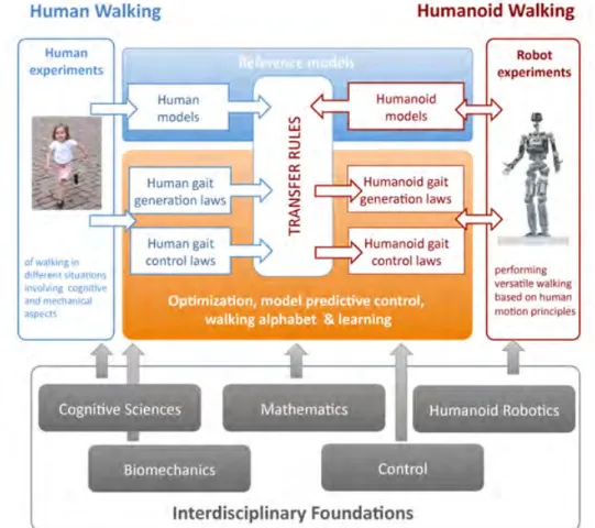
Figure 1: Graphical representation of the scientific approach of the KoroiBot project.

Context

This thesis has been written in the context of the European project KoroiBot (http://www. koroibot.eu/). The goal of the KoroiBot project is to enhance the ability of humanoid robots to walk in a dynamic and versatile way, and to bring them closer to human capabilities. As depicted in Fig. 1, the KoroiBot project partners have to study human motions and use this knowledge to control humanoid robots via optimal control methods. Human motions are recorded with motion capture systems and stored in an open source data bank which can be found at https://koroibot-motion-database.humanoids.kit.edu/. With these data several possibilities are exploited. Assuming that humans minimize some criteria we can use inverse optimal control methods to find those criteria. Walking alphabet and learning method [Mandery 2016] are also used to transfer human behaviors to robots. Finally, optimal control is used to build controllers that can eventually use these learned human behaviors while ensuring the robot safety. Research and innovation works in KoroiBot mainly target novel motion control methods for existing hardware. It also derives optimized design principles for next robot generations.

(12)

S

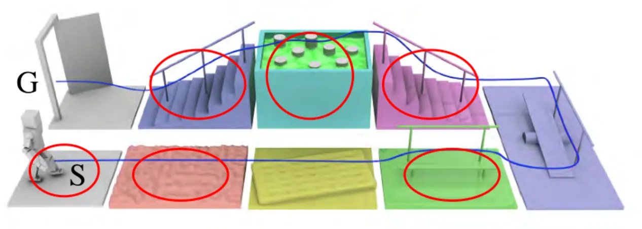
G

Figure 2: Challenges of the KoroiBot project. In red the challenges chosen by the LAAS-CNRS.

KoroiBot and robot challenges

In addition to this ambitious scientific aspect of the project, there is an important technical component. Following the blue line in Fig. 2, the different challenges of the project are to make humanoid robots:

walking on a flat ground, walking on an uneven ground, walking on a mattress,

walking on a beam with/without handrail, walking on a seesaw with/without handrail, climbing a stair case with/without handrail, walking on stepping stones,

going down a stair case with/without handrail, and walking through a door.

All the team owning a robot has to perform some of these challenges. In Fig. 3 we can see all the robot hosted by different partners. Ideally, the algorithms developed in the frame of the KoroiBot project has to be integrated on all the robots. In practice the partners chose parts of the challenge to be realized on their different robotic platforms

KoroiBot Key Performance Indicator (KPI)

In the European project KoroiBot we need to evaluate the improvement in terms of robot control and human likeness. In this context and in collaboration with the H2R project, a detailed set of key performance indicators (KPI) have been proposed [Torricelli 2015]. These KPI try to capture all the bipedal locomotion patterns.

A set of specific sub-function of the global motor behavior is analyzed (see Fig. 4). The different sub-function are divided in two. First, the sub-function associated to body posture task with no locomotion. And second the same sub-function but including the robot body transport. The initial condition may vary depending on the experiment to perform. This is the idea of the

(13)

5

Figure 3: List of the humanoid robot used in the KoroiBot project.

intertrial variability. For example standing still on a horizontal flat surface is easy to reproduce at will. Hence there is no intertrial variability. On the contrary, while doing push recovery, it is difficult to reproduce the exact same push several times. The sub-function are also classified taking into account the changes in the environment or not.

Each of these functions can be evaluated for different robots using the criteria depicted in Fig. 5. The performance are classified in two sub categories, quantitative performance and human likeness. In addition there are indications on the last two columns if the criteria is applicable on a standing task or on a locomotion task.

All the partners owning a humanoid robot need to perform an evaluation of these KPI. However some movement are not possible yet on some robots of the consortium. Hence, the different team picked meaningful criteria considering the current state of their robot and controllers.

The work done in the KoroiBot context

In LAAS-CNRS, the Gepetto team own the HRP-2 and the Romeo robots depicted respectively as the second and fourth robot in Fig. 3 from the left to the right. The Romeo robot is the

(14)

Figure 4: The motor skills considered in the benchmarking scheme. This scheme is limited to bipedal loco-motion skills. The concept of intertrial variability is analogous to the concept of unexpected disturbances.

(15)

7

Figure 5: The motor abilities and related benchmarks are classified in two categories: performance and human likeness. The performance category includes all those abilities related to stability (ability of maintaining equilibrium) and efficiency. The human likeness category includes all those abilities related to typical human behavior, under the perspective of kinematics and dynamics. For each ability, a specific benchmark has been identified. The last column specifies in what classes of motor skills (i.e., the function category of Fig. 4) the corresponding benchmark is applicable.

(16)

first human size prototype of Softbank Robotics and has very limited locomotion capabilities. Therefore I was in charge of integrating our algorithms on the HRP-2 robot. Among the challenges from Fig. 2 we picked the one with a red circle, i.e:

walking on a flat ground, walking on an uneven ground,

walking on a beam with/without handrail, climbing a stair case with/without handrail, walking on stepping stones,

and going down a stair case with/without handrail.

In addition to those challenges we added the perturbation rejection. At the beginning of the project we evaluated the KPI on the HRP-2 robot. In our case, we picked the KPI sub-functions meaningful considering the above selected challenges:

horizontal ground at constant speed, stairs,

soft terrain with constant compliance,

bearing constant weight (the robot’s own weight). Coupled with the following benchmarks:

success rate across N different trials, specific energy cost of transport, specific mechanical cost of transport,

All these choices are shown in the tables from Fig. 4 and Fig. 5 by red ellipses. The mathematical details and results are presented below in section "KoroiBot Key Performance Indicator (KPI)".

Reactive walking The results pointed out some interesting points. First the ground walking

velocity and versatility of HRP-2 can be improved. In this context we did a collaboration, presented in Chap. 1, with our mathematician colleagues from the University of Heidelberg. This collaboration leads to a new real time walking pattern generator with increased functionalities like obstacle avoidance. In addition to this, the implementation of the dynamic filter, presented by Nishiwaki and al. in [Nishiwaki 2009], increase the range of the reachable CoM velocity.

Multicontact motion generation The second problem that arose from the KPI was the

energy consumption during the stair climbing. One possible way for solving this problem is to distribute the robot weight over multiple contacts. Hence, we designed an innovative multi-contact controller to allow generic locomotion and the use of a handrail. Chap. 2 explains this contribution in details.

Fire hose manipulation The second application concerns perturbation rejection and has

been done in a collaboration with the Japanese national institute of Advanced Industrial Science and Technology (AIST). This application is inspired from the DARPA robotic challenge. The idea of this work is to see if a humanoid robot with average power and size like HRP-2 is able, using a state of the art controller, to pull a stiff fire hose. The details of the experiment are written in Chap. 3

(17)

9

One third power law In the frame of the KoroiBot project, researchers studied the human

motion to extract quantitative data. In fact they noticed that humans adapt their velocities in function of the curvature of their trajectories. The scientific question that we tried to answer is the following: "Can this law extracted from human motion help humanoid robots to walk ?" A fruitful collaboration with these experts allowed us to answer this question. This resulted in the design of an innovating controller for tracking cyclic trajectories of the center of mass. Chap. 4 present this work in details.

Human motion primitives and model predictive control Another collaboration with

human motion experts was done to study if motion primitives extracted from human behavior could be applied to humanoid robot. To answer this question we propose a whole body controller using upper body movement primitives extracted from human behavior and lower body movement computed by a walking pattern generator. Chap. 5 show these fused bottom up and top down approaches.

Reactive controllers In this thesis we studied reactive behavior for humanoid robot. We

designed applications that make the robot facing real case scenarios. The first application was done in the frame of a collaboration with Airbus/Future of Aircraft Factory. The idea was to build controllers for test case scenarios and evaluate if humanoid robot could go in a factory. We used online planner for obstacle avoidance, visual servoing coupled with a walking pattern generator to place the robot in a desired position, a whole body controller for screwing tasks, and center of pressure based walking pattern generator to climb stairs. Chap. 6 explains this contribution in details.

Problem statement and state of the art

Problem Statement

Robot behavior realization can be formalized using mathematical optimization. Considering a robot with N degrees of freedom, q a vector of information on its internal parameters and the environment v ∈ Rm_{. For a given behavior let us assume that it exists a function}

f(q, v, t) : Rn×m+1→[0, 1] such as it is equal to 0 when the behavior is realized. The problem amount to find a trajectory q(t) such that

minimize f(q, v, t) (1)

subject to g(q, v, t) < 0

h(q, v, t) = 0

with g being unilateral constraint an h bilateral constraints.

A common approach in robotics is to build an approximation ˆf of f. It depends on the

estimated current state of the environment ˆv(t), and an estimation of the current state of the robot in this environment ˆq(t). The formulations of ˆv(t) and ˆq(t) are injected in (1) to solve the optimization problem. In this document we will not address the problem of building ˆv but assume that an appropriate software module is providing the necessary information. Therefore

(18)

we will assume that a geometric description of the environment is available, and that a system is able to give a sufficiently accurate position of the robot in this environment. Practically this is done through a motion capture system. In the following we will present the formulation of (1) for the locomotion problem.

The locomotion generic optimal control problem

The state of the problem x is usually composed of the robot whole body configuration coupled with the whole body velocity. Let us now denote by q the whole body configuration and by ˙q the whole body velocity. The future contact point can be precomputed by a planner or included in the state of the problem. The control of this system u, can be the next derivative of the state, i.e ¨q, or the contact wrench φ =h

f_k τk

iT

with k ∈ {0, . . . , K}, K being the number of contact. Or the motor torques T. We denote by x and u the state and control trajectories.

The main idea here is to be able to compute joint trajectories satisfying the general equation of the dynamics, the initial and terminal constraints, and keeping balance. The following optimal control problem (OCP) represents a generic form of the locomotion problem:

min_{x, u} XS s=1 Z ts+∆ts ts `s(x, u) dt (2a) s.t. ∀t ˙x = dyn(x, u) (2b) ∀t φ ∈ K (2c) ∀t x ∈ Bx (2d) ∀t u ∈ Bu (2e) x(0) = x0 (2f) x(T ) ∈ X∗ (2g)

where ts+1 = ts+ ∆ts is the start time of the phase s (with t0 = 0 and tS = T ). Constraint

(2b) makes sure that the motion is dynamically consistent. Constraint (2c) enforces balance with respect to the contact model. Constraints (2d) and (2e) imposes some bounds on the state and the control. Constraint (2f) imposes the trajectory to start from a given state (typically estimated by the sensor of the real robot). Constraint (2g) typically imposes the terminal state to be viable [Wieber 2008]. The cost (2a) is typically decoupled `s(x, u) = `x(x) + `u(u)

whose parameters may vary depending on the phase. `x is generally used to regularize and

to smooth the state trajectory while `u tends to minimize the forces, then producing a more

dynamic movement. The resulting control is stable as soon as `x comprehends the L-2 norm of

one time derivative of the robot center of mass (CoM) denoted by c, [Wieber 2015]. Problem (2) is a difficult problem to solve in its generic form. And specifically (2b) is a challenging constraint. Most of the time the shape of the problem varies from one solver to another only on the formulation of this constraint. Hence, in the next section we will describe this equation in more details.

(19)

11

Robot dynamics

In this section we will present the instantaneous dynamics of a poly-articulated rigid system based on [Orin 2013] and [Kajita 2003b]. We will then present some humanoid robotics specific formulation.

General formulation of a robot dynamic

In general the Lagrangian dynamics of a robot is expressed :

M(q)¨q + C(q, ˙q) ˙q + G(q) = STT+ K X k=1 JT_k(q)   f_k τk   (3) with q =h x θ ˆq iT

, ˙q, and ¨q being the generalized state of the robot of size Rdim(SE(3))+N

and its derivatives, and N being the number of actuated joints of the system. Lets assume that dim(SE(3)) = 6 to consider 3 translation and 3 rotations. It is composed by the free flyer position x and orientation θ which is the position of an arbitrary joint position and orientation in the ground frame, typically the center of the robot pelvis. ˆq is the configuration vector of the joints. The matrix M ∈ R(6+N )×(6+N ) _{is the generalized inertia matrix described in}

[Wieber 2005] and [Sherikov 2016]. C models the centrifugal and Coriolis effects, G is the action of the gravity field, S = [0N ×6 IN ×N] is a matrix selecting the joint torques T. JT_k(q) is the

contact Jacobian, fk and τk are the forces and torques applied at the contact k. The first 6

equations of Eq. 3 correspond to the Newton-Euler equations.

Underactuated dynamics and centroidal momentum

In [Orin 2013], the above equations are reformulated to express the centroidal momentum dynamics :

h_G = A_G(q) ˙q (4)

with hG = [K L]T∈ R6 being the spatial momentum composed by the linear momentum

K and the angular one L. A_G is the first six lines of the inertia matrix M. If we express the time derivative of the robot total momentum expressed at the center of mass (4) we get the first six lines of (3): ˙K = m¨c =XK k=1 0_R kfk+ mg (5) ˙L =XK k=1 (pk− c) × 0Rkfk+ τk (6)

with again fk being the forces expressed at the contact point in the contact frame, 0Rk the

rotation matrix between the contact frame and the inertia frame, pk the contact point position,

(20)

m(¨c − g) = K X k=1 0_R kfk (7) mc ×(¨c − g) + ˙L = K X k=1 pk×0Rkfk+ τk (8)

This formulation shows that the dynamics of a poly-articulated robot can be reduced into its center of mass. The influence of each body on the center of mass is express through the term ˙L. This term express the influence of the translation and rotation of each body on the center of mass dynamics.

The control horizon

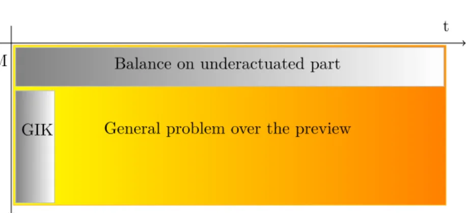
The equations expressed in Eq. 3 are expressed instantaneously. However controlling a robot dynamical movement needs anticipation due to the inertia. A control can be instantaneously satisfactory at time t, but not at time t + ∆t because of the presence of an obstacle for example. Imagine a car moving at constant speed (70 km h−1_{) with an instantaneous controller. This}

controller will not take into account that in few second the car needs to do a 90 deg turn. So when the turn comes the car has exactly ∆t seconds to react. Obviously the car will crash. On the contrary a human driver will anticipate the turn and slow down the vehicle before turning. That is the reason why anticipation and future prediction is needed. The inconvenient is that the complexity of the problem is equal to number of freedom multiply by the horizon size. Typically, HRP-2 has 36 degrees of freedom and we use a preview duration of 1.6 s (360) which gives 12960 free variables. This kind of problem cannot be solved yet in 5 ms with limited computational resources (see Fig. 6). The vertical axis corresponds to the instantaneous problem and the horizontal one show the size of the predicted future. In the following section we will present the optimal control problem for the locomotion of humanoid robot that researchers need to solve.

In the following we list some of the main algorithms solving (2) and show how they correspond to some specific choices of the generic template.

State of the Art

Hybrid controls

Other approaches exists for making robots walk on two legs. Historically passive walkers aims at achieving long walking behavior with a low energy footprint. This is realized through mechanical storage systems such as springs (DURUS [Reher 2016]), and efficient transmissions. In general the control approach tries to consider mainly the centroidal dynamics and uses stability criteria such as the Lyapunov criteria or the Poincaré map. They are less computationally expensive than optimal control methods. It has been shown in [Razavi 2015] that a stability criteria can be found using the method of Poincaré on the centroidal momentum. The authors were then able to implement an efficient controller law from this stability criteria. The work proposed by [Kaddar 2015] shows how to generate whole body dynamical motion using the same approach but using the whole body dynamic.

(21)

13

Those controllers are less expensive than optimal control because they required 1 control per phase. Typically for walking on flat floor, 2 phases are taken into account: single support and double support phase. On the contrary, optimal control methods need to discretize the dynamics and then to compute one control variable for each discretization step. Classically for walking 8 control variables needs to be computed for one step.

For standard walking the hybrid control is a good method [Westervelt 2007]. In fact, in free space with infinite flat ground walking motions can be considered as cyclic. Periodic phase and dynamics can be extracted from the Newton-Euler equations and in particular from the centroidal momentum.

One major difficulty is that aperiodic gate are complicated to manage as it would need a large number of controllers to drive the robot. Walking on uneven ground and maneuvering around an obstacles are typical case where the gait is aperiodic [Grizzle 2010]. In this thesis we will have to handle such cases like going through stepping stones or maneuver around obstacles, etc.

One major advantage of this method is that discontinuous phenomena, like impacts when the lands, are easily modeled using hybrid control. The impacts can then be manage by the controller after they occur. In the case of optimal control method it is rather expensive to include such phenomena. However in the context of the KoroiBotproject the motion we generated are not dynamical enough to consider huge impacts. To handle the foot landing we design sufficiently smooth trajectories to not provoke this kind of discontinuities in the robot states. Typically the foot trajectory ends with zero acceleration and velocity. Moreover, on HRP-2 specifically, there is a closed loop stabilizer which avoid perturbations and fit at best the smooth trajectories. Hence in this thesis we will focus on using optimal control methods.

Whole body formulations

t CoM

ˆ q

Balance on underactuated part

GIK General problem over the preview

Figure 6: Classical approach (in gray) organization vs. a more global handling of the problem

[Todorov 2014]

Fig. 6 depicts the classical approaches used so far. Indeed the full problem is nonlinear and has around 10 thousand variables and is represented by the whole rectangle. To be able to solve it researchers used heavy framework for nonlinear optimization. In fact in [Koch 2014] the authors implemented the above OCP and generated trajectories for the HRP-2 robot. The software used in this context computes multiple shooting method to solve nonlinear problems. The solution obtained was a smooth trajectory that allow a HRP-2 robot to step over a 20 cm

(22)

high obstacle. The experiment has been done in LAAS-CNRS. This motion is, for now in LAAS-CNRS, the record in terms of obstacle height. The bottom heck of this approach is the computation time. These trajectories took several ours to be computed. Another formulation implement the complete problem but use simplifications in the contact model. In [Tassa 2014] the authors uses Differential Dynamic Programming (DDP) to solve the problem. This is a very efficient way to compute a solution. However the current contact model is a spring and damper model. It produce good enough contact forces to perform multicontact reaching. However no walking could be performed as the the model provides none dynamically consistent force. An implementation of this software has been used with HRP-2 in [Koenemann 2015]. The solver was installed in a remote computer as it still needs multiple powerful CPUs to be used online. In [Koenemann 2015] the authors used a off board non-real-time Windows on a 12-core 4GHz CPU that computes the DDP under 100 ms. The PID controller of the robot runs on an embedded computer using a real time linux with a 2.93 GHz CPU. The connection between the two computer is done via wifi.

To summarize this, there are not yet powerful techniques that can be used with limited time and computational resources. As a consequence researchers try to simplify the problem. The next paragraph presents these approaches.

Mixed formulation

One simplification consist in taking into account the future of the under-actuated part of the dynamic plus the whole body instantaneous dynamics. In Fig. 6 this would correspond to the two gray areas but fused together.

During the DARPA robotics challenge the authors of [Kuindersma 2014] used a custom active set solver for quadratic programming to solve a mixed formulation. For the under-actuated formulation they used the seminal work of Kajita [Kajita 2003a]. In addition they used linearized friction cones and optimized the robot joint accelerations.

A recent thesis [Sherikov 2016] pursue this work of integrating under-actuated preview control inside a instantaneous whole body controller. The main difference between Sherikov and Kuindersma’s work is the under-actuated model predictive control used. In fact the walking task of the Sherikov’s framework is able to automatically find the foot steps following the formalism of [Herdt 2010a]. In Kuindersma’s framework the foot steps are precomputed by a planner.

Walking patterns in 3D

From this subsection on, the hypothesis of separating the under-actuated and whole body motion is made. The hypothesis is most used in the literature and correspond to the two separated gray rectangles in Fig. 6. This means that trajectories for the CoM, the free flyer and the end effectors are computed first. And only afterward the whole body control is deduced from these preliminary calculations. The work presented in this section are locomotion algorithm allowing multiple contacts.

An iterative scheme is proposed in [Hirukawa 2007] that can be written as an implicit optimization scheme whose cost function is the distance to a given CoM trajectory and given forces distributions. The resulting forces satisfies (2c) by construction of the solution. There is no condition on the angular momentum (6) neither on the viability of the final state (2g),

(23)

15

however the reference trajectory enforced by the cost function is very likely to play the same role.

In [Qiu 2011], (2c) is explicitly handled (using the classic linear approximation of the quadratic cones). As in [Perrin 2015], (2g) is indirectly handled by minimizing the jerk. No condition on the angular momentum (6) is considered. Additionally, the proposed cost function maximizes the robustness of the computed forces φ and minimizes the execution time. Finally, constraints are added to represent the limitation of the robot kinematics.

In [Perrin 2015], ˙L is null by construction of the solution. Moreover, (2c) is supposed to always hold by hypothesis and is not checked, while (2g) is not considered but tends to be enforced by minimizing the norm of the jerk of the CoM, like in [Kajita 2003a]. These assumptions result in an (bilinear)-constrained quadratic program that is solved by a dedicated numerical method.

In [Rotella 2015], (2c) is handled under a simple closed form solution, while (2g) is not considered. To stabilize the resolution, the cost function tends to stay close to an initial trajectory of both the CoM and the angular momentum, computed beforehand from a kinematic path. Consequently, (6) is not considered either (as it will simply stay close to the initial guess).

Walking patterns in 2D

In addition to the previous remarks, another difficulty is the bilinear form of the dynamics (8). When the contacts are all taken on a same plane, a clever reformulation of the dynamics makes it linear [Kajita 2003a], by neglecting the dynamics of both the CoM altitude and the angular momentum. In that case, (8) boils down to the constraint of the center of pressure point (CoP) to be in the support polygon.

Kajita et al. [Kajita 2003a] did not explicitly check the constraint (2c). In exchange, `u is

used to keep the control trajectory close to a reference trajectory provided a priori. Similarly, (2g) is not checked either. In exchange, `x tends to stabilize the robot at the end of the trajectory by

minimizing the jerk of the CoM. These three simplifications turns (2) into a simple unconstrained problem of linear-quadratic regulation that is implicitly solved by integrating the corresponding Riccati equation. Interesting motions can be perform using this walking pattern generator. [Evrard 2009] shows that tele-cooperation was possible using humanoid robot and teh walking pattern generator from [Kajita 2003a].

The LQR was reformulated into an explicit OCP [Herdt 2010b], directly solved as quadratic program. The OCP formulation makes possible the formulation of inequality constraints. (2c) is then explicitly checked under its CoP form.

A modification of this OCP is proposed in [Sherikov 2014] where (2g) is nicely approximated by the capturability constraint, which is a linear constraint on the CoM and its first time derivative in case of 2D contacts.

Computing the contact placements

When considering an explicit OCP formulation, additional static variables can be added to the problem. Typically, the placement of the contact, that are given as invariant in (2), might be computed at the same time. This was first proposed in [Herdt 2010b] for a 2D WPG, and similarly used in [Sherikov 2014] and other works by the same authors. Similarly, it was proposed in [Rotella 2015] to include it in the proposed 3D WPG, but this feature was not implemented

(24)

nor demonstrated. In both cases, the placements of the contacts are unlimited (or similarly limited to a convex compact set). The problem becomes much harder when the contacts might be taken among a discrete set of placements. In [Deits 2014], the problem was formulated has a mixed-integer program (i.e. having both continuous and discrete variables) in case of flat contact, and solved using an interior-point solver to handle the discrete constraints. In [Mordatch 2012], the same problem is handled using a dedicated solver relying on a continuation heuristic, and demonstrated for animating the motion of virtual avatars.

This is not an exhaustive bibliography. Many papers need to be cited but also replaced in their scientific context. So for sake of clarity, a more detailed bibliography is written at the beginning of each chapter. This allow a better understanding on the state-of-art which is specific to each chapter of this thesis.

KoroiBot Key Performance Indicator (KPI)

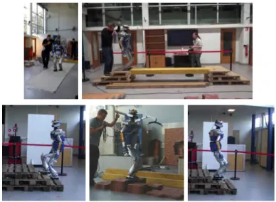
Figure 7: Sample of the experimental setup of the KoroiBot project in LAAS-CNRS

In the KoroiBot project we used key performance indicators (KPI) to analyze the behavior of the robot at the beginning and at the end of the project. These results lead us toward the improvements to be made. In 2013 the algorithm mostly used and implemented on HRP-2 in LAAS-CNRS where the walking pattern generators described in [Morisawa 2007] and in [Herdt 2010a]. The performance indicators chosen were:

the execution time TM,

the time to compute the motion Tthink,

the total energy consumed during a walking distance D,

Ewalk= Z tend tbbegin τ ωdt+ Z tend tbbegin Rk_c2τ2dt , E˜walk = Ewalk/D

with Ewalkbeing the total energy consumed counting the integral over time of the mechanical

(25)

17

joint torques and velocities, and R with kc being respectively the motor resistances and

torque constants.

the mechanical energy consumed during a walking distance D,

Emeca =

Z tend

tbegin

τ ωdt , E˜meca= Emeca/D

with Emeca being the integral over time of the mechanical power,

the deviation from the planned trajectory PTr, and the maximum speed reached Vmax.

The trajectories were generated offline and repeatedly played on the robot to analyze their robustness. Samples of the experimental setups can be seen in Fig. 7.

Straight walking

TM Tthink E˜walk E˜meca PTθr P

x

Tr P

y

Tr Vmax

7 s 2 s 47250 J/m 47070 J/m −0.0013 rad 0.026 m 0.052 m 0.125 m/s

From these results we can observe that the HRP-2 is very repeatable. However the room for improvement lies in the maximum velocity speed which is quiet slow.

3D walking

Here 3D walking means walking on flat ground but possibly a different height, like stair case or stepping stones. The walking pattern generators [Morisawa 2007, Herdt 2010a] normally does not allow the possibility to perform movement such as climbing stairs. For this reason we designed smooth feet 3D trajectories using B-Splines and a prior knowledge of the environment. Empirically we found trajectories that fits kinematics and dynamics constraints. The results of these implementation is shown in [Naveau 2014]

Walking in stairs or on stepping stones

TM Tthink E˜walk E˜meca PTr Vmax

7 s 2 s 256150, J/m 255270 J/m -

-This results shows the KPI value when the robot goes up the stair case. The important consumption of energy during the climbing up stairs is to be noted. Diminishing this power consumption is an important factor as it will decrease the loss of electrical energy and the mechanical stress on the robot. The repeatability of this experiment is around 40 %.

The results of the KPI, when the robot goes downstairs, are very similar to the going up experiment. The repeatability of the going down stairs motion is around 95 %. The only point is that the global energy is twice lower than when the robot is going up. The reason is that it is less fighting the gravity while going down.

For the stepping stone experiment the KPI were also very similar to the above two experiments. Though, as expected, the energy consumption is between going up and going down stairs. The repeatability of this experiment is around 50 %.

(26)

Walking on a beam

The major problem of this experiment is its success rate which is around 20 %. In order to improve this rate we need to take care of the robot balance and the robot feet placement. Indeed the two main reasons of the robot fall were the default of balance on the beam and the drift which is important as the beam length is 3 m long.

Step over obstacles

This manipulation has not been performed in the frame of this thesis. It is a work published in [Koch 2014] already presented in the above sections. The improvement to be made here is on the computation time. As explained before in subsection "Whole body formulations", these trajectory took several hours to be computed.

Contributions

The scientific contributions of my thesis are :

the design a novel real time walking pattern generator using nonlinear model predictive control (Chap. 1),

the implementation of two multicontact pattern generators using the centroidal dynamics. They both take the contact placements as input and produce dynamically stable center of mass (CoM) motion (Chap. 2).

In the context of the KoroiBot project several technical contributions are to be noted: the integration of a hose manipulation by HRP-2. The robot pick the hose from the floor and pull it to a desired position without falling,

the inclusion of the one third power law as control law for humanoid walking,

the elaboration of transfer rules to use upper body human motions integrated with a walking pattern generator (Chap. 5),

the study of potential application for humanoid robots in an industrial environment (Chap. 6) including,

the use of fast planning in order to make HRP-2 walking towards a desired position while avoiding obstacles,

the integration of visual servoing to track a target position while walking,

the use of the whole body motion generator (Stack-of-Tasks) to evaluate the kinematic feasibility of screwing motions,

the design of feet 3D trajectory to allow the robot to climb stairs or go across stepping stones and beams,

(27)

19

Publications

Journal

Accepted

• M. Naveau, M. Kudruss, O. Stasse, C. Kirches, K. Mombaur and P. Soueres. A Reactive

Walking Pattern Generator Based on Nonlinear Model Predictive Control. Robotics and

Automation Letters, 2017

Under revision

• A. Mukovskiy, C. Vassallo, M. Naveau, O. Stasse, P. Souères and M. A. Giese. Learning

Movement Primitives for the Humanoid Robot HRP2, 2016. (Submitted)

• A. Orthey, V. Ivan, M. Naveau, Y. Yang, O. Stasse and S. Vijayakumar. Homotopic

particle motion planning for humanoid robotics. 2015. (Submitted)

Conference

Published

• M. Karklinsky, M. Naveau, A. Mukovskiy, O. Stasse, T. Flash and P. Soueres. Robust

human-inspired power law trajectories for humanoid HRP-2 robot. In Int. Conf. on

Biomedical Robotics and Biomechatronics, 2016

• J. Carpentier, S. Tonneau, M. Naveau, O. Stasse and N. Mansard. A Versatile and Efficient

Pattern Generator for Generalized Legged Locomotion. In Int. Conf. on Robotics and

Automation, 2015

• M. Kudruss, M. Naveau, O. Stasse, N. Mansard, C. Kirches, P. Soueres and K. Mombaur.

Optimal Control for Multi-Contact, Whole-Body Motion Generation using Center-of-Mass Dynamics for Multi-Contact Situations. In Int. Conf. on Humanoid Robotics, 2015

• M. Naveau, J. Carpentier, S. Barthelemy, O. Stasse and P. Soueres. METAPOD - Template

META-PrOgramming applied to Dynamics: CoP-CoM trajectories filtering. In Int. Conf.

on Humanoid Robotics, 2014

• O. Stasse, A. Orthey, F. Morsillo, M. Geisert, N. Mansard, M. Naveau and C. Vassallo.

Airbus/Future of Aircraft Factory, HRP-2 as Universal Worker Proof of Concept. In

IEEE/RAS International Conference on Humanoid Robot (ICHR), 2014

Submitted

• I. G. Ramirez-Alpizar, M. Naveau, C. Benazeth, O. Stasse, J.-P. Laumond, K. Harada and E. Yoshida. Motion Generation for Pulling a Fire Hose by a Humanoid Robot, 2016. (Submitted)

(28)

(29)

Chapter 1

(30)

(31)

1.1. Introduction 23

In the present chapter we present a real-time nonlinear model predictive control (NMPC) executable on the humanoid robot HRP-2. This chapter has been developed in the frame of the collaborative project KoroiBot and published in [Naveau 2017]. Following the idea of “walking without thinking", we propose a walking pattern generator that takes into account simultaneously the position and orientation of the feet. A requirement for an application in real-world scenarios is the avoidance of obstacles. Therefore, an extension of the pattern generator that directly considers the avoidance of obstacles is derived. The algorithm uses the whole-body dynamics to correct the center of mass trajectory of the underlying simplified model. The pattern generator runs in real-time on the embedded hardware of the humanoid robot HRP-2 and experiments demonstrate the increase in performance with the correction.

In Sec. 1.1.1 we present the motivation and the related works. Sec. 1.2 is a reminder of the LIPM equation as well as the principles used in [Herdt 2010a]. Sec. 1.3 depicts the formulation of the problem as a sequence of locally linearized quadratic problems and the real-time feasible solution by applying the idea of the so called "real-time" iteration. A particular treatment of the dynamical filter is given in Sec. 1.4. Finally, our practical contribution, showing that the algorithm can be implemented in real-time on the humanoid robot HRP-2, is detailed in Sec. 1.5.

1.1 Introduction

1.1.1 Motivation

The recent DARPA robotics challenge have shown the need for humanoid robots with an increased level of functionality enabled by proper control. Such complex robots must provide a simple interface for humans and handle as much as possible the motion generation autonomously. A general scheme is to use a motion planner to find an optimal path over a discrete set of step transitions between two quasi-static poses [Chestnutt 2010, Hornung 2012]. The foot-steps transition are given by a statistical exploration of a whole-body controller together with a walking pattern generator. The planner then finds a feasible sequence of quasi-static poses and foot-step transitions which minimizes a cost function and avoids obstacles. This solution is then improved online while ensuring feasibility, see for instance [Perrin 2012]. In general it is not possible to realize real-time motion planning by directly using the controller itself because it is not possible to run more than one or two instances of the same controller before collision. Therefore, when the planner fails it is necessary to solve a continuous local problem which will provide a feasible solution different from the precomputed one [Chestnutt 2010]. The statistical exploration can be advantageously used to cast an optimization problem to find an initial guess [Chestnutt 2010]. Recently, Deits proposed to define the area of convergence for a local convex problem with linear constraints [Deits 2014] for a template model. With template models the inertia related to the whole-body motion is ignored, regulated to zero or corrected. In this chapter it is corrected by means of a dynamic filter. It is shown in the experimental section that it is drastically improving the performances over [Herdt 2010a] on the same robot. The use of template model is a practical solution on platforms with limited computation capabilities. Even if advanced whole-body motion controllers are now closer to real-time feasibility, e.g. the one proposed by Todorov which was recently applied to HRP-2 [Koenemann 2015], they still need powerful multi-core CPUs which limit their integration on humanoid robots due to heat and power consumption.

(32)

W x y z C x y z Safety Area vrefk

Figure 1.1: HRP-2 avoiding reactively on an obstacle, even if the reference velocity vref_k drives it into it.

The upper body geometry is taken into account by setting a constraint (in green) such that the robot is sufficiently away from the obstacle (in red).

Another improvement of this chapter over the method developed in [Herdt 2010a] is the nonlinear formulation which here allows to deal with obstacle. More precisely [Herdt 2010a] integrates the information provided by statistical exploration of the controller feasibility between two foot-step transitions. It makes possible to correct foot-steps while having a guarantee over their feasibility. It is realized by reformulating the optimization problem to generate balanced Center-of-Pressure (CoP) and Center-of-Mass (CoM) trajectories where the free variables are the jerk of the CoM as well as foot-step positions and orientations. The feasible foot-steps, i.e. free of self-collision and singularities, are specified through linear constraints. This works well for level ground walking, unfortunately integrating obstacles with linear constraints implies a pre-processing of the environment or to use a different solver.

The present chapter shows that obstacles can be dealt with in real-time using a nonlinear scheme. Although not demonstrated in this chapter, it can be coupled with a real-time planner. The proposed method would provide a local feasible solution while the planner is looking for a global feasible solution [Perrin 2012].

1.1.2 Related work

Previous works have proposed to apply Model Predictive Control (MPC) to humanoid robots walking by considering either the whole body or a template model. When a model is available for a robot, MPC has several advantages. It can be very fast when using analytical solutions [Morisawa 2007, Tedrake 2015, S. Faraji 2014]. However such formulation makes generally some specific assumptions to find the derivation. This makes difficult the extension to other walking functionalities. On the other hand MPC schemes formulated as an optimization problem with a finer discretization grid can be more easily modified to include various walking modes inside a single formulation [Sherikov 2014]. In addition MPC as an optimization problem is becoming increasingly popular [Feng 2013], because for a given class of problems it allows using efficient

(33)

1.1. Introduction 25

off-the-shelf solvers. Moreover several methods exist to increase the efficiency of solvers for NMPC problems. For instance, it is possible to use warm-starts or use a sub-optimal solution while maintaining feasibility [Boyd 2004]. The goal in humanoid robotics is to find a problem formulation which realizes all the needed functionalities and copes with the robot capabilities. The locomotion problems described in [Mordatch 2012], that include multi-contacts and consider the whole robot model over a time horizon, are not yet solvable in real-time and strongly depend on the models used to represent the physics.

Despite numerous efforts to address this large scale nonlinear problem with roughly ten thousand variables [Koenemann 2015, Dai 2014b], no solution yet exists to generate physically consistent controls in real-time using humanoid robot embedded computers. On the other hand template models projecting the overall robot dynamics to its CoM are used in research works [Wensing 2014, Orin 2012, Kajita 2003a, Englsberger 2015], and already showing promising performance. Motion generation with template models can sometimes be solved analytically, and in such cases provide fast solutions that are particularly well suited for platforms with limited computational power. However, when increased CPU power is available, MPC-based solutions with the whole model are much more complete and reliable. Furthermore, as they can be easily modified, they provide more adaptive functionalities. In this chapter, with a bottom-up approach, we are trying to increase the functional level of a control architecture that already works on an existing humanoid robot, HRP-2 [Herdt 2010a]. The point of this chapter is to present extensions of the linear MPC scheme presented in [Herdt 2010a], that allows automatic foot placement in real-time. For instance, the problem depicted in Fig. 1.1 shows the humanoid robot HRP-2 driven by a desired velocity provided by the user. The former scheme [Herdt 2010a] was specifically formulated as a cascade of two quadratic programs (QPs). Foot-step orientations are solution of the first problem, while the second solution of the second QP provides the CoM trajectory and foot-step positions. This separation is efficient because the constraints are linear. If an obstacle has to be taken into account then the constraints have the shape depicted in Fig. 1.2, which is not convex anymore. To maintain the convexity, the solution would be to pre-process the obstacle and the feasibility area of the foot-steps. However a linearization of the obstacle boundary is equivalent to adding a linear constraint as depicted in Fig. 1.2. The algorithm proposed in this chapter is doing a similar operation and therefore no pre-processing is necessary. This is one of the major contribution of this chapter in comparison to [Herdt 2010a]. The proposed nonlinear extension takes into account the exact expression of constraints such as, for instance, locally avoiding a convex obstacle. Other formulations for walking motion generation have already been proposed. [Deits 2014] is using mixed-integer convex optimization for planning foot-steps with Atlas. [Ibanez 2014] is using mixed-integer convex optimization for MPC control and foot steps timing. In this work we introduce three nonlinear inequalities to handle balance, foot step orientation and obstacle avoidance. This new real time walking pattern generator has been successfully tested on the humanoid robot HRP-2 as depicted in Fig. 1.1. A key ingredient for achieving real-time performance was the following observation:

one real-time iteration of the nonlinear scheme is enough to find a reasonable solution.

1.1.3 Contribution of the chapter

• It proposes a nonlinear reformulation of classical walking pattern generator able to find simultaneously foot-step positions and orientations.

(34)

additional linear constraint

Figure 1.2: Walkable zone distorted by a convex obstacle

• It introduces nonlinear constraints able to cope with obstacles in the environment. • It shows experimentally that one iteration of the nonlinear iterative scheme provides a

suboptimal but sufficient solution for practical cases.

• Thanks to the use of a dynamical filter that corrects the CoM trajectory to compensate the limitation of the template model as in [Nishiwaki 2009] the whole body dynamics can be taken into account. This technical implementation has a strong impact on the robot performances.

• The whole algorithm runs in real time on the embedded hardware of the human-size humanoid robot HRP-2.

To be completely fair we are not doing NMPC using sensor feedback on the walking pattern generator. The feedback loop of the algorithm is done by the dynamic filter (see Fig. 1.3). In fact the sensor feedback is already done by the commercial stabilizer from Kawada Industry. Additional ongoing work is done to close the loop but the stabilizer is a closed-source software. Hence it is rather difficult to be exactly sure of its behavior.

1.2 Derivation of the dynamics

In this work the well known Linear Inverted Pendulum Model (LIPM) from [Kajita 2003a] is used as the template model of the robot’s dynamics and the following assumptions are made: 1) the angular momentum produced by the rotations of all the robot parts is supposed to be zero, 2) the robot CoM evolves on a horizontal plane, 3) the normals of the contact forces have to be collinear. As a consequence, each quantity can be expressed as a function of three degrees of freedom (DoFs), which are the projection of the robot CoM (x, y)-position on the ground plane and its free-flyer orientation θ around the vertical axis z. The reader is kindly referred to [Herdt 2010a] for a detailed description of the several terms omitted for a sake of clarity in the following section.

1.2.1 Discretization of CoM dynamics

In order to obtain a smooth trajectory, one controls the robot CoM through its jerk ...cν _{on a}

preview horizon, where c denotes the position of the CoM in the world frame and ν ∈ {x, y} is used to simplify the notation. This is done by applying a constant sampling period T and by assuming a piecewise constant jerk on each interval, i.e. ...cν

k(t) ≡ constant, t ∈ [kT, (k + 1)T ],

(35)

1.2. Derivation of the dynamics 27

The following time-stepping scheme maps the current state of the frame cν

k to the future states by ˆcν k+j = Ajˆcνk + j−1 X i=0 AiB...cν_k+i , j ∈[0, N], (1.1) ˆcν k=     cν_k ˙cν k ¨cν k     , A=     1 T T2 /2 0 1 T 0 0 1     , B=     T3 /6 T2 /2 T     . (1.2)

To express the CoM over the preview horizon the vector Cν

k+1 of size RN and its derivatives are

defined as C_k+1ν =hcν_k+1 . . . c_k+Nν iT , ˙C_k+1ν =h˙cν k+1 . . . ˙cνk+N iT , ¨ C_k+1ν =h¨cν k+1 . . . ¨cνk+N iT , ...Cνk+1 = h... cν_k+1 . . . ...cν_k+NiT .

Using eq. (1.1), the above vectors can be expressed as a function of the initial state ˆcν k and

the CoM jerk ...Cνk+1. The latter belongs to the free-variable vector of the optimization problem

described in section 1.3.

1.2.2 Linear inverted pendulum dynamics

In this chapter the balance criteria used is the one that have the center of pressure (CoP) in the convex hull of the robot’s support polygon, which is defined by the contacts with the ground [Kajita 2003a] (see Sec. 1.3.3). Hence, the CoP has to be expressed in terms of the system’s free variables, i.e. the CoM jerk. Using the assumptions made in the introduction of Sec. 1.2, the robot CoP can be expressed as a linear function of the CoM, i.e.

zν_k+n=h1 0 −h_/ g

i

ˆcν

k+n, ν ∈ {x, y} , n ∈[0, N − 1],

with h = cz_{− z}z _{being the height of the CoM with respect to the ground and g the norm of the}

gravity vector. Using eq. (1.1), a recursive expression for the future evolution of the CoP for a fixed horizon of N sampling steps is given by

z_k+nν =h1 0 −h_/ g i " Anˆcν_k + n−1 X i=0 AiB...cν_k+i # . (1.3)

As in Sec. 1.2.1, the vector Zν k+1=

h

zν_k+1 . . . z_k+nν iT , of size RN, is used to describe the CoP

on the preview horizon. This vector can then be expressed in terms of ˆcν k and

...

Cνk+1.

1.2.3 Automatic foot step placement

The adaptive placement of the feet, with the aim to ensure balance of the robot even under external perturbations, is a key-feature of the algorithm. To this end, consider a frame F attached to the support foot, with its current position and orientation on the ground given by fη

(36)

denoted by

F_k+1η =hf_k+1η f_k+2η . . . f_k+Nη iT

F_k+1η = vk+1fkη+ Vk+1F˜k+1η (1.4)

with Fη

k+1 of size RN representing the foot support position at each time step and ˜F η

k+1 of size

Rnf _{the actual free variables of the problem. The vector v}

k+1∈RN and matrix Vk+1 ∈RN ×nf

indicate which step falls in which sampling interval (see [Herdt 2010a] for more details). Sampling times correspond to rows, steps to columns, and nf is the maximum number of double support phases in the preview.

In theory, the usage of a single point mass as model prevents the definition of an orientation. In [Herdt 2010a] a frame attached to the center mass is defined and the orientation of this frame and the feet directions are optimized. In this work only the foot step orientations are optimized, and the orientation of the robot free-flyer is computed from this solution. Let ffθ_{(t), f}θ,L_{(t) and}

fθ,R(t) be respectively the orientation of the free-flyer, the left foot and the right foot at any

time t. Hence ffθ_{(t) is by convention :}

    ffθ_(t) ˙ffθ (t) ¨ffθ (t)    =     1 2(fθ,L(t) + fθ,R(t)) 1 2( ˙f θ,L_{(t) + ˙f}θ,R_(t)) 1 2( ¨fθ,L(t) + ¨fθ,R(t))     .

1.3 Nonlinear Model Predictive Control

Solving the orientation problem separately from the position problem is a workaround to linearize the CoP (eq. (1.13)) and foot position (eq. (1.15)) constraints derived below. However, computing separately the orientation and then injecting the solution into the position QP amounts to solve a different problem than the nonlinear combination of both. In the following the nonlinear problem will be derived and analyzed, and an appropriate approach allowing the real-time execution of the algorithm on the robot will be proposed.

1.3.1 The controller Walking Pattern Generator Dynamic Filter Generalized Inverse Kinematics Robot Hardware Simulation/Robot V elref cref fref ˜cref fref qref ˙qref

Figure 1.3: The control scheme: V elref is the input velocity. cref _{and f}ref _{are respectively the CoM and}

the feet 3D trajectories ˜cref _{is the CoM trajectory filtered. q}ref_, _˙qref _{denote respectively the generalized}

coordinate vector and its derivation.

A scheme of the controller is shown in Fig. 1.3. This open-loop controller is used for tracking respectively a referenced linear and angular velocity. In the first step, the walking pattern generator (WPG) computes the foot steps and CoM jerk from the given velocity

(37)

1.3. Nonlinear Model Predictive Control 29

V el_k+1ref = hV elx,ref_k+1 V ely,ref_k+1 V elθ,ref_k+1 i. Then it uses an Euler integration scheme to compute

the CoM trajectory from its jerk and polynomials of fifth order to retrieve 3D trajectories for the feet from the foot step planning. The CoM computed by the WPG is then filtered (see Sec. 1.4) and sent altogether with the feet trajectory to a generalized inverse kinematics algorithm. The output is a whole-body walking trajectory that can be applied directly on the robot. The WPG is then reinitialized with the current reference velocity input and with the corrected initial states of the dynamic filter.

1.3.2 The cost function

The cost function used in the NMPC is given by min Uk α 2J1(Uk) + α 2J2(Uk) + β 2J3(Uk) + γ 2J4(Uk) (1.5)

with α, β and γ being the weights of the cost function and Uk the free variables of the problem

defined as U_kx,y= h_... Cxk F˜kx ... Cyk F˜ y k iT , Ukθ = ˜F θ k, Uk= h U_kx,y Uθ k iT . (1.6)

J1(Uk) is the cost function related to the linear velocity tracking

J1(Uk) = k ˙Ck+1x − V el x,ref k+1 k22+ k ˙C y k+1− V el y,ref k+1 k22.

J2(Uk) is the cost function related to the angular velocity tracking

J2(Uk) = kFk+1θ −

Z

V elθ,ref_k+1 dt k2₂.

Experiments have shown that a different weight between linear and angular velocities was not necessary at this stage. J3(Uk) is the cost function minimizing the distance between the CoP

and the projection of the ankle on the sole

J3(Uk) = kFk+1x − CoPk+1x k22+ kF

y

k+1− CoP y

k+1k22. (1.7)

J4(Uk) is the cost function minimizing the norm of the control

J4(Uk) = k

...

Cxk+1k22+ k

...

(38)

The above minimization function can then be express in a canonical form min Uk 1 2 UkT QkUk + pkT Uk, (1.8) with Qk=   Qx,y_k 0 0 Qθ k  , pk=   px,y_k pθ k  , Qθ_k= α Inf, pθ_k= α      h 1 . . . nfi TstepV elθ,refk+1 +      1 ... 1      f_kθ      .

The reader is kindly referred to [Herdt 2010a] for the defintion of Qx,y _{and p}x,y_{. The matrix Q}θ k

and pθ

k are derived because we use a slightly different method than [Herdt 2010a] to deal with

the orientation.

1.3.3 The constraints

First of all the balance of the robot has to be ensured, then the feasibility of the foot step needs to be verified. Finally, the nonlinear constraint which implements the obstacle avoidance is described. It is one of the contribution introduced by this chapter. The following exposition is based on [Herdt 2010a].

1.3.3.1 Balance constraint − →_x − →_y pz 1 pz 2 pz 3 pz4 Acop,Bcop θ

Figure 1.4: Shape of the foot with the position vector pz_i describing the support polygon and θ representing

its orientation. The4 × 2 matrix Acop and the 4 × 1 vector Bcop are the linear algebra representation of

the edges.

The CoP has to remain inside the support polygon [Wieber 2002]. This polygon is depicted in Fig. 1.4. The set of linear inequalities representing the convex polygon is denoted as Acop

and Bcop. Only one foot is modeled as a support polygon for two reasons: 1) HRP-2 feet are

symmetrical, 2) the sampling period of the problem is designed in a way that no iteration of the optimization problem falls into a double support phase. The CoP at instant k, (zk= [zkx z

y k]T),

(39)

1.3. Nonlinear Model Predictive Control 31

see Sec. 1.2.2) lies inside the support polygon if and only if

AcopR(fkθ) (zk− fk) ≤ Bcop (1.9)

h

Ax,θ_cop,k Ay,θ_cop,ki(zk− fk) ≤ Bcop (1.10)

R(f_kθ) =   cos(fθ k) sin(fkθ) −sin(fθ k) cos(fkθ)  , (1.11) where fk = [fkx f y k]T, A x,θ

cop,k is the left column of AcopR(fkθ) and A y,θ

cop,k is the right one. Using

eq. (1.4) the constraint for each time step of the preview horizon is defined by

Dk+1(Ukθ)   Z_k+1x − v_k+1f_kx− V_k+1F˜_k+1x Z_k+1y − v_k+1f_ky − V_k+1F˜_k+1y  ≤ bcop k+1 (1.12)

With bcop k+1= [Bcop. . . Bcop]T and Dk+1(U_kθ) =



   

Ax,θ_cop,k+1 0 Ay,θ_cop,k+1 0

... ...

0 Ax,θ_cop,k+N 0 Ay,θ_cop,k+N

     .

From eq. (1.12), the canonical form of the constraint is

Acop,k(Ukθ) U x,y

k ≤ Ucop,k, (1.13)

where Acop,k(Ukθ) is a matrix depending on Ukθ which makes this constraint nonlinear. And Ucop,k

is the upper bound vector. The last steps of the derivation are detailed in [Herdt 2010a].

− →_x − →_y Ar,Br Al,Bl Support Foot θ pl 1 pl₂ pl₃ pl₄ pl 5

Figure 1.5: Shape of the selected convex polygon boundary of the foot placement. The5 × 2 matrix Ar,l

(40)

1.3.3.2 Foot step feasibility constraint

This constraint uses the same convex hull as in [Herdt 2010a] to ensure the feasibility of the steps [Perrin 2010]. For HRP-2 this convex hull is shown in Fig. 1.5. The set of linear inequalities representing this convex polygon is defined by Af oot and Bf oot. Instead of r or l the lower index

f ootis used because the problem is symmetrical. The constraint, representing the fact that the

swing foot has to land inside the convex hull, is given as

Af ootR(θ)(fk+1− fk) ≤ Br,l. (1.14)

In the exact manner as in eq. (1.13), the vector and matrices depicted in Sec. 1.2 are used to express this constraint for each previewed foot step. More details are presented in [Herdt 2010a]. The canonical form of the constraint is

Af oot,k(Ukθ) U x,y

k ≤ Uf oot,k, (1.15)

where Af oot,k(Ukθ) depends on Ukθ like Acop,k(Ukθ), which makes this constraint nonlinear.

And Uf oot,k is the upper bound vector.

1.3.3.3 Foot orientation constraint

One additional feasibility constraint considers the maximum and minimum angle between both feet

− θ_thresh ≤ F_k+1θ − F_kθ ≤ θ_thresh, (1.16)

with the canonical form

Uθ,k ≤ AθUkθ ≤ Uθ,k (1.17) with : Aθ=          1 0 0 0 −1 1 ... ... 0 ... ... 0 ... 0 −1 1          , Uθ,k = h

θthresh+ fkθ θthresh . . . θthresh

iT , Uθ,k = h −θ_thresh+ fθ k −θthresh . . . −θthresh iT .

In practice the bound θthresh= 0.05rad takes into account the hardware limits. At this stage,

the optimization problem allows the robot to place its feet anywhere inside the convex hull at any moment. In [Herdt 2010a], the velocity of the foot is limited by bounding the feasible foot step area that corresponds to a maximum velocity. We chose to use the same idea extended to all the foot steps degrees of freedom. This significantly decreases the variation of accelerations before foot landing.