An efficient implicit approach for the thermomechanical
behavior of materials submitted to high strain rates
P.P. Jeunechamps
1– J.P. Ponthot
11
Université de Liège, LTAS-MC&T, Chemin des Chevreuils 1, B4000 Liège, Belgium,
ppjeunechamps@ulg.ac.be , jp.ponthot@ulg.ac.be
Abstract. In the present paper, three solutions are proposed to simulate fast phenomena with finite element
method at best. At first, material constitutive laws of Johnson-Cook and Zerilli-Armstrong types are implemented. These well-known laws are efficient for the description of material behavior at high velocities, especially for material used in automotive or aeronautics industry. The second contribution of this paper is the coupling of an implicit Chung-Hulbert algorithm taking into account the inertial effects with a staggered scheme for solving the thermal problem. The last input of this paper is the use of EAS (Enhanced Assumed Strain) finite elements to better capture complex strain modes, especially bending that is not accurately evaluated with classical finite elements. These EAS finite elements are used in the scope of thermomechanical dynamic phenomena implemented in a modular C++ environment at the University of Liège in the home made software METAFOR.
1. INTRODUCTION
In a finite element simulation of high strain rates phenomena, four main effects have to be taken into account. At first, adequate constitutive equations including strain rate and temperature effects must be used to measure the hardening due to the high strain rate and the thermal softening of the material. Secondly, the study of fast phenomena must be coupled with large strains formulation for which every modes of physical strains must be considered (in other words one has to avoid locking of the finite elements). Therefore, it is important to use finite elements providing a good answer to different loading modes, especially bending, with a reasonable CPU time. Thirdly, numerical solution algorithms have to accurately evaluate the temperature evolution during the process. Moreover, due to the fastness of the studied phenomena, the mechanical inertial effects can not be neglected and the resolution algorithms have to be able to quantify these dynamic effects. The last important point is a reasonable global CPU cost.
2. MATERIAL CONSTITUTIVE LAWS IN LARGE STRAIN AND HIGH STRAIN RATES
For the mathematical description of material behavior submitted to fast phenomena, the constitutive laws describing the evolution of the yield limit have to take into account the material hardening due to large strains, the viscosity effects due to the high strain rates and the thermal softening. Those requirements impose the constitutive laws to depend simultaneously on plastic strain, plastic strain rate and temperature in a thermomechanically coupled formulation.
In this paper, two constitutive laws are used. At first, the classical Johnson-Cook law (see [1]) which depends on the plastic strain; the strain rate and the temperature. This law has the form defined by (1):
(
)
1 2 2 0 0 1 ln ln 1 m n room vm melt room T T A B C C T T ε ε σ ε ε ε ⎛ ⎛ ⎞ ⎞⎛ ⎛ − ⎞ ⎞ ⎜ ⎟⎜ ⎟ = + + + ⎜ ⎟ −⎜ ⎟ ⎜ ⎝ ⎠ ⎟⎜ ⎝ − ⎠ ⎟ ⎝ ⎠⎝ ⎠ & & & & (1)where ε is the (scalar) equivalent plastic strain, ε& the strain rate and T the temperature. A, B, n, C1, 2
C ε&0, and m are the seven material parameters. The first term represents the isotropic hardening (power law), the second term is the viscosity factor (with a linear and non linear term according to the logarithmic strain rate) and the last one represents the thermal softening. Every parameter can depend explicitly on temperature. This law is a phenomenological one. It is used for strain rates around 1000 s-1. The second classical constitutive law is the Zerilli-Armstrong one (see [2]). It is written in general case as described in (2) for BCC metals and in (3) for FCC metals
(
)
1 0 2exp 3 4 ln 5 n vm C C T C T C σ =σ + − + ε& + ε (2)(
)
2 0 2 exp 3 4 ln n vm C C T C T σ =σ + ε − + ε& (3)where σ0
,
C2, C3, C4, C5, n1 and n2 are seven material parameters. Zerilli-Armstrong’s law isbased on the analysis of microstructural mechanisms such as grain size, crystal structure and dislocation mechanisms.
3. IMPLICIT THERMOCHANICAL ALGORITHM
When describing fast phenomena, it is important to take into account two effects. The first one is the inertial acceleration. If this inertial term is often neglected in metal forming problems, it becomes very important for an accurate description of fast phenomena. The second effect is the thermal softening due to plasticity. In a slow phenomenon, it can be neglected because heat production is limited and heat can be dissipated by conduction and exchange with external environment without much affecting the response. For fast processes, the increase in temperature can be high and is concentrated in areas of high strains because no conduction or exchange is possible within such a limited time. So a coupled thermomechanical numerical analysis taking into account these two effects is essential to solve accurately dynamics problems.
Usually, explicit methods are used for the resolution of such dynamic thermomechanical problems. The advantages of these methods are the ease of implementation and a low memory requirement but there are known to be slow because of numerical instabilities when time steps grow, especially in coupled simulations. Implicit method can be more efficient in CPU cost because these methods are unconditionally stable and large time steps can be used. But they are more difficult to implement and require more memory (stiffness matrix must be computed, stored and inverted at each iteration).
In this paper, the thermomechanical problem is solved thanks to an implicit staggered scheme (see [3-4]) that consists in the separation of the mechanical unknowns from the thermal ones. This method allows the reduction of the coupled system size. The total coupled system is split into a mechanical system and a thermal one:
' ' M M M MM MT M M TM TT T T T T T ⎧ = ⎛ ⎞⎛ ⎞ ⎛= ⎞ ⎪ → ⎨ ⎜ ⎟⎜ ⎟ ⎜ ⎟ = ⎪ ⎝ ⎠⎝ ⎠ ⎝ ⎠ ⎩ K q g K K q g K K q g K q g (4)
The coupling terms are included in thermal dependencies in the integration of material constitutive laws and in the heat equation resolution. The resolution of the coupled problem is achieved in two steps: at first a mechanical step to solve the mechanical problem (see (5)) and secondly a thermal step to solve heat equation (see (9))
For the resolution of mechanical problem, the Newmark algorithm family is selected (see [5-6]). At each time step, the mechanical system (5) has to be solved for each node:
0
, f ext int t ⎡t t ⎤
= − ∀ ∈ ⎣ ⎦
Mx&& F F (5)
With M the mass matrix, x&& the acceleration vector, Fext the vector of external forces and Fint the vector of internal forces. The evaluation of velocities and position is evaluated by the Newmark method (see [5]): 1 1 2 2 1 2 n+ = n+ Δt n+⎛ −β⎞Δt n+ Δβ t n+ ⎜ ⎟ ⎝ ⎠
x x x& &&x &&x (6)
(
)
1 1 1
n+ = n+ −γ Δt n+ Δγ t n+
x& x& x&& x&& (7)
Where x is the position vector, x& is the velocity vector, n is the current time step number (for which everything is known), n+1 the next time step, Δt the time step increment, β and γ are the Newmark parameters. This pure Newmark scheme is only conditionally stable. To become stable at least for linear problems, numerical dissipation is introduced by weighting accelerations and forces between time step n and time step n+1:
(
)
1(
)
(
1 1)
(
)
1 n n 1 n n n n
M M F ext int F ext int
α + α α + + α
− Mx&& + Mx&& = − F −F + F −F (8)
This method is known as Chung-Hulbert algorithm (see [7]). For an adequate choice of parameters M
α and α , this scheme can be proved to be unconditionally stable in the linear range. F
The thermal part of the coupled problem consists to the resolution of the heat equation (9) for each time step and each node:
{ 0,
irr s te f
Flux Sources
cT r W W W div t t t
ρ &=ρ + & − & + & − q ∀ ∈ ⎣⎡ ⎤⎦
144424443 (9)
where ρ is heat capacity, c ρ is volumic heat source, r irr vp
W& =σ ε& is irreversible stress power generated by (visco)plasticity, s
(
1)
irrW& = −β W& is the power stored in material for microstructural evolution, W&te
is thermoelastic dissipation and q is heat flux. This equation is solved at each time step by mid-point generalized or trapezoidal numerical scheme (see [4]).
The advantage using such implicit algorithms can be illustrated in the Taylor Bar problem. This well-known problem consists in the crushing of a cylindrical bar against a rigid wall. The bar has an initial velocity and the process stops when all the kinetic energy is dissipated. The experimental results, material and geometrical data are taken from [1]. Three materials were simulated: copper, iron and steel. The materials are modeled with Johnson-Cook’s law (1). Three impact velocities are used for each material. The problem is illustrated in Figure 1 where initial and final configurations are represented.
The different algorithms to solve the mechanical part of the problem can be easily compared on this example. All the algorithms give similar solutions but CPU time is very different when using different methods. Four algorithms were investigated: an explicit algorithm, the Newmark algorithm without numerical dissipation, the HHT algorithm (only the forces are weighted, i.e. α = ) and the M 0
Chung-Hulbert algorithm (with α = −M 0.97 and α =F 0.01. The results of comparison are illustrated in Figure 2. It can be seen that Newmark algorithm is the most expensive algorithm. The CPU time increases with initial velocity impact for the explicit algorithm (the stability limit decreases when velocity increases), while it remains more or less constant for implicit algorithms using numerical dissipation.
a) b)
Figure 1. Taylor bar simulation. a) Initial configuration; b) Final configuration
V0 = 197m/s V0 = 221m/s V0 = 279m/s 0 1 2 3 4 5 6 7 Initial velocity CPU t im e ( m in ) Explicit Newmark HHT Chung-Hulbert
Figure 2. Comparison of CPU time for explicit and implicit algorithms
4. ENHANCED ASSUMED STRAIN FINITE ELEMENT
Usual finite elements, such as Selective Reduced Integration (SRI) elements, as used in the previous paragraph are well-known to be robust, accurate and stable with a reasonable CPU-time cost. But they are subjected to locking when submitted to shear or bending dominated problems. One solution to avoid this phenomenon is to refine the mesh, thus resulting in an important increase of the CPU time and memory. An alternative solution is to use Enhanced Assumed Strain (EAS) elements as presented in [4-8-9].
Figure 3. Illustration of use of EAS finite elements
a) EAS elements: 2 elements through the thickness b) SRI elements: 2 elements through the thickness c) SRI elements: 10 elements through the thickness
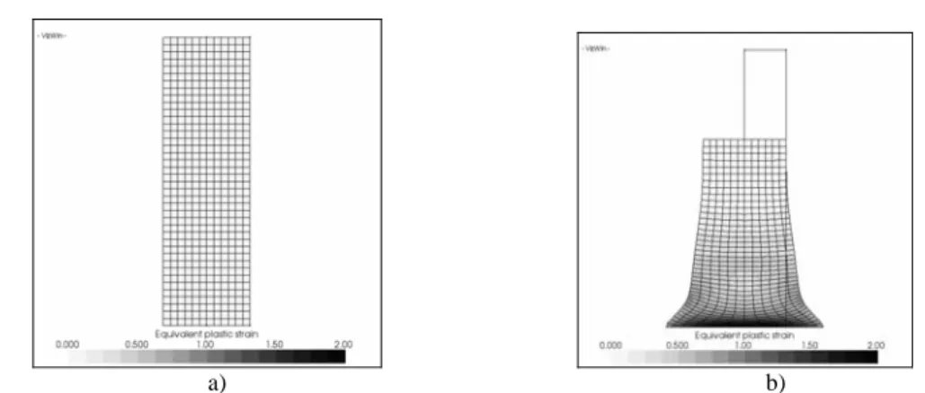
The basic principle is to enhance the strain gradient F of each element an “extended” part such as missing strain modes are added to the 1st degree shape functions. The enhanced strain modes are chosen to circumvent bending and shear locking. To illustrate the locking phenomenon induced by use of classical finite element, a bending dominated problem is considered: a sheet is bended so that an elastic core should appear at the center of the sheet (equivalent plastic strain should be zero) due to pure bending. When using EAS formulation, this elastic core appears with only two elements through the thickness, while ten elements are necessary to obtain this elastic core with classical SRI elements (see Figure 3).
5. APPLICATION: CRUSH ANALYSIS OF THIN-WALLED SQUARE TUBES
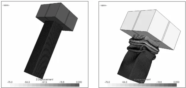
This application takes into account all the developments presented in this paper: thermomechanical formulation, implicit dynamic algorithms, EAS finite elements, constitutive law taking into account strain rate and thermal effects. Simulations of crash of such square tubes provide the deformed shape and the reaction force in order to predict and evaluate the crash-worthiness of a vehicle. The material and geometrical data are presented in [10-11]. The problem consists of the crushing of a thin-walled structure (see
Figure 4
) by a 200kg rigid mass having an initial velocity of 48km/h. The numerical results are presented inFigure 4
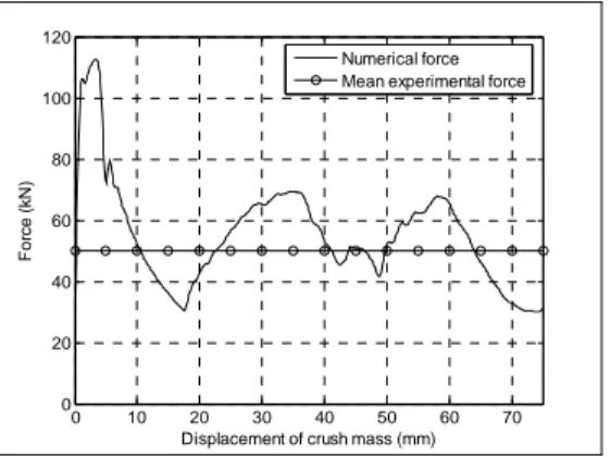
b). The buckling modes appear at the top of structure, what is experimentally observed. The rigid mass displacement-reaction force curve (see Figure 5) corresponds to the experimental observations (see [10-11]).
a) b)
Figure 4. Crushing of a thin-walled square structure: Initial (a) and final (b) configurations
6. CONCLUSIONS
In this paper some essential elements to accurately solve a dynamic problem were presented. Moreover, the CPU and memory cost of the simulation are taken into account in order to solve as efficiently as possible the problem. For that sake, implicit thermomechanical algorithms have been
presented, constitutive laws have been implemented and EAS finite elements were used to avoid a too fine mesh. As presented in the numerical simulations, all this results in an efficient and accurate way to conduct numerical simulations for the large strain, high strain rate thermomechanically coupled problem 0 10 20 30 40 50 60 70 0 20 40 60 80 100 120
Displacement of crush mass (mm)
Fo rc e ( k N ) Numerical force Mean experimental force
Figure 5. Evolution of crushing force
ACKNOWLEDGMENT
This research was carried out under the auspices of the Walloon Region under grant First Objectif 3- IMPAMETA, N° 215275 which is gratefully acknowledged.
References
[1] Johnson G.R. and Cook W.H., “A constitutive model and data for metals subjected to large strains, high strain rates and high temperature”, 7th Int. Symposium on ballistics, The Hague, The Netherlands, (1983) pp. 541-547
[2] Zerilli F.J. and Armstrong R.W., “Dislocation-mechanics-based constitutive relations for material dynamics calculation”, J. Appl. Phys., 5 (1990) pp. 1816–1825
[3] Armero F. and Simo J.C., “A priori stability estimates and unconditionally stable product formula algorithms for nonlinear coupled thermoplasticity”, Int. J. Plast., 9 (1993) pp. 742-783
[4] Adam L., Ponthot J.P., “Thermomechanical modeling of metals at finite strains: First and mixed order finite elements”, Int. J. of Sol. and Str., 42 (2005), pp. 5615-5655
[5] Newmark N., “A method of computation for structural dynamics”, J. Eng. Mech. Div., 85 (1999) pp. 67-94
[6] Géradin M. and Rixen D., “Mechanical vibrations (theory and applications to structural dynamics)”, (John Wiley and Sons, Paris, 1994)
[7] Chung J. and Hulbert G., “A time integration algorithm for structural dynamics with improved numerical dissipations: the generalized-alpha method”, J. Appl. Mech., 60 (1993) pp. 371-375
[8] Andelfinger U. and Ramm E., “EAS-elements for two-dimensional and three-dimensional plate and shell structures and their equivalence to hr-elements”, Int. J. Num. Meth. Eng., 36 (1993) pp. 1311-1337
[9] Bui Q.V., Papeleux L. and Ponthot J.P., “Numerical simulation of springback using enhanced assumed strain elements”, J. Mat. Proc. Tech., 153-154 (2004), pp. 314-318
[10] Huh H., Kang W.J., “Crash-worthiness assessment of thin-walled structures with the high-strength steel sheet”, Int. J. Veh. Des., 30 (2002) pp. 1-21
[11] Noels L., Stainier L. and Ponthot J.P., “Simulation of crashworthiness problems with improved contact algorithms for implicit time integration