Inductive representation, proofs and refinement of pointer structures

THÈSE

THÈSE

En vue de l’obtention du

DOCTORAT DE L’UNIVERSITÉ DE TOULOUSE

Présentée et soutenue le 20 juin 2013 par : Mathieu Giorgino

Inductive Representation, Proofs and Refinement of Pointer Structures

(Représentation Inductive, Preuves et Raffinement de Structures de Pointeurs)

JURY

Rachid Echahed Chargé de Recherche CNRS LIG, Grenoble Louis Féraud Professeur des Universités IRIT, Toulouse Ralph Matthes Chargé de Recherche CNRS IRIT, Toulouse Pierre-Etienne Moreau Professeur des Universités INRIA, Nancy Marc Pantel Maître de Conférence IRIT-ENSEEIHT, Toulouse Martin Strecker Maître de Conférence IRIT, Toulouse Arnaud J. Venet Chargé de Recherche NASA Ames, Mountain View

École doctorale et spécialité :

MITT : Domaine STIC : Sureté de logiciel et calcul de haute performance

Unité de Recherche :

IRIT

Directeurs de Thèse :

Ralph Matthes et Martin Strecker

Rapporteurs :

Je tiens tout d’abord à remercier tous les membres de mon jury au sens large (invités ou non), à commencer par mes rapporteurs Rachid Echahed et Pierre-Etienne Moreau qui ont accepté de prendre le temps de lire et évaluer ce que j’avais pu écrire. Je remercie aussi Marc Pantel pour les cours qu’il a pu me donner et sans qui cette thèse n’aurait pas pu commencer. Merci également à Louis Féraud d’avoir accepté de faire partie de ce jury et à Arnaud Venet pour sa cordialité et son humanité.

Évidement cette thèse n’aurait jamais pu être accomplie sans mes deux directeurs Ralph Matthes et Martin Strecker. Je remercie Ralph pour tous les bons conseils qu’il m’a donné, tirés de son expérience raisonnée et de sa rigueur. J’ai beaucoup apprécié son impartialité teinté d’humanité appliquée aussi bien dans ses travaux scientifiques que dans ses tâches administratives. Un très grand merci à Martin qui m’a suivi tout au long de ses dernières années – en stage puis en thèse – et qui m’a même pratiquement pris par la main pour me montrer ce fabuleux métier qu’est la recherche (et cela même malgré les contraintes qu’il comporte). Merci à lui pour son grand coeur, son enclin à partager ses connaissances scientifiques et sa tendance naturelle à vouloir aider. Je m’excuse auprès d’eux d’avoir été si long à finir.

Je tiens aussi à remercier l’équipe Isabelle de l’université technique de Munich, et en particulier Tobias Nipkow pour m’avoir accueilli pendant 2 mois. Ce fut une expérience réellement enrichissante aussi bien culturellement que scientifiquement. Merci plus par-ticulièrement à Florian Haftman qui a pris de son temps pour me guider dans la TUM, m’installer dans son bureau, s’intéresser à mon travail et me montrer les coulisses d’Isabelle. Merci aussi à Lukas Bulwahn et Jasmin Blanchette.

Toutes ces années à l’IRIT auraient vraiment été ennuyeuses et fades sans mes deux collègues de bureau Celia et Christelle. Merci à Christelle pour nous avoir accueilli dans son bureau, ainsi que pour avoir partagé un peu de sa vie familiale et de ses expériences. Merci à Celia pour tous ses conseils, qu’ils aient été administratifs ou techniques, sa grande gentillesse et ses histoires toujours intéressantes, quoi qu’elle en dise ou quoi que j’ai eu l’air d’en penser ;-). Merci aussi à Mathias pour les discussions scientifiques que nous avons eu depuis son arrivé dans le bureau.

Merci à tous les membres de l’équipe ACADIE qui m’ont accueilli et supporté pendant ces années, c’est à dire son chef bienveillant (et parfois pressant) Mamoun Filali, les permanents et mes collègues doctorants. Merci en particulier à Bertrand pour ses visites de bureau et ses discussions scientifiques à tendences philosophiques et parfois déprimantes ;-). Merci aussi à Selma pour sa gentillesse et sa bonne humeur. Je m’excuse auprès d’elle et de Nadehza pour avoir peut-être monopolisé Martin trop longtemps.

Merci aux collègues de l’IRIT avec qui j’ai partagé de nombreux moments et d’intéressantes discussions, que ce soit pendant les repas au RU, les pauses à la cafét’, la fête de l’IRIT ou les sorties en dehors de l’université. Je cite par ordre de rencontre Anthony, Mathieu, les deux Sylvain, les deux François, Olivier, Guillaume, Victor, Dana, Samir, Philippe, Andra, Magdalina, Vali, Marie, Laure, Rodolphe, Dorian et Florian.

L’administration, bien que déjà complexe serait certainement pire si il n’y avait pas une bonne équipe administrative. Merci en particulier à Arnaude Cariou, Sabyne Lartigue et au service mission. Merci aussi au service technique, et notamment Brigitte Marchiset et Jean-Pierre Baritaud. Merci encore à Martine Labruyère pour sa gentillesse et sa compréhension.

Viennent ensuite tous ceux qui me sont proches et chers: ma famille et mes amis. Que dire tout d’abord à mes parents Christian et Annie, à qui je dois tout, sinon un immense merci. Merci pour l’éducation qu’ils m’ont donné, merci pour leur présence, merci pour leur soutien (qu’il soit matériel ou pas), merci encore. Merci ensuite à ma soeur Magali pour sa gentillesse et ses bons petits plats et à Nicolas qui la rend heureuse. Pour continuer, merci aussi à toute ma famille et en particulier à mes grands parents Yvette, Jean et Angel (je pense aussi à Madeleine), et à mes oncles, tantes et cousins.

Enfin je remercie mes amis. Merci tout d’abord à Delphin qui m’accompagne dans toutes aventures, ski (encore ?), badminton (à reprendre ?), déménagements, technologies, voyages et jeux de sociétés... Merci aussi à Viorica pour les cinés et les soirées mémorables passées ensembles avec Delphin. Merci à Ana-Maria et Ovidiu pour leurs ballades toujours excellentes et bien organisées. Merci à Benoît (Papi) pour l’organisation des quelques voyages dont nous avons profité avec Delphin. Merci de même à Grégory pour les soirées tardives “Little Big Planet” ;-). Un grand merci aussi à Fara pour les bons moments passés ensembles.

Merci également à Martin, à Benoît, à PX, à Pierre et à Eva.

J’ai aussi une pensée pour ceux qui sont loin et que je ne contacte pas assez souvent. Notamment Franck et Elise (je vais venir, promis !), Simon et Isabelle, Jean-Christophe, Valentin et Mohammed.

Pour finir, un immense merci à Monia pour cette merveilleuse année passée.

Remerciements . . . i

Contents . . . iii

List of Figures . . . vii

List of Definitions and Theorems . . . viii

Introduction xi The Contributions in Short . . . xiv

Thesis Layout . . . xiv

I Foundations 1 1 An Example: Cyclic Lists 3 1.1 Cyclic Lists: Informally . . . 3

1.2 Specification with an Inductive Datatype . . . 4

1.2.1 Basics on Inductive Lists and Pairs . . . 4

1.2.2 Definitions of the Cyclic List Specifications . . . 5

1.2.3 Properties of the Cyclic List Specifications . . . 7

1.2.4 Accomplishments . . . 9

1.3 Example Refinement . . . 10

1.3.1 Datatypes . . . 10

1.3.2 Guidelines . . . 11

1.3.3 Function Refinements . . . 12

1.3.4 Inheritance of the Specification Properties . . . 18

2 Scientific Context 21 2.1 Isabelle/HOL . . . 21

2.1.1 Logic and Notations . . . 22

2.1.2 Standard Packages . . . 25

2.1.3 Imperative_HOL . . . 34

2.2 Graph Transformations and Representations . . . 41

2.2.1 A Mathematical View (Raw Pointers) . . . 42

2.2.2 Graph Rewriting Systems . . . 43

2.2.3 Inductive Extensible Adjacency List . . . 48

2.2.4 Trees and Paths . . . 49

2.2.5 Infinite Trees through Coinduction . . . 50

2.2.6 In Short . . . 52 2.3 Program Correctness . . . 52 2.3.1 Hoare Logic . . . 53 2.3.2 Separation Logic . . . 55 2.3.3 Program Verification . . . 56 2.3.4 Refinement . . . 59

2.3.5 Safe Code Generation . . . 60

II Contributions 63

3 Memory Model 65

3.1 Why Imperative_HOL ? . . . 66

3.2 Rough Edges of Imperative_HOL . . . 67

3.2.1 Instantiation of Class countable . . . 67

3.2.2 Local Reasoning . . . 67

3.2.3 Reference Update . . . 69

3.2.4 Some Other Missing Features . . . 69

3.3 Representation of Datatypes in the Heap . . . 69

3.3.1 Examples of (non-)Countable Datatypes . . . 70

3.3.2 Proof that Datatypes are countable . . . 71

3.3.3 Related Work . . . 73

3.4 Proof tools . . . 74

3.5 Objects in Imperative_HOL (Removal of the Ref Class) . . . 75

3.5.1 Example: References in Imperative_HOL . . . 76

3.5.2 Consequences on Code Generation . . . 77

3.5.3 Defining Accessors and Field Update to Remove Indirections . . . . 80

3.6 Objects in Isabelle/HOL . . . 85

3.6.1 Inheritance and Subtyping in Isabelle/HOL . . . 85

3.6.2 Traits in Isabelle/HOL . . . 86

4 Inductive Representations of Pointer Structures 87 4.1 Introduction . . . 88

4.2 A First Example on Singly-Linked Lists . . . 89

4.2.1 Datatypes . . . 89

4.2.2 Refinement Relation . . . 90

4.2.3 Functions . . . 91

4.2.4 Simulation Proof . . . 92

4.2.5 Entailment of Further Properties . . . 94

4.2.6 Conclusion . . . 96

4.3 Formal Refinement of Cyclic Lists . . . 96

4.3.1 Datatypes . . . 96 4.3.2 Functions . . . 97 4.3.3 Conclusion . . . 105 4.4 Possibly-Cyclic Lists . . . 105 4.4.1 Definitions . . . 106 4.4.2 Termination . . . 107 4.4.3 Correctness . . . 108 4.4.4 Refinement . . . 109 4.4.5 Conclusion . . . 110 4.5 Methodology . . . 111

4.5.1 A Classification of Algorithms w. r. t. Graphs . . . 111

4.5.2 The Inductive Structure . . . 115

4.5.3 The Missing Edges . . . 118

III Case-studies 121

5 The Schorr-Waite Algorithm 123

5.1 Introduction . . . 123

5.2 Related Work . . . 125

5.3 Schorr-Waite on Pure Trees . . . 126

5.3.1 Data Structures . . . 126

5.3.2 Algorithms . . . 127

5.3.3 Proofs . . . 129

5.4 Implementation for Pure Trees . . . 131

5.4.1 Data Structures . . . 131

5.4.2 An Imperative Algorithm . . . 132

5.4.3 Correctness . . . 133

5.5 Schorr-Waite on Trees with Pointers . . . 136

5.5.1 Introducing Abstract Graphs . . . 136

5.5.2 Formalization . . . 139

5.6 Implementation for Trees with Pointers . . . 141

5.7 Graphs . . . 142 5.7.1 Definitions . . . 142 5.7.2 Proofs . . . 143 5.8 Conclusions . . . 144 6 BDD Construction 145 6.1 Introduction . . . 145 6.2 Related Work . . . 147

6.3 Binary Decision Diagrams . . . 147

6.3.1 Tree Structure and Interpretation . . . 147

6.3.2 Sharing . . . 149

6.3.3 Ordering and Reducedness . . . 149

6.4 Constructing BDDs . . . 151

6.5 Optimizations: Memoization and Garbage Collection . . . 153

6.6 Implementation of Abstract Functions . . . 154

6.7 Performance Evaluation . . . 155

6.8 Conclusions . . . 157

IV Conclusions and Perspectives 159 Conclusions . . . 161

Perspectives . . . 162

Version française de la thèse 167 Introduction 169 Aperçu des contributions . . . 171

I_fr Fondations 173

1_fr Un exemple : les listes cycliques . . . 173

2fr Contexte scientifique . . . 173 2_fr.1 Isabelle/HOL . . . 173 2_fr.2 Transformations de graphes . . . 174 2fr.3 Validation de programmes . . . 175 II_fr Contributions 177 3fr Le modèle de mémoire . . . 177

4_fr Représentations inductives de structures de pointeurs . . . 177

IIIfr Études de cas 181 5_fr L’algorithme de Schorr-Waite . . . 181 6_fr Construction de BDDs . . . 182 IV_fr Conclusions et perspectives 183 Bibliography 189 Résumé en Français 201 Abstract 202

1.1 Insertion of elements in a cyclic list . . . 4

1.2 Changing the current node in a cyclic list . . . 4

1.3 Simulation for the refinement of ccur to sccur. . . 12

1.4 Simulation for the refinement of ccur1 to sccur1 . . . 13

1.5 Simulation for the refinement of cnext toscnext . . . 14

1.6 Simulation betweenscsingle1 and λx. [x] (or λx. cins x cempty) . . . . 16

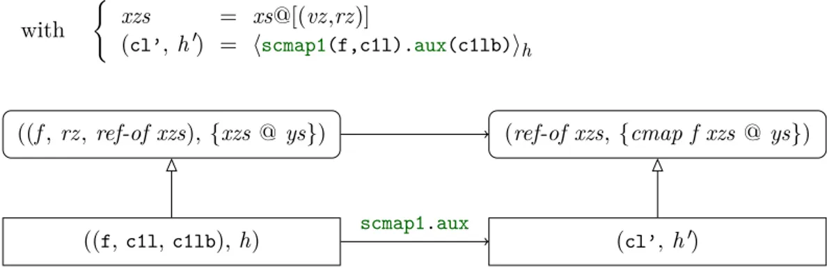
1.7 Simulation for the auxiliary refinement of cmap toscmap1.aux . . . 17

1.8 Simulation for the refinement of cmap toscmap . . . 18

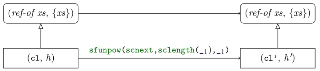
1.9 Simulation for the auxiliary refinement of clength to sclength1.aux . . . 19

1.10 Obtention of a low-level property from the high-level Lemma 1.12 . . . 19

2.1 The Polymorphic Heap of Imperative_HOL . . . 35

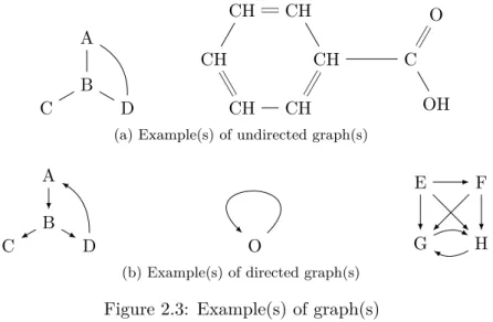
2.2 References in Imperative_HOL, the generated Scala code and the expected one 41 2.3 Example(s) of graph(s) . . . 41

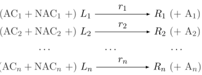
2.4 General Representation of a (graph) rewriting system . . . 43

2.5 The Diagrams of the principal categorical approaches . . . 45

2.6 Structural Rules of the first-order Hoare logic . . . 54

2.7 Axiomatic Semantics of a small imperative language within the Hoare logic 54 2.8 The Frame rule . . . 55

2.9 Axiomatic Semantics of heap related constructs . . . 55

3.1 Types of the example presented in Section 3.5.1 – UML class diagram . . . 76

3.2 Definitions of the FooBar, Foo and Bar classes in Isabelle/HOL, Scala and C++ 78 3.3 Definition of the foofun function in Isabelle/HOL, Scala and C++ . . . 78

3.4 Memory evolution in foofun . . . 79

3.5 Definition of the barfun function in Isabelle/HOL, Scala and C++ . . . 79

3.6 The Reference Primitives of Imperative_HOL, Scala and C++ (brief) . . . 79

4.1 Example of a concrete linked list . . . 90

4.2 Example of a concrete cyclic list . . . 98

4.3 Examples of the execution of the cycle detection algorithm . . . 106

4.4 A Classification of modules: Euler diagram of several module categories. . . 115

5.1 Operations of the Schorr-Waite algorithm. . . 127

5.2 Typical Execution of the Schorr-Waite algorithm . . . 129

5.3 A Tree with additional pointers and the corresponding graph . . . 137

5.4 Two Spanning Trees with additional pointers representing the same graph . 137 5.5 Executions of the low and high-level algorithms with a “good” spanning tree 138 5.6 Executions of the low and high-level algorithms with a “bad” spanning tree 139 6.1 Hierarchies of data and methods . . . 146

6.2 Sharing nodes in a tree . . . 149

6.3 Evaluation of the generated code efficiency . . . 156

Definitions

1.1 Type Definition (list) . . . . . 4

1.2 Definition (append) . . . . 5

1.3 Definition (map) . . . . 5

1.4 Type Definition (clist) . . . . 5

1.5 Definition (cempty) . . . . 6 1.6 Definition (cins) . . . 6 1.7 Definition (ccur ) . . . . 6 1.8 Definition (cnext) . . . . 6 1.9 Definition (cdel) . . . 6 1.10 Definition (clength) . . . . 7 1.11 Definition (cmap) . . . . 7 1.12 Definition (funpow) . . . . 8 1.13 Definition (ccur1 ) . . . 13 1.14 Definition (csingle) . . . . 15

2.1 Definition (Linear notation for term-graphs) . . . . 44

3.1 Type Definition (pheap) . . . 74

3.2 Definition (refs-of ) . . . . 74

3.3 Definition (in-heap-set) . . . 74

3.4 Definition (in-heap) . . . . 74

3.5 Type Definition (raw-ref ) . . 75

3.6 Definition (heap-locally) . . . 75

3.7 Definition (refs-perm) . . . . 75

3.8 Type Definition (accessor ) . . . 81

3.9 Definition (RAcc.acc) . . . 81 3.10 Definition (RAcc.mut) . . . . 82 3.11 Definition (RAcc.upd) . . . . 82 3.12 Definition (RAcc.comp) . . . 82 3.13 Definition (is-acc) . . . 82 3.14 Definition (RAcc.lookup) . . . 83 3.15 Definition (RAcc.update) . . . 83 3.16 Definition (RAcc.mutate) . . 83 3.17 Definition (Ref-map) . . . . . 83 3.18 Definition (RAcc.get) . . . . . 84 3.19 Definition (RAcc.map) . . . . 84 3.20 Definition (RAcc.set) . . . . . 84

3.21 Type Definition (rnode) . . . 84

3.22 Type Definition (any) . . . . 84

3.23 Definition (RNode) . . . . 84

4.1 Type Definition (rlist) . . . . 90

4.2 Definition (rlist-of0) . . . 91 4.3 Definition (rlnodes0) . . . 91 4.4 Definition (lrev-aux) . . . 91 4.5 Definition (lrev) . . . 91 4.6 Definition (rlrev-aux) . . . . . 92 4.7 Definition (rlrev) . . . . 92

4.8 Type Definition (rclist1 ) . . . 96

4.9 Type Definition (rcnode) . . . 96

4.10 Definition (RCNode) . . . . . 96

4.11 Type Definition (rclist) . . . 97

4.12 Type Definition (clist) . . . . 97

4.13 Definition (rclist1-of ) . . . . 97 4.14 Definition (rclist1-ofd) . . . . 97 4.15 Definition (rclist-of ) . . . . . 97 4.16 Definition (rcnodes) . . . 97 4.17 Definition (rcnodes0) . . . 99 4.18 Definition (rccur1 ) . . . . 99 4.19 Definition (rccur ) . . . . 99 4.20 Definition (rcnext1 ) . . . 100 4.21 Definition (rcnext) . . . . 100 4.22 Definition (UndefRef ) . . . 101 4.23 Definition (new-RCList1 ) . . . 101 4.24 Definition (rcsingle1 ) . . . 101 4.25 Definition (rcsingle) . . . 101 4.26 Definition (rcmap1-aux) . . . 102 4.27 Definition (rcmap1 ) . . . 102 4.28 Definition (rcmap) . . . . 102 4.29 Definition (rfunpow) . . . . . 103 4.30 Definition (rclength1-aux) . . 104 4.31 Definition (rclength1 ) . . . . 104 4.32 Definition (rclength) . . . . . 104

4.33 Type Definition (pclist) . . . 105

4.34 Definition (pcnil) . . . . 106

4.35 Definition (pcref ) . . . . 106

4.36 Definition (pcnext) . . . . 106

4.37 Definition (pcyclic-aux) . . . 106

4.38 Definition (pcyclic) . . . . 106

4.39 Type Definition (rpcnode) . . 109

4.40 Type Definition (rpclist) . . . 109

4.41 Type Definition (pclist) . . . 109

4.43 Definition (rpclist) . . . . 109 4.44 Definition (rlnext) . . . 109 4.45 Definition (rlcyclic-aux) . . . 109 4.46 Definition (rlcyclic) . . . . 110 4.47 Definition (Path) . . . 112 4.48 Definition (Successors) . . . . 112 4.49 Definition (Prefix) . . . 112 4.50 Definition (Sharing) . . . 112 4.51 Definition (Cyclicity) . . . 113

4.52 Definition (Algorithm Paths) 113 4.53 Definition (Algorithm Traversal)113 4.54 Definition (Module) . . . 113

4.55 Definition (Shared Paths) . . 113

4.56 Definition (Shape Preservation) 114 4.57 Definition (Cyclic Paths) . . . 114

4.58 Definition (Shared Shape Preservation) . . . 114

4.59 Definition (Static Edge) . . . 118

4.60 Definition (Dynamic Edge) . 118 5.1 Type Definition (tree) . . . . 126

5.2 Type Definition (dir ) . . . . . 126

5.3 Type Definition (tag) . . . . . 126

5.4 Definition (unmarked) . . . . 127 5.5 Definition (sw-term) . . . . . 128 5.6 Definition (sw-body) . . . 128 5.7 Definition (sw-tr ) . . . . 128 5.8 Definition (count) . . . . 128 5.9 Definition (unmarked-count) . 129 5.10 Definition (left-count) . . . . 129 5.11 Definition (mark-all) . . . . . 129 5.12 Definition (t-marked) . . . . . 130 5.13 Definition (p-marked) . . . . 130 5.14 Definition (reconstruct) . . . 130

5.15 Type Definition (stree, srnode) 131 5.16 Type Definition (snode) . . . . 131

5.17 Definition (unmarked-impl) . 132 5.18 Definition (sw-impl-term) . . 132

5.19 Definition (sw-impl-body) . . 132

5.20 Definition (sw-impl-tr ) . . . . 133

5.21 Type Definition (atag) . . . . 133

5.22 Definition (rm-addr ) . . . . . 133 5.23 Definition (add-addr ) . . . . . 133 5.24 Definition (stree-of-tree) . . . 134 5.25 Definition (srnodes-of-tree) . 134 5.26 Definition (config-in-heap) . . 134 5.27 Definition (reach) . . . . 135 5.28 Definition (simul-rel-tree) . . 136

5.29 Type Definition (sgraph) . . . 136

5.30 Definition (t-marked-ext) . . . 139 5.31 Definition (reach-visited) . . . 140 5.32 Definition (p-marked-ext) . . 140 5.33 Definition (marked-as-in) . . 140 5.34 Definition (sgraph-of-tree) . . . 141 5.35 Definition (trancl) . . . 142 5.36 Definition (sstrees) . . . . 142 5.37 Definition (heap-reach) . . . . 143 5.38 Definition (tree-of-graph) . . . 143

6.1 Type Definition (expr ) . . . . 148

6.2 Definition (interp-expr ) . . . 148

6.3 Type Definition (tree) . . . . 148

6.4 Type Definition (rtree) . . . . 148

6.5 Definition (interp) . . . . 148

6.6 Definition (ref-unique) . . . . 149

6.7 Definition (ordered) . . . 150

6.8 Definition (reduced) . . . 150

6.9 Definition (redundant) . . . . 150

6.10 Definition (robdd, robdd-refs) 150 6.11 Type Definition (leaves) . . . . 151

6.12 Definition (wf-heap) . . . 152

6.13 Definition (app) . . . . 152

6.14 Definition (build) . . . . 153

6.15 Type Definition (bddstate-hash) 154 6.16 Definition (add) . . . . 155 6.17 Definition (add) . . . . 155 6.18 Definition (add) . . . . 155 6.19 Definition (gc) . . . 155 6.20 Definition (gc-cond) . . . 155

Theorems

1.9 Lemma (cnext_cmap_swap) 8 1.10 Lemma (funpow_Suc_right) 9 1.11 Lemma (cnext_pow_aux) . . 9 1.12 Lemma (cnext_pow) . . . 9 1.13 Lemma (ccur_ccur1) . . . 13 2.1 Lemma (even0_cases) . . . . 25 2.2 Theorem (return_bind) . . . 37 2.3 Theorem (bind_return) . . . 37 2.4 Theorem (bind_bind) . . . . 37 2.5 Theorem (raise_bind) . . . . 37 3.1 Theorem (ti_encode_inj) . . . 71 4.1 Lemma . . . 91 4.2 Lemma . . . 91 4.3 Lemma . . . 92 4.4 Theorem . . . 93 4.5 Lemma . . . 94 4.6 Theorem . . . 94 4.7 Lemma . . . 94 4.8 Theorem . . . 95 4.9 Theorem . . . 95 4.10 Lemma . . . 99 4.11 Lemma . . . 100 4.12 Lemma . . . 100 4.13 Lemma . . . 100 4.14 Lemma . . . 101 4.15 Lemma . . . 101 4.16 Lemma . . . 102 4.17 Lemma . . . 103 4.18 Lemma . . . 103 4.19 Lemma . . . 103 4.20 Lemma . . . 104 4.21 Lemma . . . 104 4.22 Lemma . . . 105 4.23 Lemma . . . 107 4.24 Lemma . . . 107 4.25 Lemma . . . 107 4.26 Lemma . . . 108 4.27 Lemma . . . 108 4.28 Lemma . . . 108 4.29 Lemma . . . 110 4.30 Lemma . . . 110 5.1 Lemma . . . 130 5.2 Lemma . . . 130 5.3 Lemma . . . 130 5.4 Lemma . . . 131 5.5 Lemma . . . 131 5.6 Lemma . . . 131 5.7 Theorem . . . 131 5.8 Lemma . . . 134 5.9 Lemma . . . 135 5.10 Lemma . . . 135 5.11 Lemma . . . 135 5.12 Lemma . . . 136 5.13 Lemma . . . 136 5.14 Theorem . . . 136 5.15 Lemma . . . 140 5.16 Lemma . . . 141 5.17 Lemma . . . 141 5.18 Lemma . . . 141 5.19 Theorem . . . 142 5.20 Lemma . . . 143 5.21 Theorem . . . 144 5.22 Theorem . . . 144 6.1 Theorem . . . 150 6.2 Lemma . . . 151 6.3 Theorem . . . 151 6.4 Theorem . . . 153 6.5 Theorem . . . 153 6.6 Theorem . . . 153

How to convince ourselves that a piece of software is failure-free? In a world where our lives increasingly depend on technologies, what are the guarantees that the computations performed by the product of an engineering process really return what we expect from them? These questions certainly are of little interest when applied to your web browser. But what about them when they deal with the software that is composed by – or that has been used to obtain – the bits governing the plane you are in, the car of a friend or the (expensive) rocket that has been launched above our heads?

Until recently, these programs were exclusively validated through tests, executing the programs in a (possibly huge) set of cases to check their outputs were consistent with their

specifications. The problem is that we are unable, in general, to test all the possible behaviors

of a given program, leading invariably to unchecked cases where the program could fail. Tests are the only way to go in the concrete world where exhaustiveness and certainty are pure illusion. It is not in computer science where programs are taken to be mathematical objects.

Indeed, the essence of mathematics is their ability to derive statements from other ones such that no doubt can be phrased on their conformity w. r. t. their assumptions. The same can be done on programs where the correctness of one program can be proved to conform to the correctness of another one, possibly simpler and less efficient. This process called

abstraction can be iterated until obtaining a so-called specification exactly embodying the

idea we could have on the intended behavior of the program. Given the program is always written to satisfy a need translatable into an at least informal specification, this process can also be reversed in a so-called refinement chain ensuring the final program to conform to the initial specification.

Validation of industrial critical systems – that are entities whose failure has to be prevented at all costs – is thus evolving towards more formal and mathematical approaches:

formal methods. However, this can not be done as easily as it could seem, notably because

of the lack of tools, support and knowledge. Moreover, formal methods necessarily add an extra complexity leading to the introduction of constraining industrial standards for the development of programs. These constraints especially have an impact on the efficiency of the program by preventing for example the use of memory allocation or pointers.

Also the question of the faith we can have in the provided proofs is slowing down the efforts that would be necessary to obtain a wide use of formal methods in industry. A part of the available tools are built around a small (and thus manually verifiable) certified kernel through which all the proof steps are checked, but using several of them can rapidly enlarge the trusted code base. A set of them whose objective is to provide a framework in which a huge number of applications can take place – thus reducing by the same number the size of the trusted code base – are called general purpose proof assistants.

In this thesis, we are interested in providing methods – aimed at an industrial context – to carry out refinement proofs involving pointer structures in proof-assistants from which we chose Isabelle [113]. The first word of the thesis title (inductive) – the only one which has not been covered by this introduction – is what gives it its originality. We elaborate on this and all the other concepts in the following.

Initial Motivation

Model-Driven Engineering (MDE). This PhD thesis draws its initial motivation from the Topcased [58] project. This project was interested in providing tools for the development and certification of critical systems using model-driven approaches. Such approaches encourage the specification of the different views of a system as models being (often graphical) representations of specifications. These specifications are defined as graphs with the informal semantics (and the graphical syntax) provided by UML [80, Unified Modeling Language]. To construct, combine or update these specifications, one can define graph (model) transformations to ensure a uniform modification, and provide a concrete object that can be analyzed or formalized. These transformations evidently also have to be as efficient as possible.

Formalization in proof assistants. The formalization and validation of these graph transformations then had to be performed. Previous work had been conducted to verify properties on graph transformations based on automated tools such as model-checker like MONA [82, 109]. It appeared that both the limitation to Graph-Types [81] and the combinatorial explosion was preventing to consider them to verify real-world systems. Instead, we switched to interactive provers (also called proof assistants) to benefit from their generality and their means to guide the proofs.

An Efficient Implementation

Pointer Structures. An efficient representation of graphs has to provide easy and fast accesses to arbitrary nodes, as well as avoiding too much duplication, to prevent unnecessary consumption of the resources giving all the legitimacy to computer science: time and space. Such properties can be satisfied with pointers that provide access to data through their addresses. As a consequence, several pointers to the same data can be used to read or write it from different locations. This can be seen as a space savings – given that the data does not need anymore to be duplicated – or as a time savings – given that the data can be accessed directly (by its address) instead of being found through other paths or that the result of a computation can be put into a shared data to be directly available from other locations. With explicit pointers, the nodes of the graphs can be represented by records in a heap and edges can be represented by pointers between these records. To represent such mechanisms, we use the library Imperative_HOL – provided by Isabelle/HOL – that introduces a shallow embedding of an imperative language allowing to manipulate pointers. By using Imperative_HOL, we discovered some shortcomings that we solved and present.

In an object-oriented (OO) language. Proof assistants in general and Isabelle/HOL in particular provide means to extract executable definitions through code generation into different languages. This mechanism is also available for Imperative_HOL. In order to be widely usable, the generated code has to be in a language close from those commonly used (for example in industry), while being sufficiently close from the language furnished by the proof assistant to allow a straightforward (and easily verifiable) translation. Scala [114, 145] – a modern language unifying the OO and functional paradigms in a seamless way – appeared to be perfectly fitted to this task. Besides the advantage of such a combination, it also compiles to the Java Virtual Machine (JVM) so that Scala and Java are interoperable,

meaning that Scala can benefit from the huge number of libraries available for Java while Java developments can easily use Scala ones.

Scala is supported as a target language of the code generator of Isabelle/HOL, however, it is not always optimized or idiomatic. To improve this code generation, we suggest in this thesis a shallow embedding of OO constructions in Isabelle/HOL and highlight the

Isabelle/HOL counterparts of some OO mechanisms that should allow to obtain code that

would be both valid and easy to use.

A Practical Representation as Inductive Datatypes

Verification of programs manipulating pointers is an active research domain that has proved to be difficult. All the problems inherent to the manipulation of pointer structures are still present in Imperative_HOL that only provides means to define imperative programs in Isabelle/HOL. Instead of fighting against such problems, we propose to start from a practical abstraction of pointer structures that could be refined later to imperative programs.

Inductive datatypes. The proof assistants providing support for program development are in the vast majority based on functional languages whose semantics is sufficiently close to mathematical concepts to be also useful for the development of abstract theories. In such languages, the manipulated data are to a large extent built from (co)inductive datatypes, that are a means to define (possibly infinite) tree datastructures whose shapes are constrained by types. As a consequence, it is hard to find a direct representation of pointer structures as shared or cyclic graphs and to reason about them in a proof-assistant.

For tree-shaped graphs. However, the difficulties stems from the extra assumption that the pointer structures should be represented in all their generality, without discriminating some cases to favour others. We however find ourselves in the case where the graphs that we want to represent arise from models that seem to be commonly tree-shaped, i. e. with a natural spanning tree standing out. Indeed, edges of models are often split into several categories – such as inheritance or composition relations in class diagrams – which ease the identification of their skeletons, thanks to the possibility to give an emphasis on a particular category.

With this general background assumption that a spanning tree can be extracted more or less easily from the manipulated pointer structures, this work describes the methods and

needed restrictions to represent graphs and graph transformations by inductive datatypes (trees) and recursive functions.

Extended to more general graphs. We will also see that this representation can be applied for graphs without obvious spanning tree, as long as some other restrictions on the algorithms hold. Indeed, the idea of representing a graph with a tree evidently does not come out without inconveniences. Trees are strictly less general than graphs but that is also their limitations that are their strength when it comes to verify properties about them.

Refined to pointer structure. A refinement can then ensure that the algorithms at high and low-levels preserve the simulation relation between the inductive representation and the pointer structure. We show that the inductive representation we choose simplifies

the refinement by enabling a direct correspondance between the two and we also provide some tools to ease this refinement.

The Contributions in Short

Here, we summarize the 4 main contributions of this thesis that we have already discussed before:

• The representation of pointer structures by inductive datatypes easily manipulated in proof assistants

• Tools for the refinement of this inductive representation to an efficient imperative code • A shallow embedding of some OO features to improve the code generation into a

propitious language

• Two substantial case-studies demonstrating the practicality of the representation

Thesis Layout

In an introductory example (Chapter 1), we first illustrates the intended workflow we propose to obtain correct programs manipulating pointer structures. It describes an inductive representation of cyclic lists allowing to specify common operations on them, that is followed by an implementation in Scala, informally proved to refine the inductive specification.

Chapter 2 contains an overview of the scientific context in which this work has been realized. It starts with Section 2.1 that gives a glimpse on Isabelle and the tools it provides. These ones, and especially the library Imperative_HOL will be used in the rest of the thesis. This is followed by an examination of the existing works regarding representations and transformations of graphs (Section 2.2) and correctness of programs (Section 2.3).

Our contributions are presented in Part II, organized in two Chapters. The first one (Chapter 3) explains the difficulties we encountered with Imperative_HOL and the solutions we propose to get rid of them. It also describes an extension to manipulate objects in Imperative_HOL that is used in the several examples of the following Chapters and it gives considerations towards a better integration of a shallow embedding of object-oriented developments in Isabelle. The second one (Chapter 4) more thoroughly presents the workflow we propose to represent pointer structures by inductive datatypes. This is done by means of examples followed by a general methodology exhibiting two kinds of representations.

Part III is devoted to two substantial case studies that have been carried out using the tools and principles described in the previous sections. Each of them illustrates one kind of the representations presented in Chapter 4.

The last Part IV presents perspectives and future work based on the conclusions that can be drawn from this thesis.

An Example: Cyclic Lists

This chapter presents the intended workflow we propose in this thesis. This is done through the example of cyclic lists represented as inductive lists and for which functions are defined. The datatype is later implemented in Scala by a concrete datastructure with pointers, and the functions are informally refined to their Scala counterparts.

Contents

1.1 Cyclic Lists: Informally . . . . 3

1.2 Specification with an Inductive Datatype . . . . 4

1.2.1 Basics on Inductive Lists and Pairs . . . 4

1.2.2 Definitions of the Cyclic List Specifications . . . 5

1.2.3 Properties of the Cyclic List Specifications . . . 7

1.2.4 Accomplishments . . . 9

1.3 Example Refinement . . . . 10

1.3.1 Datatypes . . . 10

1.3.2 Guidelines . . . 11

1.3.3 Function Refinements . . . 12

1.3.4 Inheritance of the Specification Properties . . . 18

1.1

Cyclic Lists: Informally

We are interested in representing graphs in a proof assistant with the objective to define and prove transformations on them. We take cyclic lists as an example. They are certainly the simplest non-trivial cyclic data structure dually to linked-lists that are the simplest non-trivial acyclic data structure.

A cyclic list can be seen as a sequence of elements from which one is designated as the current one. It is possible to read (ccur ) and delete (cdel) the current element, as well as to insert an element (cins). It is also possible to obtain a handle to the successor of the current element (cnext). In this case, the previous current element becomes the last element in the new sequence obtained.

The cyclic list is handled through a pointer that we will call p. In opposition to what would be done in an immediate first thought, the current node is not the one directly pointed to by p but the following one. Indeed, this allows the cyclic list to behave in a similar way as usual linked-lists for operations like cins and cdel. This is due to the fact that we have to restore the next pointer of the previous element of the node being deleted or inserted. Then it is more natural to point to the last element and to do modifications on the head rather than to point to the first element and to do modifications on the second one.

⊥ p p _{00 0} 1 p ₀ 2 1 p

cins 0 cins 1 cins 2

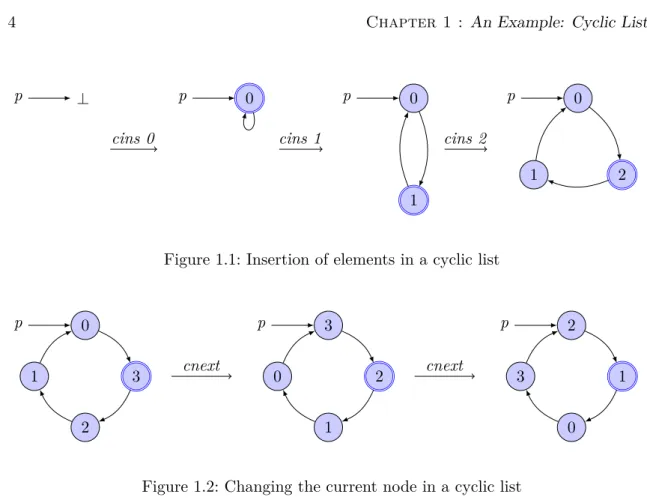
Figure 1.1: Insertion of elements in a cyclic list

0 3 2 1 p ₃ 2 1 0 p ₂ 1 0 3 p cnext cnext

Figure 1.2: Changing the current node in a cyclic list

To have a better intuition, Figures 1.1 and 1.2 graphically show insertion of elements and successive changes of the current node in a cyclic list. The current node is circled twice in blue while the entry point in the cyclic list is pointed by p.

1.2

Specification with an Inductive Datatype

We will now specify cyclic lists with an inductive datatype in Section 1.2.2, prove properties on them in Section 1.2.3 to finally refine them to Scala code in Section 1.3. To be more concrete, we will represent cyclic lists in the functional language provided by Isabelle/HOL. As a support to the following sections, we first describe the predefined 0a list datatype with

its usual operations in Section 1.2.1.

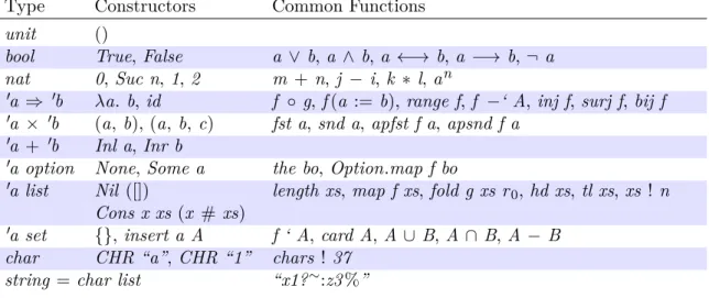
1.2.1 Basics on Inductive Lists and Pairs

Lists Lists are defined classically as an inductive datatype with two constructors Nil (noted []) – representing the empty list – and Cons x xs (noted x # xs) – representing the

insertion of an element x in front of xs:

Type Definition 1.1 (list)

datatype 0a list = Nil | Cons 0a (0a list)

We use a notation for explicit lists that allows to write [0 , 1 , 2 ] for 0 # (1 # (2 # [])). Ubiquitous operations on lists include append xs ys (Definition 1.2, noted xs @ ys, right-associative) – appending the list xs in front of the list ys – and map (Definition 1.3) –

that applies a function on all the elements of a list. append can be shown to verify Lemmas 1.1 and 1.2.

Definition 1.2 (append)

fun append :: 0a list ⇒ 0a list ⇒ 0a list where append [] ys = ys

| append (x#xs) ys = x # (append xs ys)

Definition 1.3 (map)

fun map :: (0a ⇒ 0b) ⇒ 0a list ⇒ 0b list where map f [] = []

| map f (x#xs) = f x # (map f xs)

Lemma 1.1 (append_Nil_right). xs @ [] = xs

Lemma 1.2 (append_assoc). xs @ ys @ zs = (xs @ ys) @ zs

Proof. Trivial with an induction on xs and the definition of append (Definition 1.2).

Pairs In the following, we will also use pairs which are one of the basic datatypes of Isabelle/HOL, used for example to build other tuples and records. Their type is represented as a cartesian product 0a × 0b where 0a and 0b are respectively the types of the first and

second component of the pair. They are represented classically as (a, b) where a is the first component and b is the second, which can respectively be retrieved with the functions fst and snd such that for example fst (a, b) = a. Also the function apsnd (and apfst) allow to update a component of a pair such that for example: apsnd f (a, b) = (a, f b)

1.2.2 Definitions of the Cyclic List Specifications

Following the description of cyclic lists in introduction of Chapter 1, a cyclic list can easily be seen as a list on which operations are applied back to the start of the list when these ones reach its end. We then represent cyclic lists in the functional language provided by Isabelle/HOL. To make clear that we use lists as a representation for cyclic lists, we define a type synonym (0r , 0a) clist simply standing for the type of lists containing pairs of a reference

of type 0r and a value of type 0a associated to it:

Type Definition 1.4 (clist)

type-synonym (0r , 0a) clist = (0r × 0a) list

The fact that we use a pair of a reference and a value will be better justified later (cf. Section 1.3.2). However, we can give the intuition that these references will already give access to the representation of the shape in the heap at the specification level. In this way, properties like aliasing will be easily manipulated at an abstract level to be propagated downwards at the refinement step. As we will see, these references almost won’t impact the algorithms we will define, and will be of great help during the refinement step.

Then the several operations we would like to provide on cyclic lists can be defined. The first ones are the constructors allowing to build an empty cyclic list (cempty) and to insert an element in a cyclic list (cins):

Definition 1.5 (cempty)

definition cempty :: (0r , 0a) clist where cempty ≡ []

Definition 1.6 (cins)

definition cins :: (0r ∗ 0a) ⇒ (0r , 0a) clist ⇒ (0r , 0a) clist where cins x xs ≡ x # xs

Obviously, the constructors of cyclic lists directly correspond to the ones on lists and could then be defined as simple abbreviations of them. In the following, we could always interchange them, and we will consequently prefer the list notation as the more readable one, unless the use of the clist notation emphasizes the refinement relation.

Given that we can now construct cyclic lists, it would be interesting to be able to obtain the value they contain back. The value of the current node of the list will be obtained with the ccur function. However, as a cyclic list can be empty, it is not always possible to satisfy this wish and the function thus uses the type 0a option to represent an optional result

constructed with the help of its two constructors None – for an empty result – and Some x – for a result x.

Definition 1.7 (ccur )

fun ccur :: (0r , 0a) clist ⇒ 0a option where ccur [] = None

| ccur (x#xs) = Some (snd x)

This function is similar to the common head or hd operations that possibly obtain (if the list is not empty) the first value of a list with a simple pattern matching of the list on its constructors. To access the other values, we also need a means to change the current node. To this purpose, we define the cnext function that shifts the list of one node forward.

Definition 1.8 (cnext)

fun cnext :: (0r , 0a) clist ⇒ (0r , 0a) clist where cnext [] = []

| cnext (x#xs) = xs @ [x]

This function is interesting as it is the first one to reveal the potentially cyclic aspect of the representation. Indeed, it puts the first element of the list to its end so that it could be accessed again after the traversal of all the other nodes. To complete the set of primitive functions on cyclic list, we define the function cdel which removes the current node. It returns the updated list and we chose to return an empty list in the case of the empty list to avoid particular cases:

Definition 1.9 (cdel)

fun cdel :: (0r , 0a) clist ⇒ (0r , 0a) clist where cdel [] = []

| cdel (x#xs) = xs

Until then all the defined functions were non-recursive. Let’s see how this representation deals with recursion by defining a clength function returning the length of a cyclic list

(Definition 1.10). It is exactly the definition of the equivalent length on lists and we can effectively trivially prove the equality (Lemma 1.3).

Definition 1.10 (clength)

fun clength :: (0r , 0a) clist ⇒ nat where clength [] = 0

| clength (x#xs) = 1 + clength xs

Lemma 1.3 (clength_is_length). clength xs = length xs

Proof. length and clength have the same definition, i. e. are fixpoints of the same recursive

equations. Also, a proof by induction on xs leads to the result by immediate application of the induction hypothesis.

The same holds for the cmap function as a counterpart of the map function on inductive lists allowing to apply a function on all the elements of a list (Definition 1.11). It is almost the definition of map on lists and we can effectively prove the equality (Lemma 1.4).

Definition 1.11 (cmap)

fun cmap :: (0a ⇒ 0b) ⇒ (0r , 0a) clist ⇒ (0r , 0b) clist where cmap f [] = []

| cmap f (x#xs) = (apsnd f x)#(cmap f xs)

Lemma 1.4 (cmap_is_map). cmap f xs = map (apsnd f ) xs

Proof. By induction on xs, application of the definitions of map and cmap (Definitions 1.3

and 1.11) and the induction hypothesis suffices to conclude.

Contrary to the intuition we would have about cyclic lists, these two functions do not need to look at references to stop. The case where a complete cycle has been done is replaced by the terminal case of cmap with the empty list of the specification. This empty list then embodies at the same time the case where the imperative cyclic list is itself empty and the case where the imperative algorithm has reached again the first node it traversed.

1.2.3 Properties of the Cyclic List Specifications

We can now easily prove properties about these functions standing for the specification of cyclic lists. As soon as the refinement of this specification into an implementation is done, all properties proved on the specification will be available for the implementation. Thus proofs are easily carried out on the abstract level to be usable on the concrete one.

For example, it is easy to show that removing with cdel an element inserted with cins leads to the initial list (Lemma 1.5). We can also prove the usual properties of map for cmap (Lemmas 1.6 to 1.8).

Lemma 1.5 (cdel_cins). cdel (cins x xs) = xs

Lemma 1.6 (cmap_cins). cmap f (cins x xs) = cins (apsnd f x) (cmap f xs) Lemma 1.7 (cmap_append). cmap f (xs @ ys) = cmap f xs @ cmap f ys Lemma 1.8 (cmap_cmap). cmap g (cmap f xs) = cmap (g ◦ f ) xs

Proof. By induction on xs with the definitions of cmap, cins and append (Definitions 1.11,

1.6 and 1.2) together with the one of function composition comp (noted f ◦ g).

As said earlier, the only function defined so far which is really taking into account the cyclic aspect of the list is cnext. The previous lemmas were dealing with classical functions on inductive lists, which is what explains their simplicity. We can now start to prove properties dealing with cnext, as for example the commutativity of cnext and cmap:

Lemma 1.9 (cnext_cmap_swap). cnext (cmap f xs) = cmap f (cnext xs)

Proof. By induction on xs:

• if xs is the empty list, the definitions of cmap and cnext (Definitions 1.11 and 1.8) suffices.

• if xs is x # xs0_{, after application of the definitions of cmap and cnext (Definitions 1.11}

and 1.8) and the inductive hypothesis, we have to prove:

cmap f xs0@ [apsnd f x] = cmap f (xs0 @ [x])

which follows from Lemma 1.7 and the cmap definition (Definition 1.11).

We can see that the proof stays really simple even though the property refers to cnext. Indeed it uses only induction and rewriting of definitions or other simple properties. This is due to the fact that a similar property exists for inductive lists: map f (x # xs) = f x #

map f xs. To show that proofs can stay simple even in cases of properties specific to cyclic

lists, we show that applying cnext as many times as the number of nodes in the list leads to the initial list.

To this purpose we define power of functions as funpow (noted fn for f applied n times). It uses the inductive representation of natural numbers from the Peano axioms [72] usually used in proof assistants. Their constructors are 0 representing zero, and Suc n representing the successor of n (i. e. n + 1 ).

Definition 1.12 (funpow)

fun funpow :: nat ⇒ (0a ⇒ 0a) ⇒ (0a ⇒ 0a) where funpow 0 f = (λx. x)

| funpow (Suc n) f = f o (funpow n f )

In this definition we chose to compose functions on the left. However, as the composed functions within funpow are all the same, we can also show the equation for right composition:

Lemma 1.10 (funpow_Suc_right). fSuc n = fn ◦ f

Proof. By induction on n and application of the definition of funpow (Definition 1.12) and

simplifications of operations on natural numbers.

The proposition to prove then looks like: cnextclength xs xs = xs. However this property

is not directly inductive and needs thus to be generalized first to this auxiliary lemma:

Lemma 1.11 (cnext_pow_aux). cnextclength xs (xs @ ys) = ys @ xs

Proof. By induction on xs and generalization on ys (i. e. application of the induction schema

on the goal universally quantified on ys).

• if xs is [], application of append, funpow and clength definitions (Definitions 1.2, 1.12 and 1.10) with Lemma 1.1 allows to reduce the goal to ys = ys which is true by reflexivity of =.

• if xs is x # xs0_{, application of Lemmas 1.2 and 1.10 with the definitions of cnext,} append and clength (Definitions 1.8, 1.2 and 1.10) and arithmetic simplifications allows

to conclude.

Then the desired goal is a direct consequence of this last lemma:

Lemma 1.12 (cnext_pow). cnextclength xs xs = xs

Proof. Directly results from Lemma 1.11 where ys is instantiated with the empty list [],

followed by the applications of Lemma 1.1 and definition of append (Definition 1.2).

1.2.4 Accomplishments

Inductive lists enabled us to specify all the operations we needed on cyclic lists. When functions on cyclic lists are defined, we can remove the parts of the cyclic list that are not needed for the other calls of the function body (and especially the recursive calls). This means that we can take benefit from the known restrictions of the several calls to simplify the specification. In this case, this allowed to easily prove properties on cmap where the first node of the list was not transmitted to the recursive calls (Lemmas 1.6 to 1.9 and implicitly the termination).

This is the same principle that applies for the returned value, excepted that this value can be used by any other function. In this case, we don’t need to return the cyclic list if it has not been modified, as for example in ccur or clength. On the contrary, the cyclic operation embodied by cnext has been specified to return the entire cyclic list with a call to append, so that the dereferencing of the last pointer is replaced by the computation of

1.3

Example Refinement

This section presents an example implementation of cyclic lists in Scala, with a taste of the refinement proofs that will be more formally developped in Section 4.3.

1.3.1 Datatypes

We first define the typeSCList1[A]of non-empty purely cyclic lists as a class in Listing 1.1. It contains two variable attributes value – for the value of the node – andnext – for the next node in the list.

class SCList1[A](var value:A, var next:SCList1[A])

Listing 1.1: Scala – Definition of the type of non-empty purely cyclic lists

Listing 1.2 defines the typeSCList[A] of cyclic lists. It is composed of the sum of the types of empty cyclic list SCEmpty and of non-empty cyclic listsSCCons[A]. Naturally the

valueSCEmptyrepresents the unique empty cyclic list while the valueSCCons[A](cl) contains an attribute of typeSCList1[A]representing a non-empty cyclic list.

sealed trait SCList[+A]

case object SCEmpty extends SCList[Nothing]

case class SCCons[A](cl:SCList1[A]) extends SCList[A]

Listing 1.2: Scala – Definition of the type of possibly empty purely cyclic lists It follows an algebraic (inductive) definition of types – i. e. a sum of type products (called variants) – where the recursion can only occur on the global (sum) type. In Scala, this is done through the use of case classes (for the variants) – for automatic definition of pattern-matching, constructors, ... – and subtyping (for the type sum). This contrasts with the equivalent definition in Listing 1.3 (where "equivalent" means that the two versions of

SCList[A]describe sets of equivalent values, with potentially distinct use cases) that uses a recursive call to the variantSCList1[A].

sealed trait SCList[+A]

case object SCEmpty extends SCList[Nothing]

case class SCList1[A](var value:A, var next:SCList1[A]) extends SCList[A]

Listing 1.3: Scala – Definition of the type of cyclic or acyclic lists with a recursion on the variantSCList1[A]itself

Thus Listing 1.3 would not be definable in this way using only algebraic datatypes such as those provided by usual functional languages. Indeed, the variants of an algebraic datatype don’t have a specific individual type that would allow to call them recursively. This is possible in Scala thanks to the homogeneous use of classes for the variantsSCEmpty

and SCList1[A]and the sum typeSCList[A].

Another very close version is presented in Listing 1.4 such that the recursion does not occur anymore on SCList1[A]itself. In this case, we replaced SCList1[A] bySCList[A]and

thus added acyclic lists in the values contained inSCList[A]. It then introduces the need to check whether the next element is empty at each step of a traversal of a list, even though this list is cyclic and that once it contains at least one element, all of them have a non-empty successor.

sealed trait SCList[+A]

case object SCEmpty extends SCList[Nothing]

case class SCList1[A](var value:A, var next:SCList[A]) extends SCList[A]

Listing 1.4: Scala – Definition of the type of cyclic or acyclic lists

We also note that Listings 1.3 and 1.4 usecase classes with variable attributes which is not a recommanded practice for the automatic definition of the methodhashCode (provided

by caseclasses) that should be time-invariant, with respect to its specification in the class

Anyeven if we don’t use it in this case. Moreover, variable attributes can generally introduce cyclicity – and this is further enforced by the type of Listing 1.3 – which prevents the termination of the automatically generated methods. Although this does not cause any trouble if the problematic methods are overloaded, or if we replacecase classes by classes with extractors we choose to work with Listing 1.2 which will give less verbose algorithms than Listing 1.4 and a little more verbose than Listing 1.3 but that will be more easily formalized in the functional language of Isabelle/HOL and its common algebraic datatypes (cf. formalization in Section 4.3).

1.3.2 Guidelines

In the following we will define the functions corresponding to the specification of Section 1.2.2 in Scala. Each of these functions will be split into two definitions working on the two types

SCList1andSCList. Naturally, the functions working on possibly empty cyclic lists (SCList)

will use the functions on non-empty cyclic lists (SCList1).

The use of Scala for this example is motivated by our aim to generate code from verified algorithms into Scala that is highly compatible with Java, largely used by industry. However to prove that they are refinements of the previous specifications we would need a formalization of this langage in the verification tool (in our case Isabelle/HOL), which is currently not available and out of reach because of its great complexity. In a first place, we will only visualize the refinements through diagrams and the proofs will only be outlined. A more formal description supported by Isabelle/HOL is given in Section 4.3.

An example diagram is Figure 1.3 (page 12). The top nodes contain the abstract values while the bottom nodes contain the concrete ones. The abstract values are pairs of a value and a set of lists representing the cyclic lists allocated in the heap. The concrete values are pairs of a corresponding value and a heap, that can be the result of the evaluation of an imperative statement on a heap (which returns a value and a possibly modified heap). Concrete and abstract values are related by a refinement property that is used as a hypothesis on the left and as a conclusion on the right. Each refinement property depends on the type of the related values. For example, the refinement on the typeSCList1[A] of non-empty cyclic lists will assume that the representing list is non-empty while the relation on the type

SCList[A]won’t.

Incidentally, the refinement property relating a cyclic list to its specification as an inductive list is the central point of the approach. We recall that the data structure will finally be allocated in a heap by nodes (SCList1) at some addresses and linked by pointers

(through their next attributes). To ease the proof of refinement, we have already attached to each value of the list the reference of the corresponding node in the heap, with the help of a pair whose second component will be the value. In this way, references and values are closely related and the shape of the list in the heap will be easily defined.

This relation has to describe the values in the nodes allocated in the heap and constituting the cyclic list, i. e. the content of this list (thevalue field) together with its shape (the next

field). The pairs of references and values in the specification list already directly describe the content of the cyclic list. Its shape is mostly described by the references in the list combined with the inductive aspect of the list, which gives a successor relation between references. However, this successor relation is acyclic and thus incomplete for a cyclic list which also needs an additional pointer from the last node to the first one. This missing link is then provided by an additional predicate in the refinement relation.

To sum up, the specification list provides all the information needed to construct the cyclic list, either in a straightforward way for the values and the major part of the shape of the cyclic list, or through an additional predicate for the missing part of the shape.

1.3.3 Function Refinements

Evaluation of an imperative statement (for examplesccur(cl)) on a heap h is represented as h_i_h (hsccur(cl)ih) which stands for the pair of the value this statement returns and

the new heap obtained after its execution on h. For example, in this case, the simulation relation states that under the hypothesis that a cyclic list is handled through a node c1lin a heap h and that its representation is a non-empty list xs, the execution of sccur(cl) on

the heap h returns the value ccur xs without modifying h (i. e. h0= h).

The function ref-of allows to retrieve the reference of the pointed element of a cyclic list,

i. e. the reference of the last element of the specification list.

1.3.3.1 Retrieving the current element of a cyclic list

The functionsccur defined in Listing 1.5 refines ccur (Definition 1.7):

def sccur1[A](c1l:SCList1[A]):A = c1l.next.value

def sccur[A](cl:SCList[A]):Option[A] = cl match {

case SCEmpty => None

case SCCons(c1l) => Some(sccur1(c1l)) }

Listing 1.5: Scala – Definition ofsccur1andsccur: retrieves the current value of a cyclic list

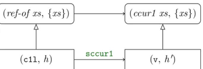
The simulation relation to prove is pictured in Figure 1.3. with (v, h0) = hsccur(cl)i_h

(ref-of xs, {xs}) (ccur xs, {xs})

(cl, h) sccur (v, h0)

Figure 1.3: Simulation for the refinement of ccur to sccur

As the function sccur uses the function sccur1, we could either unfold the definition

allows to factorize proofs. This intermediate step towards the verification of the refinement of ccur for possibly empty cyclic list can be either seen as being part of the proof – if we think it is not relevant for the users of the cyclic lists – or as being an extension of the specification taking into account non-empty cyclic lists. In the second case, the need for this addition comes from the fact that the specification did not take into account this particular refinement and thus the intermediate steps that could be necessary to carry out the proof. Then the specification need be adapted (as it will have to be generalized in the proof of the recursive functions): in the same way as any pragmatic development, we can switch up and down between the specification and the implementation. We consequently build an abstraction ccur1 ofsccur1 that will also use the datatype from the specification of possibly empty cyclic lists.

Definition 1.13 (ccur1 )

fun ccur1 :: (0r , 0a) clist ⇒ 0a where ccur1 (x#xs) = snd x

| ccur1 [] = undefined

We let this function undefined for the empty list as this case will never occur in the refinement. Moreover we can also express ccur with it:

Lemma 1.13 (ccur_ccur1). xs 6= [] =⇒ ccur xs = Some (ccur1 xs)

We can now prove the refinement relation presented in Figure 1.4. with (v, h0) = hsccur1(c1l)i_h

(ref-of xs, {xs}) (ccur1 xs, {xs})

(c1l, h) sccur1 (v, h0)

Figure 1.4: Simulation for the refinement of ccur1 tosccur1

Proof outline for Figure 1.4. There are two properties to verify:

• for the value: asc1lis represented by xs,c1lis the last reference in xs. Thenc1l.next

is the first reference in xs andc1l.next.valueis the corresponding value, that is ccur1

xs.

• for the heap: it stays unchanged as there is no operation (including sccur1) that modifies it in the function.

Here we can see the proof relies on the order of the values provided by the list, which simplifies the management of references.

Finaly this result allows to easily prove the refinement relation of Figure 1.3 for ccur.

Proof outline for Figure 1.3. This relation can be proved by analysing the different possible

cases occuring in the specification ccur xs, i. e. a case distinction on xs. In the both cases, it is simple to verify that the specification and the implementation return the same value as soon as clis represented by xs:

• if xs is empty thencl=SCEmpty and the result isNone

• if xs is not empty thencl=SCCons(c1l)andc1lis also represented by xs, thus the result isSome(sccur1(c1l))with hsccur1(c1l)i_h simulated by ccur1 xs from Figure 1.4,

i. e. the result is simulated by ccur xs from Lemma 1.13.

Also the heap stays unchanged as there is no operation that modifies it in the function.

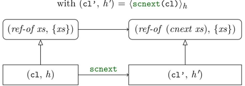
1.3.3.2 Refinement for cnext

The functionscnext defined in Listing 1.6 refines cnext (Definition 1.8): def scnext1[A](c1l:SCList1[A]):SCList1[A] = c1l.next

def scnext[A](cl:SCList[A]):SCList[A] = cl match {

case SCEmpty => SCEmpty

case SCCons(c1l) => SCCons(scnext1(c1l)) }

Listing 1.6: Scala – Definition of scnext1andscnext: returns the cyclic list shifted by one element forwards

with (cl’, h0) = hscnext(cl)i_h

(ref-of xs, {xs}) (ref-of (cnext xs), {xs})

(cl, h) scnext (cl’, h0)

Figure 1.5: Simulation for the refinement of cnext toscnext

This function also uses an auxiliary functionscnext1on non-empty cyclic lists. However,

it appears that its specification is the same as the one for scnext, i. e. cnext. Then its relation would be exactly the one in Figure 1.5.

Proof outline for Figure 1.5. Similarly as Figure 1.3, the first relation (on scnext1) can be proved from the representation of the cyclic list with xs. Yet the fact that the resulting list is still allocated in the heap is not obvious – but still straightforward – as there are transfers between the two parts of the representations: the lists and the additional predicates (describing the pointer closing the cycle) of the initial and final refinement relation.

This relation can be proved by a case distinction on xs.

1.3.3.3 Creating cyclic lists

The previous functions are nice but useless if we can’t construct cyclic lists. We can already contruct empty lists on both levels with [] andSCEmpty, and we naturally have a datatype that should allow to construct non-empty ones but we have to note an oddity that appears as soon as we try to construct a non-empty cyclic list. Indeed a cyclic data structure needs

to reference itself in the same time it is constructed. Therefore there is no way to construct it atomically unless we define it recursively – in which case the language needs to support the recursive definition of values (like OCaml [142]) or to be lazy to avoid non-termination. It is also possible to do it non-atomically by constructing a non-cyclic mutable data structure before, and update it afterwards to point to itself.

This is a general problem encountered as soon as the constructed data structure need to be cyclic. When the cyclicity is not enforced by its type, any terminal value can be used in a first place to be replaced afterwards. When the cyclicity is enforced by the type system, it is harder: as an update can’t change the type of its target, the type of the cyclic data structure needs to be the same as the acyclic one. Thus without an operation offering an atomic construction of a cyclic structure, this is prevented by the type system unless we find a workaround to trick it during the initialization of the construction.

In imperative languages and particularly in Scala, a solution is provided by the null value which can have the type of any reference –AnyRef in Scala – and that we will use only

for temporary assignments. Indeed a general solution is to put an undefined value with the correct type to fill the place of the cycle until we replace it with the correct value.

This is the solution generally used that we will follow for the definition of scsingle1

(used in scsingle) in Listing 1.7. These functions construct a cyclic list containing only one

element.

def scsingle1[A](v:A):SCList1[A] = {

val c1l = new SCList1(v, null) c1l.next = c1l

c1l }

def scsingle[A](v:A):SCList[A] = SCCons(scsingle1(v))

Listing 1.7: Scala – Definition of scsingle1and scsingle: creates a cyclic list containing a single value

On the specification level, we define the function csingle:

Definition 1.14 (csingle)

definition csingle :: 0r ⇒ 0a ⇒ (0r , 0a) clist where csingle r x = [(r , x)]

This one could also be expressed as λr v. cins (r , v) cempty, but as we already said, we prefer the equivalent but clearer list notation.

Here, we note that the reference need to be provided to construct the list. Indeed, it allows to delay the problem of the reference creation from the time of the specification level to the time of the refinement proofs. In the implementation, the reference is furnished by the heap which ensures it will be distinct from the others. Then at the time of the refinement proofs, we will better know the needs and the heap will be available to easily obtain the created reference. We rely on the user of the specification which can provide this new reference by any means, which means this solution is modular. Another solution could have been, for example, to take the heap as argument and use it to generate the new reference (with a primitive Ref-new defined on this heap):