Effect of shell structure on the nucleon transfer contribution to the imaginary part of the heavy ion optical potential

Effect

of

shell

structure

on

the nucleon

transfer

contribution

to

the imaginary

part

of

the

heavy ion

optical

potential

Fl.

Stancu

Institute

_of

Physics, University

of

Liege',

B

40-00 Li'ege _1,Belgium

D. M.

Brink

Theoretical Physics Department, University

_of

Oxford, Oxford OX13ÃP, United Kingdom

(Received 5August 1985)

We calculate the imaginary part ofthe heavy ion optical potential at the strong absorption radius

assuming that the absorption is essentially given by the depopulation ofthe entrance channel due to

nucleon transfer. The transfer probabilities ofindividual nucleons between specific quantum states are calculated with a simple formula. The method is applied toseveral pairs ofnuclei and the

re-sults are compared tothe experiment and other previous calculations.

I.

INTRODUCTION

In the present work we calculate the imaginary part

of

the heavy ion optical potential at the strong absorption ra-dius. As pointed out by Broglia, Pollarolo, and Winther, ' the nucleon transfer process is the dominant mechanism for describing the tail

of

the imaginary part.

Using such an argument in aprevious paper, we calcu-lated the imaginary part W«,

„,

of

the optical potential be-tween various pairs by using the proximity method and a Fermi gas model for describing the interacting nuclei. In this way we could calculate the flux

of

nucleons tunneling through the barrier formed between the single particle wells. All Coulomb effects were neglected. More recent-ly the use

of

the proximity method was formally justified by deriving the definition

of

W„,

„,

used in

Ref.

2 from the transfer probabilities between specific quantum states. The major approximations in relating

8;„„,

to the sum

of

the transition probabilities were that the nuclei are lep-todermous and that their relative motion can be described in a semiclassical approximation by a straight line trajec-tory.

In the present work we study explicitly the effect

of

the nuclear structure on the nucleon transfer contribution to the imaginary part. The study is very similar to that

of

Ref.

4 for

W„,„„where

the shell structure

of

the interact-ing nuclei is taken into account but the method is simpler for numerical calculations. The disadvantage is that it is valid only for large separations between nuclei. On the other hand, it can be easily applied to any pair

of

nuclei. The simplification is due to two main assumptions: (i) The transfer is a peripheral process (the implications

of

this assumption are discussed in the next section). (ii) The protons and neutrons give identical contributions, as in the proximity method. This will allow us to compare the present results with those

of Ref.

2, which gave good agreement with data.

In the next section we shall derive the formula for In Sec.

III

we present numerical results for vari-ous pairs and make a comparison with experiment and

other theoretical estimates. Section IV is devoted to dis-cussion and conclusions.

II.

THEFORMALISM

We assume that the origin

of

coordinates is located in the center

of

the target, called nucleus

2.

The projectile, nucleus 1, moves on a straight line along the y axis with uniform velocity u. The distance

of

closest approach z

=

d is reached at t

=

0.

The transition amplitude

2

(2f,

li) of

a nucleon from a bound state p&;

of

the

pro-jectile to abound state _$2f

of

the target is given perturba-tively by

] 00

3

(2f,

li)=

.

f

(ging, V(g(;

)dt,

(2.1)

(2.2) which does not contain single particle potentials any more. This is the basic formula used to evaluate the imaginary optical potential

8;„„,

which can be related to the total transfer probability

Pb,

—

—

g

~A

(bf, ai)

~

(a,

b

=1,

2) (2.3)

through the relation'

00

W«,

„,

[R(

t)

]dt

=

Pz,

+

P,

z,

(2.4) where

R

isapoint on the trajectory

where V~ is the single particle potential

of

nucleus

1.

For

a peripheral collision this amplitude can take a simpler form.

If

the separation distance is large enough one can find a plane surface X at z

=zo

between the nuclei where both the single particle potentials Vl and V2 can be

neglected for all points ( yx,z )oat any time

t

In such

a.

case

2

(2f, li)

can be rewritten in terms

of

a surface in-tegral over X

&(2f,

li)=

.

f

dt

f

dS(p2fV pf/

fjtV$2f)

R=d+vt

.

(2.5)

~=(k',

+y,

'

)'"=(k', +y,

'

)'"

(2.17) In order to obtain an analytic expression for

8;„„,

com-patible with

Eq.

(2.4) we have to introduce explicitly the single particle wave functions _{1((; and 1(zf}in

Eq.

(2.2).

If

y;

and

_qf

are the eigenstates

of

the nucleus 1and 2at rest corresponding to eigenvalues e; and

_ef,

respectively, one has

which is independent

of

k„and

which will beused below. The transition probability from a specific orbit I; in nu-cleus 1 to a specific orbit lf in nucleus 2 is obtained by summing the square modulus

of

(2.16) over

I;

and

mf.

Making use

of

the addition theorem

of

spherical harmon-ics,we get (i/R)[mv r

.

e;

—

t

—

(1/2)mv t]

„.

=qr;jr

—

R

t je

—(i/fi)e t P2f 9

f(r)e

(2.6) (2.7)

Pl

li,2lf

2I;+1 2lf+1

At this stage we introduce the double Fourier transform

f~(k„,

kz,

z)=

f

e

"

+

""y~(x,

_{y, z)dx} dy (2.8) for

a=i,

f.

It

can be shown that

if

zis outside the range

of

the single particle potentials, expression (2.8)becomes

(

'd

x

f"

dk„

f"

dk„'

(2.18)

f;(z)=C;e

r("

'

Yt(fc(,

) for

a=i

y

i™i

(2.9) where

ff(z)=Cfe

'

Yt

~

(k2) for

a=f,

y

f f

(2. 10)

where C are normalization constants (see the Appendix) and

ki

ki

—

—

2

(k„k„'+ki+yy'),

Voi

k,

*

k,

'=,

(k„k„'+k,'+yy')

.

Vof (2.19) y2

=k

2

+ki+yo. =k

2 2 2

+k2+yof

2 2 (2.11)

We write the transition probability from nucleus 1 to

nucleus 2 as ]

ki

—

—

(

ik„,

—

—

iki, y);

k2=

(

ik„,

—

ik2,

—

y),

7Oi &Of

2j;+1 2jf+1

(2.20) (2.12)

1 1 2

k)

—

(ef

e;

—

~t)iU ); k2

—

(ef

e;

+

Tmu )

A'v '

'

' Av (2.13) 2@i 3'oa=

—

&a

.

Q2 (2.14) .

X

f((k»k

(,zo

d),

(2.

15)—

I

Returning to

Eq.

(2.2) one can see that only the z com-ponents

of

the gradient evaluated at z

=zo

contribute to the transition amplitude. Byreplacing

_y

with the inverse Fourier transform

of

(2.8) and making the derivative with respect toz

of

(2.9)and (2. 10) one obtains at z

=zo

A

_(2f,

1i)

=

i'

1

f

dk„y

ff*(k„,

k2,zo)

plv 2w

This equation contains a number

of

approximations: (i) We assume that neutrons and protons contribute equally to P&2. The sum is taken only over neutron states and the factor 2accounts for the proton contribution. (ii) Actual-ly the transition takes place from levels

_j;l;

to levels

jf1f.

The factors

(2j;+1)

and

(2jf+1)

are the degeneracies

of

the

j

levels and occur because we assume that the initial levels

_j;

are full and the final levels

jf

are empty (iii) Ex. -pression (2.20) contains an implicit dependence on

_j;

and

jf

through the binding energies e; and

ef.

We include this effect by allowing the normalization coefficients C; and

Cf

and go; and @of to be

j

dependent. There are other spin-dependent effects which are neglected

One can evaluate numerically the double integral in (2. 18) but it is interesting to go a step further with the analytical expression.

If

we use the approximations

or using the explicit forms (2.9) and (2.10) the transition amplitude from 1to 2 becomes

e

A

(2f,

li)

=i

C;Cf

f

dk„Yt'~

(k2) (2. 16) A similar expression for the transfer

of

nucleons from the target to the projectile can be obtained by interchanging

i

and

f

in (2.16). _{We notice that y} is a function

of

k„,

as defined in

Eq.

(2.

11).

We introduce the quantity

1 2

=

1 2

y=g+

k,

y'=g+

k'

2'

2'

1 1

yy'

and make the change

of

variables

x

=k„—

k„';

X'=

—,'

(k„+k„')&dig,

expression (2.18) becomes

(2.21)

m

I

11,2l 2 mv ,2 (2li

+

1 )(2I

_f

+

1)ICi Cy I

'

V=

_Vpf(p)

+

Vh1'Srp

f

(p) q1 d

r

dr where (3.1) where e

—

21ld M11

gd

(2.23)

f

_(r)

₌

_1+exp

₍₃₂₎

Mii

—

—

I

dXe

Pi(A;+BiX

)

In order tobe able tomake a comparison with the prox-imity results we choose the parameters in Eqs.

(3.

1)

—

(3.

2) from Bohr and Mottelson as in

Ref.

2,

with

XPi

_(Ay+aX

),

(2.24) VO

—

—

—

50 MeV, Vls

=22

MeV;

r0

—

—

1.

25, a

=0.

65 fm,

R

=F03

'.

(3.3) 2kl

A;=1+

_2;

B

YOi +QOi

2k,

'

Af

—

—

1+

2 ',

Bf—

3of

~70f

(2.25)

Approximation (2.23) has been tested numerically and found tobeaccurate within

1%.

The interesting point about (2.23)is that itshows an ex-plicit exponential decrease

of

the transition probability and ithints at a similar behavior for

W„,

„,

. This helps us to find an expression for W«,

„,

compatible with (2.4). Expression (2.23) suggests that each transition will give rise to an absorptive potential

of

the form

W«,

»(R)

—

Wpe (2.26)

Around the point

of

the closest approach one can take

v2t2

R=d

1+

2d2 (2.27)

(d)

=

v Q~'irdI _ll,

21~.

(2.28) where we have assumed

W '

~(d)=W

(2.29)

The quantity g depends on the specific transition, as we shall see in the next section. The imaginary part

of

the optical potential at the strong absorption radius d

=DI~2

will be calculated as

W«,

„,

(d)

=

g

[

W,",

,

_„,

~(d)+

W„',

_„,

'~(d)]

.

i,

f

(2.30)

III.

RESULTS

The essential ingredients

of

our calculations are the sin-gle particle spectra and the normalization constants C~

of

the asymptotic wave functions

of

the associated orbits in the initial

a

=i

and the final

a

=

f

nuclei.

Each nucleus is described by a single particle potential

of

the form

and using it together with (2.26) one can solve the integral on the left-hand side (lhs)

of

(2.4), This brings us

to

the following form for the absorptive potential at the strong absorption radius

d:

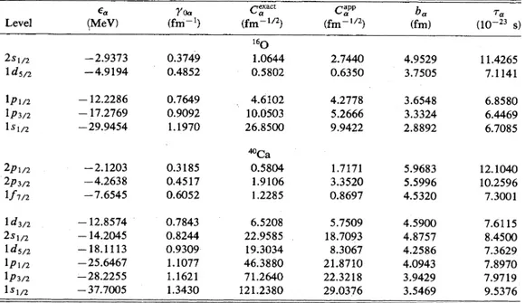
The single particle energies for zS, pNi, and p8pb _and

the corresponding normalization constants

C

are given in Table

I.

The

C

can also be calculated in the approxi-mation described in the Appendix.

Our results are summarized in Table

II.

The pairs

of

nuclei chosen for this study are common either with

Ref.

2or

Ref.

4. As a general trend we notice that the present method gives values at the strong absorption radius for

W«,

„,

close to those

of

Pollarolo et al. On the other hand, they are usually smaller than those obtained with the proximity method, where nuclei are treated in a Fermi gas model. This indicates that the shell structure plays a very important role. In order to see how this effect ap-pears we give in Table

III

the detailed contribution

of

each transfer taking place between the pair '

0+

Ca at

Ei,

b

—

—

74.4 MeV (Digp

—

—

9.

3 fm) and

Ei,

b——

214.

1 MeV

(D&&z

—

—

8.

8 fm).

For

each transfer we also indicate the

value

of

g.

Equation (2.23) for the transfer probability contains a factor exp(

—

2gd), where d is the separation distance between nuclei and q is given in

Eq.

(2.17). Us-ing (2.13) and (2.14) one can rewrite (2.17) as

,

[(&y

—

&;)'+(

—,'mv )

]

—,

(ey+e;) .

(3.4)

The transfer probability is very sensitive to the value

of

g.

One can see that a small _Q value (Q

=e~

—

e;) at fixed v

favors smaller values

_{of g}

and, accordingly, larger values

of

the transfer probability. This is why levels closest to the Fermi surface usually contribute most _{to W«,}

_».

quantity

_g

also enters the integral (2.24) through the argu-ments (2.25) and can give a substantial modification to the exponential term in (2.23). The C; and C~ in the same equation are sensitive to the binding energy and angular momentum

of

the corresponding orbits (Table V) and can amplify ordiminish the transition probability.

Table

II

shows several examples

of

the energy depen-dence

of

W«,

».

We found that it increases in strength with increasing bombarding energy. The single transition values given in Table

III

show that more channels contri-bute at higher energies. The same pattern occurs in the other cases. Our examples are in the range where for each pair

of

levels _g decreases with increasing energy. This is not always the case. Equation (3.4) shows that for high energies, _g increases with v.

The dependence on

_g

also implies a sensitivity

of

the nucleon transition probability on the single particle

spec-O &D E~& 5a

&o

I

~

eh ~W _Q M O W m O 05 (Q_Pl Q crt O o o O cP CP 46 05 OQ ~W _Q

g

O ~N 05 ~~ 0$ O pH cd tQ o

~

~8

~ %~~I cd +& G4

~

O ~a ~~ Cti

c

~

O & O cd

~

O g O cd ~8+4 OOOO~MOO

O&t

Oct

OO m

nQnQ

C O Ch O W Q Ch OO O OO OO cV Ch O cu hp

~

Ch OO O O OO

~

Ch O

e

OO O t OO OO t t Ch C&

OOOO

oa OO I I I I I I I I i I l

AOO

O t t Ch O O Ch t OO OO Q O t OO LO

8

Ch

™

V) ~~ O O OO M rt O

oOOOO

OO Ch O rt. W O OO t OO OO I O Ch O

~

O rt O

~

Ch M O I I I I I I I I Q OO OO

~

OO VO O OO VO m OO t OO Ch VO

OOe~O

I I I I I I I I I I I I I I

trum associated with each reaction partner. In other words, the results are expected to be sensitive to e; and

ef

of

each specific channel through the difference

Q

=

E;

—

e'f as well as through the sum e;

+

ef,

as seen from

Eq.

(3.4). Inorder to have an idea

of

the dependence

of

the results on the choice made for the single particle spectrum, we give in Table IV the values

of

the imaginary potential W,",~„',for '

0+

Pb obtained with the experi-mental single particle spectrum (esps) taken from

Ref.

9.

The separate contributions from

0

—

+Pb and

Pb~O

are also indicated. In these calculations the normalization constants

C

have been evaluated according to the ap-proximation described in the Appendix and are based on the standard average potential

(3.l)

—

(3.5) but taking

Vg,

—

—

0.

The remaining columns in Table IV show the

corresponding quantities

8"

calculated with theoretical single particle energies.

To

make a better comparison we have used

O'

P_{obtained by the approximate method. The}

same number

of

transitions are included in both cases. In contrast, the values in Table

II

included contributions from three deeper levels _{1h»&2, 3s&~2,} and 2d3/2 which are not known experimentally. One can see that for all energies the transfer

Pb~O

isby far the dominant contri-bution to

8",

_,

',

"„'„while

in

8",

_,

","„, the

O~Pb

and

Pb~O

transfers contribute more similarly. This change is due to the fact that the experimental occupied single particle spectrum is higher in energy than the theoretical one in

Pb and lower in ' O. The effect is especially pro-nounced _{at E»b}——_129.5MeV.

Finally the largest value

of

8,

',

",

_„,

in Table

II

is for '

_O+

_{Ni. This is because Ni is not a closed shell} nu-cleus. The shell effects are therefore less important and the result is closer to the proximity value than for all the other cases. The same holds forthe system S

+

S.

IV. CONCLUSIONS

We have calculated the nucleon transfer contribution to the imaginary part

of

the heavy ion optical potential by a method which takes account

of

shell effects. Gur results for the absorptive potential at the strong absorption radius are systematically smaller than those obtained with the proximity method which uses a Fermi gas model. This comparison shows that shell structure plays an important role in the depopulation

of

the entrance channel.

Our potentials are also smaller than those fitted to ex-perimental data. This is not surprising, as the contribu-tion

of

inelastic channels has been neglected. The results

of Ref.

4 show that this contribution can be important.

For

example, the inelastic and transfer channels are both significant for '

0+

Pb at E»b

—

—

192 MeV.

Sometimes very few transitions contribute to

8

trans. In

the case

of

the pair '

0+

Ca at E»b

—

—

40MeV there is only one. _{At E»b}

—

—

214.

1 MeV five transitions make a significant contribution (cf.Table

III).

This illustrates a general trend. At high energies more transitions are im-portant. The energy dependence is influenced strongly by the factor exp(

—

2gd) in

Eq.

(2.23). This factor isa max-imum when

_g

is as small as possible. In all the cases we have studied _q decreases with increasing energy. Typical values for the dominant transitions have _g values lying in

TABLE

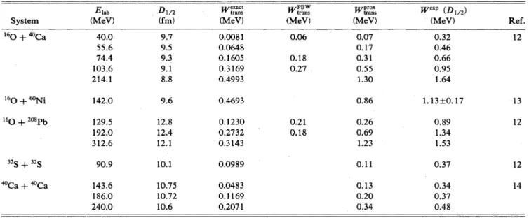
II.

The absorptive potential due to transfer channels. D1/2

—

the strong absorption radius; 8"„",'„",

—

the present result;

S'„,

„,

—

from Ref.4;

8't,

",„",

—

from Ref.2;

8""P

—

the value ofthe phenomenological potential at the strong absorption radius taken from the references indicated in the last column.

System 16O

₊

40Ca Elab (MeV) 40.0 55.6 74.4 103.6 214.1 D1/2 (fm)

9.

7

9.

5 9.3 9.1 8.8 inexact_ii trans (MeV) 0.0081 0.0648 0.1605 0.3169 0.4993 ~PBW trans (MeV) 0.06 0.18 0.27 ugprox ii trans (MeV) 0.07 0.17 0.31 0.55 1.30 ~exp (MeV) 0.32 0.46 0.66 0.95 1.64 Ref. 16o

₊

60Ni 16Q

₊

208Pb 142.0 129.5 192.0 312.6

9.

6 12.8 12.4 12.1 0.4693 0.1230 0.2732 0.3143 0.21 0.18 0.86 0.26 0.69 1.23 1.13+0.17 0.89 1.34 1.53 13 12 32S

₊

32S

Ca+

Ca 90.9 143.6 186.0 240.0 10.1 10.75 10.72 10.6 0.0989 0.0483 0.1169 0.2071 0.11 0.13 0.20 0.34 0.37 0.34 0.37 0.48 12 14

the range

0.

7

—

1 fm

'.

This corresponds to a surface dif-fuseness

a=0.

5

—

0.

7 fm, consistent with the proximity values in

Ref.

2.

For

agiven e;the maximum value

of

_g occurs when

ef

—

—

e;+

—,1

IU

showing that transitions to the continuum can be signifi-cant when the incident energy per nucleon at the Coulomb

barrier (—,' mu )is

of

the order

of

orlarger than the

separa-tion energy Ie'I i

(=10

MeV).

For

such energies it will

not be a good approximation to neglect continuum levels. We note that the proximity method

of Ref.

2 treats bound and continuum levels _{on the same footing. The proximity} method should continue to give a reasonable approxima-tion to

8'„,

_„,

even at high energies when the continuum is important.

TABLE

III.

Detailed contribution ofthe transitions considered in the calculation ofthe imaginary

potential for '

0+

Ca at E1,b

—

—

74.4 and 214.1 MeV. For each transition we indicate the value of

g

—

Eq. (3.4), and the contribution tothe imaginary potential calculated with C~""'

—

Eq.(A2). Transition

O Ca

&Pi/2-&f7n -2p3/2 2p1/2 173/2-1 f7/p -2p3/2 -2p Ca O 1d3/2-1d -2s 2$1/2-1d5/2 -2$1/2 1d5/2"1d5/2 -2$1/2 1p1/2 1d5/2 -2$1/2 1p3/2 1d5/2 -2S1/2 1s1/2-1d5/2 -2s1/2 0.7786 0.8544 0.9302 1.5944 1.1666 1.2652 0.8710 0.9390 0.9501 1.0254 1.1913 1.2817 1.6826 1.7885 1.8547 1.9638 2.4955 2.6125 E1,b

—

—

74.4 MeV ~0-C 0.059206 0.003532 0.000126 0.048211 0.000248 0.000005 exact

'c,

o 0.024 842 0.000226 0.013273 0.000047 0.006 515 0.000010 0.000002 4.

3~

10-"

6.

4~10-'

8.3&&10-" 4.

2~

10 1.2&&

10-"

0.7943 0.7718 0.7656 0.9105 0.9114 0.9189 0.7911 0.7853 0.8265 0.8244 0.9334 0.9405 1.1521 1.1716 1.2294 1.2521 1.5203 1.5518 E1,b

—

—

214.1 MeV exact

~o-c.

0.064865 0.011077 0.001203 0.181401 0.011468 0.001035 0.042 559 0.001 304 0.089152 0.002561 0.076662 0.001 042 0.005635 0.000026 0.009164 0.000031 0.000127 0.000001

TABLE IV. Compalison between results forthe imaginary potential of'

0

+

Pb obtained with the experimental single particle spectrum $f' P' _{and with the theoretical spectrum W'PP. Separate contributions from transitions}

₀

_—

+Pb and

Pb~O

are indicated

(seethe text fordetails). Inallcases the normalization constants C'Pp

—

_{Eq. (A8)}

—

_{are used.}

Elab (Mev) 129.5 192.0 312.6

+

I/2 (fm) 12.8 12.4 12.1 esps +'O Pb 0.0021 0.0180 0.0354 esps ~Pb O 0.3248 0.3710 0.2552 rszesps r' trans 0.3269 0.3890 0.2906 Wg pb 0.0336 0.0778 0.0864 0.0718

'0.

1420 0.1240 mapp « trans 0.1054 0.2198 0.2104 ACKNO%'LEDGMENTS

We would like to thank

L.

Lo

Monaco for discussions, for checking some

of

our results, and for help in calculat-ing normalization constants. One

of

us

(F.S.

)

acknowl-edges financial support from the Science and Engineering Research Council

of

the United Kingdom and kind hospi-tality offered by Peter Hodgson at the Nuclear Physics Department

of

Oxford University.

APPENDIX

In this appendix we recall the definition

of

the asymp-totic normalization constants

C

and derive an analytic approximation which can be used for estimating them with apocket calculator. We introduce

R (r)

as the radi-al part

of

the eigenstate y~(r) normalized such as

f,

~R (r)

~'«=1.

(A1)

The quantity

C

is defined as the normalization constant

of R

outside the range

of

the single particle potential. In this region R can be represented by a spherical Bessel function

hi'"

of

the third kind' and therefore we can

write

i'C~—

yo~rh~"'(i yo~r) for

V-0

.

The asymptotic form

of

hi"

at very large

r

gives

(A2)

(A4)

R~=C

e (A3)

The function

—

i

h~ '(iyo r) is always positive and we choose by convention to have

C &0

always. The exact value

of

the normalization constant

C~""'

can be found by solving the Schrodinger equation numerically for

_R~

and then extracting it from (A2) at an appropriate range r

In.

this case the index

a

stands for the energy e or equivalently the wave number

_yo,

the angular momen-tum

l,

and the total angular momentum

j

of

the orbit under consideration. Our approximate evaluation

of

the C is based on the Wentzel-Kramers-Brillouin (WKB) ex-pression"

of

the wave function

R~.

If

a and b~ are the inner and outer turning points, one can write

Ca

.

r

R

(r)-

sin

f

_~y

(r')

~«'+

—,

a

«&b

4 '

TABLEV. Comparison between Ca'"'

—

Eq. (A2)

—

and Capp

—

_Eq.(A8)

—

for theoretical single par-ticle levels of 160 and ~Ca.

%e

lndlcate also the blndlng energy 6 the wave number _yo.

—

Eq (214)

the outer turning point

b,

and the half-period ~

—

Eq. (A11). Level 2$ 1d5/2 (MeV)

—

2.9373

—

4.9194 Qoa (fm ') 0.3749 0.4852 ~exact Ca (fm ' ) 160 1.0644 0.5802 C'PP_a (fm ' ) 2.7440 0.6350 b (fm) 4.9529 3.7505 (10 s) 11.4265 7.1141 1_p1/2 1_p3/2 1$1/2

—

12.2286

—

17.2769

—

29.9454 0.7649 0.9092 1.1970 4.6102 10.0503 26.8500 4.2778 5.2666 9.9422 3.6548 3.3324 2.8892 6.8580 6.4469 6.7085 2p1/2 2p3/2 1f7m

—

2.1203

—

4.2638

—

7.6545 0.3185 0.4517 0.6052 Ca 0.5804 1.9106 1.2285 1.7171 3.3520 0.8697 5.9683 5.5996 4.5320 12.1040 10.2596 7.3001 1d3/2 2$1/2 1_d5/2 1p1/2 1p3/2 1$

—

12.8574

—

14.2045

—

18.1113

—

25.6467 28.2255

—

37.7005 0.7843 0.8244 0.9309 1.1077 1.1621 1.3430 6.5208 22.9585 19.3034 46.3880 71.2640 121.2380 5.7509 18.7093 8.3067 21.8710 22.3218 29.0376 4.5900 4.8757 4.2586 4.0943 3.9429 3.5469 7.6115 8.4500 7.3629 7.8970 7.9719

9.

5376

1 Ca

e,

—

m (r)

f)ga,

Va

(A5)

TABLE VI. Comparison between the imaginary potential calculated with

C'

and C~"'" for separate transitions

0~Ca

and Ca

—

+0

atEi,b

—

—

103.6MeV; D&i2——

9.

1fm.

where 2m

(l+

Ti) y

=

yo

+

I'(r)+

r

(A6) Transfer

0~Ca

Ca O LL'aI'I'

"

trans (MeV) 0.0749 0.0877 ~exact trans (MeV) 0.1965 0.1204 1' w

(r)

=

y

(r')dr'

.

(A7)

[

2 b2

+(/

+

)2]1j2

The normalization constants C can be on one hand

relat-ed to

Ca.

From (A3), (A5), and (A7) one obtains for large

[yo.b'.

+(l

+

—,'

)']'"+

i+

—,

—

_(I

₊

—,' )ln

Xo&

e~Oa a a

C

2 V'yo (AS)

—

boa&a (A13)

where

P

E

=

_[yo

y(r')]d—

r';

r~

oo

.

(A9) On the other hand, Ca can be expressed in terms

of

the period

2r

of

the orbit

a.

Bymaking the assumption that the main contribution to the lhs

of

(Al) comes from the interval (a b

a),

one has

b

ya

where we have averaged over the periodical function. By defllllllg ra as pl

Iy

I one obtains 2m 1 (A11) (A12)

One can see now that in order to calculate Ca from the approximation (AS) one must know

r

and

K .

Both these quantities depend on the single particle potential

V(r)

through (A6). At this stage we neglect the spin-orbit part

of

(3.1). Then the

j

dependence

of

r

and

K

will come only through e (or yoa). The half-period

r

is ob-tained by integrating

(All)

numerically. In ICa we make a further approximation, by neglecting also the central part

of V(r).

Extending the upper limit to oo, the in-tegral (A9)can be evaluated with the result

In Table V we show a comparison between

C'""'

ob-tained from solving the Schrodinger equation forthe orbit

a

and

Ca

"calculated from (AS) and (Al1)

—

(A14) for '

0

and Ca. Together with the results for Ca we also repro-duce the values

of

the quantities

_yo,

ba, and ~a used in (AS). We notice that the approximation (A8) takes into account quite well the effect

of

the barrier (i.e., large

values

of

C for l

=0

and smaller values with increasing

l).

The agreement between

Ca""'

and- Ca~~ for orbits around the Fermi level is satisfactory.

For

deeper orbits the agreement worsens because the neglect

of

V(r) is no longer a good approximation, but the transition probabili-ty between these levels is insignificant at the bombard-ment energies considered throughout this study.

For

nu-clei where

C'

"

is sometimes larger or sometimes smaller than

C'""',

a compensation effect can occur in adding up the contributions

of

various transitions. A typical exam-ple is the transfer

Ni~Q

at

El,

b

—

—

142 MeV. But this is

not always the case. In Table

VI

we show results for

W„»,

of

'

0+

Ca at E»b

—

—

103.

6MeV obtained on one hand with

Ca""'

and on the other hand with

Ca".

We notice that

_{Wc, ~}

does not change much but

becomes more than two times larger when

Ca""'

are used. The approximation (A8) is useful when an exact solution

of

the Schrodinger equation is not known.

For

example, transitions between experimental single particle levels can be studied by using experimental energies

e

and by es-timating b and w from the standard single particle po-tential

(3.

1)

—

(3.

3). Values

of

the imaginary potential

8'"~'

_{in Table IVare calculated in this way.}

R.

A. Broglia, G. Pollarolo, and A. Winther, Nucl. Phys. A361, 307(1981).

Fl.Stancu and D.M.Brink, Phys. Rev. C 25,2450(1982). D.M.Brink and Fl.Stancu, Phys. Rev. C 30, 1904 (1984).

Pollarolo, R. A. Broglia, and A. Winther, Nucl. Phys. A406, 369(1983).

5D. M. Brink, Les Houches Lectures, edited by

R.

Balian, M. Rho, and G.Ripka (North-Holland, Amsterdam, 1978), p.4. L.LoMonaco and D.M.Brink,

J.

Phys. G(to bepublished). ~A. Bonaccorso, G. Piccolo, and D. M. Brink, Nucl. Phys.

A441,555(1985).

A. Bohr and

B. R.

Mottelson, Nuclear Structure (Benjamin,

New York, 1969),Vol. 1,Sec. 2-4c. Same asRef.8, but Sec. 3-2.

'oM. Abramowitz and

I.

A.Stegun, Handbook

of

Mathematical Functions (Dover, New York, 1965),p. 437.

llL. D. Landau and

E.

M. Lifshitz, Quantum Mechanics (Per-gamon, New York, 1965), Chap. VII.

G.

R.

Satchler and W.

G.

Love, Phys. Rep. 55,183(1979). G.R.Satchler, Phys. Lett. 58B, 409 (1975).