Dynamic Simulation of Large-scale Power Systems Using a Parallel Schur-complement-based Decomposition Method

Dynamic Simulation of Large-scale Power

Systems Using a Parallel

Schur-complement-based Decomposition Method

Petros Aristidou, Student Member, IEEE, Davide Fabozzi, and Thierry Van Cutsem, Fellow Member, IEEE

Abstract—Power system dynamic simulations are crucial for the operation of electric power systems as they provide important

information on the dynamic evolution of the system after an occurring disturbance. This paper proposes a robust, accurate and efficient parallel algorithm based on the Schur complement domain decomposition method. The algorithm provides numerical and computational acceleration of the procedure. Based on the shared-memory parallel programming model, a parallel implementation of the proposed algorithm is presented. The implementation is general, portable and scalable on inexpensive, shared-memory, multi-core machines. Two realistic test systems, a medium-scale and a large-scale, are used for performance evaluation of the proposed method.

Index Terms—domain decomposition methods, Schur complement, power system dynamic simulation, OpenMP, shared-memory

F

1

I

D

indus-try and academia to check the response of electric power systems to disturbances. Over the last decades, they have become indispensable to anyone involved in the planning, design, operation and security of power systems. Power system operation companies depend on fast and accurate dynamic simulations to train opera-tors, analyze large sets of scenarios, assess the dynamic security of the network in real-time or schedule the day ahead operation. On the other hand, people designing future power systems depend on dynamic simulations to evaluate the proposed changes, whether these involve adding new transmission lines, increasing renewable energy sources, implementing new control schemes or decommissioning old power plants [1].

Complex electric components (like generators, motors, loads, wind turbines, etc.) used in dynamic simulations are represented by systems of stiff, non-linear Differ-ential and Algebraic Equations (DAEs) [2]. Conversely, the network connecting the equipment together is repre-sented by a system of linear algebraic equations. These equations try to describe the physical dynamic character-istics, the interactions and control schemes of the system. A large interconnected system may involve hundreds of thousands of such equations whose dynamics span over very different time scales and undergoing many discrete transitions imposed by limiters, switching devices, etc.

Petros Aristidou is with the Department of Electrical Engineering and Computer Science, University of Liège, Liège, Belgium, e-mail: p.aristidou@ieee.org.

Davide Fabozzi is with the Department of Electrical Engineering and Computer Science, University of Liège, Liège, Belgium.

Thierry Van Cutsemis with the Fund for Scientific Research (FNRS) at the Department of Electrical Engineering and Computer Science, University of Liège, Liège, Belgium, e-mail: t.vancutsem@ulg.ac.be.

Consequently, dynamic simulations are challenging to perform and computationally intensive [1].

In applications concerning the security of the system, for example Dynamic Security Assessment (DSA), the speed of simulation is a critical factor. In the remaining applications the speed of simulation is not critical but desired as it increases productivity and minimizes costs. This is the main reason why power system operators often resort to faster, static simulations. However, opera-tion of non-expandable grids closer to their stability lim-its and unplanned generation patterns stemming from renewable energy sources require dynamic studies. Fur-thermore, under the pressure of electricity markets and with the support of active demand response, it is likely that system security will be more and more guaranteed by emergency controls responding to the disturbance. In this context, checking the sequence of events that take place after the initiating disturbance is crucial; a task for which the static calculation of the operating point in a guessed final configuration is inappropriate [11].

During the last decade the increase of computing power has led to an acceleration of dynamic simulations. Unfortunately, at the same time, the size and complexity of simulations has also grown. The increasing demand for more detailed and complex models (power electronic interfaces, distributed energy sources, active distribution networks, etc.) can easily push any given computer to its limits [1]. However, the emergence of parallel computing architectures resulted in a great boost of the simulation performance. The most prominent parallel algorithms developed are inspired from the field of Domain De-composition Methods (DDMs).

DDM refers to a collection of techniques which re-volve around the principle of “divide-and-conquer”. Such methods have been used extensively in problems deriving from physics and structural engineering [3].

They were primarily developed for solving large bound-ary value problems of Partial Differential Equations (PDEs) by splitting them into smaller problems over sub-domains and iterating between them to coordinate the solution [4]. Following, because of their high effi-ciency and performance, DDMs became popular in DAE problems, such as those appearing in power system simulations, VLSI simulations, multi-domain mechanical design, etc. [5], [6], [7], [8], [9]. In these problems, the so-lution domain refers to the states describing the physics and mechanisms of the underlying process and not to the space domain as usually in PDE problems. A more detailed overview of DDMs is presented in App. A.

In this paper we propose a parallel algorithm for dynamic simulation of large-scale electric power sys-tems based on the Schur complement DDM. A non-overlapping, topological-based, decomposition scheme is applied on large electric power systems revealing a star-shaped sub-domain layout. This decomposition is reflected to a separation of the DAEs describing the system. Following, the non-linear DAE system describ-ing each sub-domain is solved independently by dis-cretizing and using a Newton method with infrequent matrix update and factorization. The interface variables shared between sub-domains are updated using a Schur-complement-based method [8], [10].

The proposed algorithm augments the performance of the simulation in two ways: first, the independent calcu-lations of the sub-systems (such as formulation of DAE system, discretization, formulation of linear systems for Newton methods, solution of linear system, check of convergence, etc.) are parallelized, thus providing com-putational acceleration. Second, it exploits the locality of the decomposed sub-systems to avoid many unnecessary computations and provide numerical acceleration.

Additionally, we present the implementation of the al-gorithm based on the shared-memory parallel program-ming model targeting common, inexpensive multi-core machines. For this, modern Fortran and the OpenMP Application Programming Interface (API) are used. The implementation is general, with no hand-crafted opti-mizations particular to the computer system, Operating System (OS), simulated electric power network or dis-turbance. The results were acquired using four different multi-core computers and show significant acceleration. The paper is organized as follows: in Section 2 we present the power system model formulation and some existing dynamic simulation algorithms. In Section 3, we explain the proposed algorithm and its application on dynamic simulations of electric power systems. In Section 4, some important parallel programming aspects and challenges of the implementation are discussed. Our simulation study is reported in Section 5, followed by a discussion in Section 6 and closing remarks in Section 7.

2

P

S

D

S

Power system dynamic simulations fall in basically two categories: electromagnetic transients and

quasi-sinusoidal approximation. In the former, fast electromag-netic transients are simulated; in steady state, voltages and currents evolve sinusoidally with time at a fre-quency close to the nominal value (50 or 60 Hz). The net-work itself is modeled through the differential equations relative to its inductances and capacitors. On the other hand, in the quasi-sinusoidal (or phasor) approximation, the network is represented through algebraic equations corresponding to sinusoidal regime. During transients, all phasors vary with time while in steady-state they take on constant values [2]. The dynamic model describes how the phasors evolve with time.

The dynamic simulations described in this paper fall in the second category. It is the one commonly used in global stability studies, where the simulated time interval can extend up to several minutes, if not more. Typical time step sizes range form a few milliseconds to seconds.

2.1 Model Overview

An electric power system, under the quasi-sinusoidal approximation, can be described in compact form by the following DAE Initial Value Problem (IVP):

0 = Ψ(x, V) Γ ˙x = Φ(x, V) x(t0) = x0, V(t0) = V0

(1) where V is the vector of voltages through the network,

x is the expanded state vector containing the differen-tial and algebraic variables (except the voltages) of the system and Γ is a diagonal matrix with

(Γ)ℓℓ=

{

0 if ℓ-th equation is algebraic 1 if ℓ-th equation is differential The first part of (1) corresponds to the purely alge-braic network equations. The second part describes the remaining DAEs of the system. This system changes during the simulation due to the discrete dynamics of the system such as response to discrete controls or changes in continuous-time equations. For reasons of simplicity, the handling of these discrete events is not presented in this paper. More details concerning their handling can be found in [11] and its quoted references.

2.2 Review of Solution Algorithms

The existing sequential algorithms can be categorized as partitioned or integrated (simultaneous) [12]. Partitioned algorithms solve separately the differential equations of (1) for the state variables and the algebraic equations for the algebraic variables. Then, these solutions are alternated until convergence. On the other hand, inte-grated algorithms use an implicit integration method to convert (1) into a unique set of algebraic equations to be solved simultaneously. The most popular algorithm in this category [13] is the Very DisHonest Newton (VDHN) detailed in App. B.1.

As soon as parallel computers emerged, several algo-rithms trying to exploit the new computational potential

were proposed. These can be mainly classified into fine-grained [14], [15], [16], [17] and coarse-fine-grained [6], [7], [18], [19], [20], [21], [22] parallel algorithms.

A more detailed overview of existing sequential and parallel algorithms in power system dynamic simula-tions can be found in App. B.

3

P

A

This section describes the proposed parallel Schur-complement-based algorithm.

3.1 Power System Decomposition

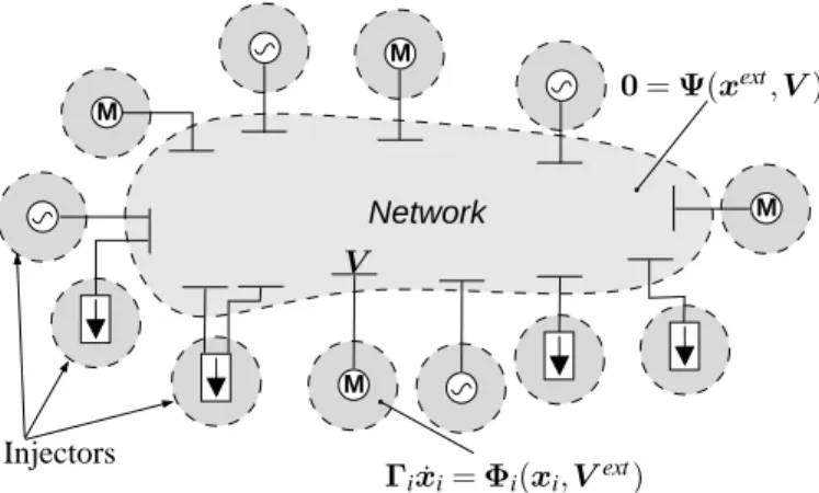
From topological perspective, power systems consist of electric components (e.g. synchronous machines, loads, motors, small distribution network equivalents, etc.) interfacing with each other through the network. For reasons of simplicity, all the aforementioned components connected to the network will be called injectors and refer to devices that either produce or consume power. The proposed algorithm employs a topological decomposi-tion separating each injector to define one sub-domain and the remaining electric network as the central sub-domain of a star layout. The proposed decomposition is visualized in Fig. 1 with each shaded area representing one sub-domain.

This decomposition separates the problem (1) into sev-eral sub-problems, each defined over one sub-domain. Thus, the network sub-domain is described by the alge-braic equations:

0 = Ψ(xext, V)

xext(t0) = xext0 , V(t0) = V0 (2)

while each injector sub-domain i is described by DAEs:

Γi˙xi= Φi(xi, Vext)

xi(t0) = xi0, Vext(t0) = Vext0

(3) where the first N−1 sub-domains are injectors and N-th sub-domain the network. xi and Γi are the projections

of x and Γ, defined in (1), on the i-th sub-domain. Fur-thermore, the variables of each injector xi are separated

into interior xint

i and local interface x ext i variables and Network M M M M Γ_ix_{˙i= Φi(xi} ,V ext₎ 0_{= Ψ(x}ext ,V) V Injectors

Figure 1. Proposed decomposition scheme

the network sub-domain variables V are separated into interior Vint _{and local interface V}ext _variables.

Although for decomposed DAE systems detecting the interface variables is a complicated task [8], for the proposed topological-based decomposition these are preselected based on the nature of the components. For the network sub-domain, the interface variables are the voltage variables of buses on which injectors are physically connected. For each injector sub-domain, the interface variable is the current injected in that bus.

The resulting star-shaped, non-overlapping, partition layout (see Fig. 1) is extremely useful when applying Schur-complement-based DDMs since it allows simpli-fying and further reducing the size of the global reduced system needed to be solved for the interface unknowns. Moreover, the decomposition is based on topolog-ical inspection and doesn’t demand complicated and computationally intensive partitioning algorithms. It in-creases modularity as the addition or removal of injec-tors does not affect the existing decomposition or other sub-domains besides the network. This feature can be exploited to numerically accelerate the solution.

3.2 Local System Formulation

The VDHN method is used to solve the algebraized injector DAE systems and the network equations. Thus, the resulting local linear systems take on the form of (4) for the injectors and (5) for the network.

A1i (resp. D1) represents the coupling between

in-terior variables. A4i (resp. D4) represents the coupling

between local interface variables. A2i and A3i (resp. D2

and D3) represent the coupling between the local

inter-face and the interior variables. Bi(resp. Cj) represent the

coupling between the local interface variables and the external interface variables of the adjacent sub-domains.

3.3 Global Reduced System Formulation

Following, the interior variables of the injector sub-domains are eliminated (see App. A.2.2) which yields for the i-th injector:

Si△xexti + Bi△Vext= ˜fi (6)

with Si = A4i− A3iA−11i A2i, the local Schur

comple-ment matrix and ˜fi= fiext− A3iA−11i f

int

i the

correspond-ing adjusted mismatch values.

The matrix D of the electric network is very sparse and structurally symmetric. Eliminating the interior variables of the network sub-domain requires building the local Schur complement matrix SN which is in general not a

sparse matrix. That matrix being large (since many buses have injectors connected to them) the computational efficiency would be impacted. On the other hand, not eliminating the interior variables of the network sub-domain increases the size of the reduced system but retains sparsity. The second option was chosen as it allows using fast sparse linear solvers.

( A1i A2i A3i A4i ) | {z } ( △xint i △xext i ) | {z } + Ai △xi ( 0 Bi△Vext ) = ( fint i (xinti , xexti ) fext

i (xinti , xexti , Vext)

) | {z } fi (4) ( D1 D2 D3 D4 ) | {z } ( △Vint △Vext ) | {z } + D △V ( 0 ∑N−1 j=1 Cj△xextj ) = (

gint_(Vint_{, V}ext₎

gext_(Vint_{, V}ext_{, x}ext₎

) | {z } g (5) ( D1 D2 D3 D4− ∑N−1 i=1 CiS−1i Bi ) | {z } e D ( ∆Vint ∆Vext ) | {z } ∆V = ( gint gext−∑N_i=1−1CiS−1i ˜fi ) | {z } eg (8)

So, the global reduced system to be solved, with the previous considerations, takes on the form:

         S1 0 0 · · · 0 B1 0 S2 0 · · · 0 B2 0 0 S3· · · 0 B3 .. . ... ... . .. ... ... 0 0 0 · · · D1D2 C1C2C3· · · D3D4                   △xext 1 △xext 2 △xext 3 .. . △Vint △Vext          =          ˜ f1 ˜ f2 ˜ f3 .. . gint gext          (7)

Due to the star layout of the decomposed system, the resulting global Schur complement matrix is in the so called Block Bordered Diagonal Form (BBDF). Manipu-lating this structure, which is a unique characteristic of star-shaped layout decompositions, we can further elim-inate from the global reduced system all the interface variables of the injector sub-domains and keep only the variables associated to the network sub-domain [23].

This results in the simplified, sparse, reduced system (8) where the elimination factors CiS−1i Bi act only on

the already non-zero block diagonal of sub-matrix D4

thus retaining the original sparsity pattern. System (8) is solved efficiently using a sparse linear solver to acquire

V and the network sub-domain interface variables are backward substituted in (4), thus decoupling the solution of injector sub-domains. Then, the injector interior (xint

i )

and local interface (xext

i ) variables are computed and

the convergence of each sub-domain is checked using an infinite norm on its normalized state vector corrections. The solution stops when all sub-domains obey the con-vergence criteria, thus the non-linear systems (3) have been solved.

Other power system decomposition algorithms, like diakoptics [5], use a Schwartz-based approach (App. A) to update the interface variables. This is reflected into an equivalent system of (7) which, instead of BBDF, is in lower/upper triangular form. On the one hand, this form augments the algorithm’s parallel performance by providing fewer synchronization points. On the other hand, it increases the number of iterations needed to converge as the influence of neighboring sub-domains is kept constant during a solution.

Although Schwartz-based algorithms are very use-ful when considering distributed memory architectures

(where the cost of data exchange and synchronization is high), in modern shared-memory architectures the use of Schur-complement-based algorithms, as the one proposed, can compensate for the higher data exchange with less iterations because it retains the equivalent BBD structure of the final matrix.

3.4 Computational Acceleration

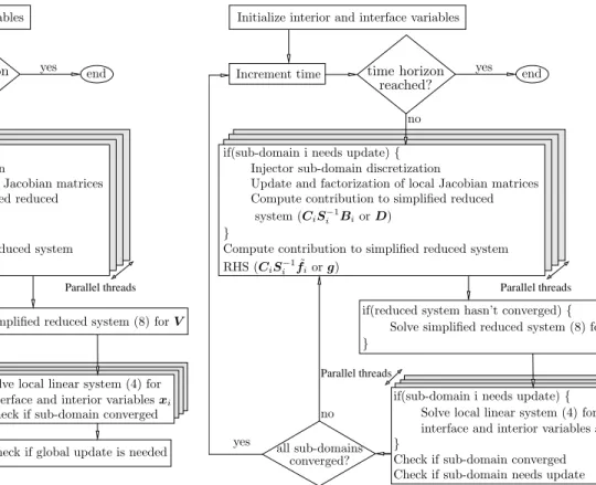
The proposed parallel algorithm -denoted (P)- is pre-sented in Fig. 2. As described above, the VDHN method is used for the solution of the sub-domain systems, thus updating and factorizing the local matrices is done infre-quently. If the decomposed algorithm does not converge after a given number of sub-domain VDHN iterations, then, all the local sub-domain matrices are updated and factorized, the local Schur complement and elimination factors are recomputed and the simplified reduced sys-tem (8) reformulated.

Thus, the main sources of parallelism of the proposed algorithm are the formulation and update of the sub-domain local systems, the elimination of the interior variables and calculation of local Schur complements, the calculation of the elimination factors, the formulation of the reduced system and the solution of the sub-domain systems. These can be seen in the shaded blocks in Fig. 2. The proposed algorithm, as Schur-complement-based, suffers from the sequentiality introduced by the solution of the global reduced system (8). Because of the high sparsity, the linear nature of the network sub-domain and the infrequent system update, this bottleneck is bounded to 5−8% of the overall computational cost (see App. E.2). Although this sequentiality can be tackled by the use of available parallel sparse linear solvers, the new synchronization points introduced would increase the overhead time and counteract any benefits arising from parallelization. Hence, a powerful but general solver [24] has been used in this work. However, in future devel-opment a customized advanced parallel solver (e.g. [25]) could be used to compute this remaining sequential portion in the most efficient manner.

3.5 Numerical Acceleration

The proposed algorithm can also provide numerical ac-celeration, if we exploit the locality of the sub-domains.

Parallel threads

Parallel threads

Figure 2. Proposed parallel algorithm (P)

This is based on the observation that sub-domains de-scribed by strongly non-linear systems or with fast changing variables, converge slower and need more VDHN iterations, while sub-domains with “low dy-namic activity” converge faster and need less VDHN iterations. We can exploit this in two ways.

First, in algorithm (P) the local matrices and the global Schur complement matrices are computed infrequently but in a synchronized way; when the criteria for global update is reached, all matrices are recomputed at the same time. Taking advantage of the fact that each sub-domain is solved by a separate VDHN method, we can decouple the matrix update criteria and allow local system matrices to be updated asynchronously. In this way, sub-domains which converge fast will keep the same local system matrices for many iterations and time-steps, while sub-domains which converge slower will update their local systems more frequently.

Second, in algorithm (P) all sub-domains need to be solved at every iteration up to global convergence. Conversely, if the convergence check is done locally on each separate sub-domain, then many sub-domain solutions can be saved. That is, at a given iteration not-converged sub-domains will continue being solved, while converged sub-domains will stop being solved.

Based on algorithm (P) and the two above enhance-ments, the enhanced parallel algorithm (EP) is presented in Fig. 3. Both algorithms have the same parallelization opportunities but the second algorithm (EP) offers some further, numerical acceleration [11].

Parallel threads

Parallel threads

Figure 3. Proposed enhanced parallel algorithm (EP)

4

P

I

The main reason for applying parallelization techniques is to achieve higher application performance, or in our case, reduce simulation time. This performance depends on several factors, such as the percentage of paral-lel code, load balancing, communication overhead, etc. Other reasons, which are not considered in this paper, include the existence of proprietary data in some sub-domains or the usage of black-box models. In such cases, the method can work if the sub-domains are solved separately and only the interface values are disclosed.

Several parallel programming models were considered for the implementation of the algorithm (see App. C.1). The shared-memory model using OpenMP was selected as it is supported by most hardware and software ven-dors and it allows for portable, user-friendly program-ming. Shared-memory, multi-core computers are becom-ing more and more popular among low-end and high-end users due to their availability, variety and perfor-mance at low prices. OpenMP has the major advantage of being widely adopted on these platforms, thus allow-ing the execution of a parallel application, without any changes, on many different computers [26]. Moreover, OpenMP provides some easy to employ mechanisms for achieving good load balance among the working threads; these are detailed in App. C.2.

4.1 Parallel Work Scheduling

One of the most important tasks of parallel program-ming is to make sure that parallel threads receive equal

amounts of work [26]. Imbalanced load sharing among threads leads to delays, as some threads are still working while others have finished and remain idle.

In the proposed algorithm, the injector sub-domains exhibit high imbalance based on the dynamic response of each injector to the disturbance. In such situations, the dynamic strategy (App. C.2) is to be preferred for better load balancing. Spatial locality can also be addressed with dynamic scheduling, by defining a minimum num-ber of successive sub-domains to be assigned to each thread (chunk). Temporal locality, on the other hand, cannot be easily addressed with this strategy because the sub-domains treated by each thread, and thus the data accessed, are decided at run-time and can change from one parallel segment of the code to the next. When executing on Uniform Memory Access (UMA) architecture computers, where access time to a memory location is independent of which processor makes the request, this strategy proved to be the best.

On the other hand, when executing on Non-Uniform Memory Access (NUMA) architecture com-puters (App C.3), a combination of static scheduling (App. C.2) with a proper choice of successive itera-tions to be assigned to each thread (chunk), proved to provide the best performance. A small chunk number means that the assignment of sub-domains to threads is better randomized, thus practically providing good load balancing. A higher chunk number, as discussed previously, allows to better address spatial locality. So, a compromise chunk size is chosen at runtime based on the number sub-domains and available threads. The same static scheduling and chunk number is used on all the parallel loops, which means that each thread handles the same sub-domains and accesses the same data, at each parallel code segment thus addressing temporal locality.

4.2 Ratio of Sub-domains to Threads

In several decomposition schemes, the number of sub-domains is chosen to be the same as the number of available computing threads and of equal size in order to utilize in full the parallelization potential. Further partitioning is avoided as increasing the number of sub-domains leads to an increased number of interfaces and consequently higher synchronization cost. On the con-trary, the proposed decomposition suggests an extremely large number of injector sub-domains.

First, due to the star-shaped layout, the injector sub-domains of the proposed scheme have no interface or data exchange with each other except with the network. Thus, the high number of injector sub-domains does not affect the synchronization cost. Second, groups (chunks) of sub-domains are assigned at run-time to the parallel threads for computation, thus better load-balancing is achieved as they can be dynamically reassigned. Last, this decomposition permits the individual injector treat-ment to numerically accelerate the procedure as seen in Section 3.5.

These benefits, that is dynamic load balancing and numerical acceleration, cannot be exploited when fewer but bigger sub-domains, aggregating many injectors, are used. In dynamic simulations it is not known which injectors will display high dynamic activity, thus high computational cost, before applying a disturbance. So, to achieve good load balancing the splitting of injectors to sub-domains would need to be changed for each system and applied disturbance. Further, to apply the numerical acceleration presented in Section 3.5, all the injectors of the big sub-domain should be treated at the same time. Hence, the whole big sub-domain should be solved even if only one injector is strongly active.

5

R

In this section we present the results of the Schur Complement-based algorithm implemented in the aca-demic simulation software RAMSES1, developed at the University of Liège. The software is written in standard Fortran language with the use of OpenMP directives for the parallelization.

Three algorithms were implemented for comparison: (I) Integrated sequential algorithm VDHN (see

App. B.1) applied on the original system (1). The Jacobian matrix is updated and factorized only if the system hasn’t converged after three Newton iterations at any discrete time instant. This update strategy gives the best performance for the proposed test-cases.

(P) Parallel decomposed algorithm of Fig. 2. The global update and global convergence criteria are chosen to be the same as of (I).

(EP) Parallel decomposed algorithm of Fig. 3. The local update and local convergence criteria, applied to each sub-domain individually, are chosen to be the same as of (I).

For all three algorithms the same models, algebraization method (second-order backward differentiation formula - BDF2) and way of handling the discrete events were used. For the solution of the sparse linear systems, the sparse linear solver HSL MA41 [24] was used in all three algorithms. For the solution of the dense injector linear systems in algorithms (P) and (EP), Intel MKL LAPACK library was used.

Keeping the aforementioned parameters of the sim-ulation constant for all algorithms permits the better evaluation of the proposed algorithms’ performance.

5.1 Performance Indices

Many different indices exist for assessing the perfor-mance of a parallel algorithm. The two indices most commonly used by the power system community, as proposed in [13], are speedup and scalability.

1. Acronym for “Relaxable Accuracy Multithreaded Simulator of Electric power Systems”.

First, the speedup is computed by:

Speedup(M ) = W all time (I) (1 core)

W all time (P/EP ) (M cores) (9)

and shows how faster is the parallel implementation compared to the fast, well-known and widely used sequential algorithm presented in App. B.1.

The second index is the scalability of the parallel algo-rithm, computed by:

Scalability(M ) = W all time (P/EP ) (1 core)

W all time (P/EP ) (M cores) (10)

and shows how the parallel implementation scales when the number of processors available are increased.

5.2 Computer Platforms Used

The following computer platforms were used to acquire the simulation results:

1) Intel Core2 Duo CPU T9400 @ 2.53GHz, 32KB private L1 and 6144KB shared L2 cache, 3.9GB RAM, Microsoft Windows 7

2) Intel Core i7 CPU 2630QM @ 2.90GHz, 64KB pri-vate L1, 256KB pripri-vate L2 and 6144KB shared L3 cache, 7.7GB RAM, Microsoft Windows 7

3) Intel Xeon CPU L5420 @ 2.50GHz, 64KB private L1 and 12288KB shared L2 cache, 16GB RAM, Scientific Linux 5

4) AMD Opteron Interlagos CPU 6238 @ 2.60GHz, 16KB private L1, 2048KB shared per two cores L2 and 6144KB shared per six cores L3 cache, 64GB RAM, Debian Linux 6 (App. C.3, Fig. 1)

Machines (1) and (2) are ordinary laptop computers with UMA architecture, thus dynamic load balancing was used. Machines (3) and (4) are scientific computing equipment with NUMA architecture, hence static load balancing and the considerations of App. C.3 were used.

5.3 Test-case A

The first test-case is based on a medium-size model of a real power system. This system includes 2204 buses and 2919 branches. 135 synchronous machines are represented in detail together with their excitation systems, voltage regulators, power system stabilizers, speed governors and turbines. 976 dynamically modeled loads and 22 Automatic Shunt Compensation Switching (ASCS) devices are also present. The resulting, undecom-posed, DAE system has 11774 states. The models were developed in collaboration with the system operators.

Table 1

Case A1: Performance summary

average iterations platform (1) (2) (3) (4)

per time step cores 2 4 8 12

(P) 2.6 speedup 1.8 2.1 2.5 3.8

scalability 1.1 1.5 1.7 2.8 (EP) 3.0 _scalabilityspeedup 4.1_1.1 4.5_1.4 4.8_1.4 6.7_2.3

(I) 2.6 - - - -

-The disturbance consists of a short circuit near a bus lasting seven cycles (116.7 ms at 60 Hz), that is cleared by opening two transmission lines (test-case A1). The same simulation is repeated with the difference that six of the ASCS devices located in the area of the disturbance are deactivated (test-case A2). Both test-cases are simulated over a period of 240 s with a time step of one cycle (16.667 ms) for the first 15 s after the disturbance (short-term) and 50 ms for the remaining time up to four minutes (long-term). The dynamic response of test-cases A1 and A2 as well as a comparison on the accuracy of the three algorithms can be found in App. D.1.

Tables 1 and 2 summarize the performance measured for test-cases A1 and A2, respectively. First, the average number of iterations needed for each discrete time step computation is presented. As expected, algorithms (I) and (P) need the same average number of iterations to compute the solution. Conversely, algorithm (EP) requires more iterations as converged sub-domains are not solved anymore and kept constant. However, each iteration of (EP) requires much smaller computational effort, as only non-converged sub-domains are solved, thus the overall procedure is accelerated.

Second, the performance indices achieved on each of the computational platforms. Both parallel algorithms (P) and (EP) provide significant acceleration when com-pared to the sequential algorithm (I). As expected, the best acceleration is achieved by algorithm (EP) which takes advantage of both the computational and numer-ical acceleration as described in Sections 3.4 and 3.5, respectively. It is noticeable that even on inexpensive portable computers (like UMA machines (1) and (2)) a significant acceleration is achieved with an up to 4.5 times speedup. On the bigger and more powerful computers used a speedup of up to 6.7 times is obtained. Moreover, it is worth noticing that test-case A2, which is an unstable case (see App. D.1), requires on average more iterations per discrete time step computation. In fact, as the system collapses (App. D.1, Fig. 3) the injector sub-domains become more active, thus more iterations are needed for convergence. This also explains why test-case A2 shows slightly better scalability. That is, the additional number of sub-domain updates and solutions are computed in parallel, hence increasing the parallel percentage of the simulation (see App. E). At the same time, test-case A2 benefits less from the numerical speedup with algorithm (EP) as more active injector sub-domains delay to converge.

Table 2

Case A2: Performance summary

average iterations platform (1) (2) (3) (4)

per time step cores 2 4 8 12

(P) 3.5 speedup 1.9 2.3 2.6 3.9

scalability 1.2 1.6 1.8 3.0 (EP) 4.2 _scalabilityspeedup 3.8_1.1 4.2_1.4 4.5_1.5 6.2_2.3

-Table 3

Case B: Performance summary

average iterations platform (1) (2) (3) (4)

per time step cores 2 4 8 24

(P) 2.2 speedup 1.4 2.0 2.7 3.9 scalability 1.5 2.1 2.5 3.9 (EP) 2.6 speedup 2.9 3.3 4.1 4.7 scalability 1.4 1.7 1.8 2.9 (I) 2.2 - - - - -5.4 Test-case B

The second test-case is based on a large-size power system representative of the continental European main transmission grid. This system includes 15226 buses, 21765 branches and 3483 synchronous machines rep-resented in detail together with their excitation sys-tems, voltage regulators, power system stabilizers, speed governors and turbines. Additionally, 7211 user-defined models (equivalents of distribution systems, induction motors, impedance and dynamically modeled loads, etc.) and 2945 Load Tap Changing (LTC) devices are included. The resulting, undecomposed, DAE system has 146239 states. The models were developed in collaboration with industrial partners and operators of the power system.

The disturbance simulated on this system consists of a short circuit near a bus lasting five cycles (100 ms at 50Hz), that is cleared by opening two important double-circuit transmission lines. The system is simulated over a period of 240 s with a time step of one cycle (20 ms) for the first 15 s after the disturbance (short-term) and 50ms for the rest (long-term). The dynamic response of test-case B as well as a comparison on the accuracy of the three algorithms can be found in App. D.2.

Table 3 summarizes the performance measured for this test-case. As with test-cases A1 and A2, algorithms (I) and (P) need the same average number of iterations to compute the solution at each discrete time step, while (EP) slightly more. Furthermore, the performance indices show significant acceleration of the parallel algorithms compared to algorithm (I).

The scalability of test-case B is higher than of A1 and A2 as the significantly larger number of injectors

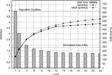
0 0.5 1 1.5 2 2.5 3 3.5 4 4.5 5 5.5 1 2 4 6 8 10 12 14 16 18 20 22 24 0 50 100 150 200 250 300 350 400 450 500 550 600 650 700 750 Speedup Wall time (s) cores Simulated time=240s Algorithm (I)=660s Wall time Speedup Ideal speedup

Figure 4. Case B: Speedup of algorithm (P)

0 0.5 1 1.5 2 2.5 3 3.5 4 4.5 5 5.5 1 2 4 6 8 10 12 14 16 18 20 22 24 0 50 100 150 200 250 300 350 400 450 500 550 600 650 700 750 Speedup Wall time (s) cores Simulated time=240s Algorithm (I)=660s Wall time Speedup Ideal speedup

Figure 5. Case B: Speedup of algorithm (EP)

in the second system provides higher percentage of computational work in the parallelized portion. On the other hand, test-case B exhibits smaller overall speedup (4.7) compared to A1 and A2 (6.7 and 6.2 respectively). This can be attributed to the numerical acceleration of algorithm (EP), better benefiting test-cases A1 and A2. That is, many injectors in test-cases A1 and A2 converge early during the iterations and stop being solved (see Section 3.5), thus the amount of computational work inside each iteration is decreased and the overall sim-ulation further accelerated.

Finally, Figs. 4 and 5 show the speedup and wall time of the algorithms (P) and (EP) when the number of threads on machine (4) are varied between one and 24. The ideal speedup is calculated using the profiling results of the test-case in sequential execution to acquire the parallel and sequential portion (App. E.2) and Am-dahl’s law (App. E.1).

6

D

This section presents a discussion concerning the sequen-tial, parallel and real-time performance of the proposed algorithms executed on NUMA machine (4).

6.1 Sequential Performance

In sequential execution, algorithms (I) and (P) perform almost the same (see Fig. 4, one core). On the other hand, due to the numerical accelerations presented in Section 3.5, algorithm (EP) is faster by a factor of 1.5−2.0 (see Fig. 5, one core). Therefore, the proposed algorithm (EP) can provide significant acceleration even when exe-cuted on single-core machines. Moreover, it can be used on multi-core machines to simulate several disturbances concurrently using one core for each.

6.2 Parallel Performance

Equations 9 and 10 provide the actual speedup and scalability achieved by the parallel implementation. These indices take into consideration the OverHead Cost (OHC) needed for creating and managing the parallel

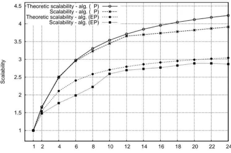
threads, as well as any other delays occurring in the implementation (e.g. due to load imbalances). To assess the performance of a parallel implementation Amdahl’s law can be used [27] to provide its theoretical scalability, that is the theoretical maximum performance of the implementation if no OHC and perfect load balancing is considered. This theoretical maximum can be used to evaluate the quality of an implementation (see App. E). Figure 6 shows how algorithms (P) and (EP) scale over a changing number of cores for test-case B. The theoretic scalability curves are plotted using the profiling results and Amdahl’s law. The difference between the theoretic scalability and the measured scalability is due to costs of managing the threads and communication between them. This is better explained by the modified Amdahl’s law (see App. E.1) which includes the OHC. The spread among theoretic and measured curves can be minimized if the costs of synchronization and communication, and thus OHC, are minimized.

To achieve this, further study on the algorithmic part (merging some parallel sections of the code to avoid syn-chronizations, parallelizing other time consuming tasks, etc.) and on the memory access patterns and manage-ment (avoiding false sharing, arranging better memory distribution, etc.) is needed. Especially for the latter, particularly interesting is the effect of LAPACK solvers used for the parallel solution of sub-domains. These popular solvers do not use optimized data structures to minimize wasting memory bandwidth or minimize conditionals to avoid pipeline flushing in multi-core execution. Techniques have been proposed for the devel-opment of customized solvers [25] to help alleviate this issue and need to be considered in future development. Finally, a slight decrease of the scalability of (EP) is observed when the number of threads exceeds 22 (see Fig. 6). That is, when using more than 22 threads, the scalability degrades compared to the maximum achieved. The degradation occurs as the execution time gained (P

22−

P

24), when increasing from 22 to 24 threads,

is smaller than the overhead cost OHC(24)− OHC(22) of creating and managing the two extra threads (see App. E.1).

6.3 Real-time Performance

Fast dynamic simulations of large-scale systems can be used for operator training and testing global control schemes implemented in Supervisory Control and Data Acquisition (SCADA) systems. In brief, measurements (such as the open/closed status from a switch or a valve, pressure, flow, voltage, current, etc.) are transfered from Remote Terminal Units (RTUs) to the SCADA center through a communication system. These information are then visualized to the operators or passed to a control software which take decisions for corrective actions to be communicated back to the RTUs. In modern SCADA systems the refresh rate (∆T ) of these measurements is 2− 5 seconds [28]. 1 1.5 2 2.5 3 3.5 4 4.5 1 2 4 6 8 10 12 14 16 18 20 22 24 Scalability cores Theoretic scalability - alg. ( P)

Scalability - alg. ( P) Theoretic scalability - alg. (EP) Scalability - alg. (EP)

Figure 6. Case B: Scalability of algorithms (P) and (EP) The simulator in these situations takes on the role of the real power system along with the RTU measurements and the communication system. It needs to provide the simulated “measurements” to the SCADA system with the same refresh rate as the real system. Thus, the concept of “real-time” for these applications translates to time deadlines.

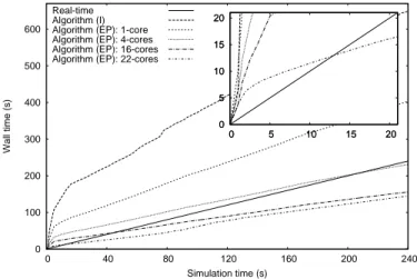
In Fig. 7 we observe the performance of the algorithm for test-case A1. The straight diagonal line defines the limit of faster than real-time performance. When using six or more cores for the simulation, algorithm (EP) is able to simulate any of the tested disturbances on this system faster than real-time throughout the time horizon. That is, all simulation timings lay below the real-time line and all possible time deadlines can be met. On the other hand, in Fig. 8 we observe that test-case B is faster than real-time after the initial 13 s. However, time deadlines with ∆T ⩾ 4 s can still be met as the maximum lag between simulation and wall time is 4 s. Overall, a wide range of available test-systems was evaluated in the same way for their real-time perfor-mance. A model of 8053 buses and 11292 injectors (to-taling 74930 states) was found to be the limit of the proposed implementation, on platform (4), with faster than real-time execution.

0 40 80 120 160 200 240 0 40 80 120 160 200 240 Wall time (s) Simulation time (s) Real-time Algorithm (I) Algorithm (EP): 1-core Algorithm (EP): 6-cores Algorithm (EP): 12-cores

0 1 2 3 4 5 0 1 2 3 4 5 0 1 2 3 4 5 0 1 2 3 4 5

0 100 200 300 400 500 600 0 40 80 120 160 200 240 Wall time (s) Simulation time (s) Real-time Algorithm (I) Algorithm (EP): 1-core Algorithm (EP): 4-cores Algorithm (EP): 16-cores Algorithm (EP): 22-cores

0 5 10 15 20 0 5 10 15 20 0 5 10 15 20 0 5 10 15 20

Figure 8. Case B: Real-time performance (EP)

7

C

In this paper a parallel Schur-complement-based algo-rithm for dynamic simulation of electric power systems is presented. It yields acceleration of the simulation pro-cedure in two ways. On the one hand, the propro-cedure is accelerated numerically, by exploiting the locality of the sub-domain systems and avoiding many unnecessary computations (factorizations, evaluations, solutions). On the other hand, the procedure is accelerated computa-tionally, by exploiting the parallelization opportunities inherent to DDMs.

The proposed algorithm is accurate, as the original system of equations is solved exactly until global con-vergence. It is robust, as it can be applied on general power systems and has the ability to simulate a great variety of disturbances without dependency on the exact partitioning. It exhibits high numerical convergence rate, as each sub-problem is solved using a VDHN method with updated and accurate interface values during the whole procedure.

Along with the proposed algorithm, an implementa-tion based on the shared-memory parallel programming model is presented. The implementation is portable, as it can be executed on any platforms supporting the OpenMP API. It can handle general power systems, as no hand-crafted, system specific, optimizations were applied and it exhibits good sequential and parallel performance on a wide range of inexpensive, shared-memory, multi-core computers.

R

[1] D. Koester, S. Ranka, and G. Fox, “Power systems transient stability-a grand computing challenge,” Northeast Parallel

Archi-tectures Center, Syracuse, NY, Tech. Rep. SCCS, vol. 549, 1992.

[2] P. Kundur, Power system stability and control. McGraw-hill New York, 1994.

[3] B. Wohlmuth, Discretization methods and iterative solvers based on

domain decomposition. Springer Verlag, 2001.

[4] A. Toselli and O. Widlund, Domain decomposition methods–

algorithms and theory. Springer Verlag, 2005.

[5] G. Kron, Diakoptics: the piecewise solution of large-scale systems. MacDonald, 1963.

[6] M. Ilic’-Spong, M. L. Crow, and M. A. Pai, “Transient Stability Simulation by Waveform Relaxation Methods,” Power Systems,

IEEE Transactions on, vol. 2, no. 4, pp. 943 –949, nov. 1987.

[7] M. La Scala, A. Bose, D. Tylavsky, and J. Chai, “A highly parallel method for transient stability analysis,” Power Systems, IEEE

Transactions on, vol. 5, no. 4, pp. 1439 –1446, nov 1990.

[8] D. Guibert and D. Tromeur-Dervout, “A Schur Complement Method for DAE/ODE Systems in Multi-Domain Mechanical Design,” Domain Decomposition Methods in Science and Engineering

XVII, pp. 535–541, 2008.

[9] E. Lelarasmee, A. Ruehli, and A. Sangiovanni-Vincentelli, “The waveform relaxation method for time-domain analysis of large scale integrated circuits,” IEEE Transactions on Computer-Aided

Design of Integrated Circuits and Systems, vol. 1, no. 3, pp. 131–

145, 1982.

[10] Y. Saad, Iterative methods for sparse linear systems, 2nd ed. Society for Industrial and Applied Mathematics, 2003.

[11] D. Fabozzi, A. Chieh, B. Haut, and T. Van Cutsem, “Accelerated and localized newton schemes for faster dynamic simulation of large power systems,” Power Systems, IEEE Transactions on, 2013. [12] B. Stott, “Power system dynamic response calculations,”

Proceed-ings of the IEEE, vol. 67, no. 2, pp. 219–241, 1979.

[13] D. Tylavsky, A. Bose, F. Alvarado, R. Betancourt, K. Clements, G. Heydt, G. Huang, M. Ilic, M. La Scala, and M. Pai, “Parallel processing in power systems computation,” Power Systems, IEEE

Transactions on, vol. 7, no. 2, pp. 629 –638, may 1992.

[14] J. Chai and A. Bose, “Bottlenecks in parallel algorithms for power system stability analysis,” Power Systems, IEEE Transactions on, vol. 8, no. 1, pp. 9–15, 1993.

[15] L. Yalou, Z. Xiaoxin, W. Zhongxi, and G. Jian, “Parallel algorithms for transient stability simulation on PC cluster,” in Power System

Technology, 2002. Proceedings. PowerCon 2002. International Confer-ence on, vol. 3, 2002, pp. 1592 – 1596 vol.3.

[16] K. Chan, R. C. Dai, and C. H. Cheung, “A coarse grain parallel solution method for solving large set of power systems network equations,” in Power System Technology, 2002. Proceedings.

Power-Con 2002. International Power-Conference on, vol. 4, 2002, pp. 2640–2644.

[17] J. S. Chai, N. Zhu, A. Bose, and D. Tylavsky, “Parallel newton type methods for power system stability analysis using local and shared memory multiprocessors,” Power Systems, IEEE

Transac-tions on, vol. 6, no. 4, pp. 1539–1545, 1991.

[18] V. Jalili-Marandi, Z. Zhou, and V. Dinavahi, “Large-Scale Tran-sient Stability Simulation of Electrical Power Systems on Parallel GPUs,” Parallel and Distributed Systems, IEEE Transactions on, vol. 23, no. 7, pp. 1255 –1266, july 2012.

[19] M. Ten Bruggencate and S. Chalasani, “Parallel Implementa-tions of the Power System Transient Stability Problem on Clus-ters of Workstations,” in Supercomputing, 1995. Proceedings of the

IEEE/ACM SC95 Conference, 1995, p. 34.

[20] D. Fang and Y. Xiaodong, “A new method for fast dynamic simulation of power systems,” Power Systems, IEEE Transactions

on, vol. 21, no. 2, pp. 619–628, 2006.

[21] J. Shu, W. Xue, and W. Zheng, “A parallel transient stability simulation for power systems,” Power Systems, IEEE Transactions

on, vol. 20, no. 4, pp. 1709 – 1717, nov. 2005.

[22] V. Jalili-Marandi and V. Dinavahi, “SIMD-Based Large-Scale Tran-sient Stability Simulation on the Graphics Processing Unit,” Power

Systems, IEEE Transactions on, vol. 25, no. 3, pp. 1589 –1599, aug.

2010.

[23] X. Zhang, R. H. Byrd, and R. B. Schnabel, “Parallel Methods for Solving Nonlinear Block Bordered Systems of Equations,” SIAM

Journal on Scientific and Statistical Computing, vol. 13, no. 4, p. 841,

1992.

[24] HSL(2011). A collection of Fortran codes for large scale scientific computation. [Online]. Available: http://www.hsl.rl.ac.uk [25] D. P. Koester, S. Ranka, and G. Fox, “A parallel Gauss-Seidel

algorithm for sparse power system matrices,” in Supercomputing

’94., Proceedings, Nov, pp. 184–193.

[26] B. Chapman, G. Jost, and R. Van Der Pas, Using OpenMP: Portable

Shared Memory Parallel Programming. MIT Press, 2007.

[27] D. Gove, Multicore Application Programming: For Windows, Linux,

and Oracle Solaris. Addison-Wesley Professional, 2010.

[28] J. Giri, D. Sun, and R. Avila-Rosales, “Wanted: A more intelligent grid,” Power and Energy Magazine, IEEE, vol. 7, no. 2, pp. 34–40, March-April.

Petros Aristidou (S’10) received his Diploma in

2010 from the Dept. of Electrical and Computer Engineering of the National Technical Univer-sity of Athens, Greece. He is currently pursuing his Ph.D. in Analysis and Simulation of Power System Dynamics at the Dept. of Electrical and Computer Engineering of the Univ. of Liège, Bel-gium. His research interests are in power system dynamics, control and simulation. In particular investigating the use of domain decomposition algorithms and parallel computing techniques to provide fast and accurate time-domain simulations.

Davide Fabozzi (S’09) received the B.Eng. and

M.Eng. degrees in Electrical Engineering from the Univ. of Pavia, Italy, in 2005 and 2007, re-spectively. In 2007 he joined the Univ. of Liège, where he received the Ph.D. degree in 2012. Presently, he is a Marie Curie Experienced Re-searcher Fellow at Imperial College London, UK. His research interest include simulation of differential-algebraic and hybrid systems, power system dynamics and frequency control.

Thierry Van Cutsem (F’05) graduated in

Electrical-Mechanical Engineering from the Univ. of Liège, Belgium, where he obtained the Ph.D. degree and he is now adjunct professor. Since 1980, he has been with the Fund for Scientific Research (FNRS), of which he is now a Research Director. His research interests are in power system dynamics, security, monitoring, control and simulation, in particular voltage stability and security. He is currently Chair of the IEEE PES Power System Dynamic Performance Committee.