Fast implementation of large erosions and dilations in Mamba

HAL Id: hal-01403935

https://hal.archives-ouvertes.fr/hal-01403935

HAL is a multi-disciplinary open access archive for the deposit and dissemination of sci-entific research documents, whether they are pub-lished or not. The documents may come from teaching and research institutions in France or abroad, or from public or private research centers.

L’archive ouverte pluridisciplinaire HAL, est destinée au dépôt et à la diffusion de documents scientifiques de niveau recherche, publiés ou non, émanant des établissements d’enseignement et de recherche français ou étrangers, des laboratoires publics ou privés.

Fast implementation of large erosions and dilations in

Mamba

Serge Beucher

To cite this version:

Fast implementation of large erosions and dilations in Mamba

Serge Beucher

CMM/ARMINES

(with contributions by Nicolas Beucher, http://mamba-image.org)

This document is part of the Mamba algorithmic documentation

1. Introduction

Large structuring elements are used in many morphological transformations. They are needed when computing size distributions, in filtering operators (and especially in alternate sequential filters), for regularised gradients and large top-hat transforms, for residual operators (skeletons by openings, critical balls, ultimate openings and so on). Moreover, in some applications, images are large and

even very large. Remind that Mamba is able to process images containing up to 16.106 pixels, value

which corresponds for instance to a 4096x4096 pixels image. So, it is not unusual, when dealing with these images, to need very large erosions, dilations, openings or closings. Performing an ultimate opening on such an image may require the use of opening sizes up to 2000!

Most of the time, large size operators use iterations of an elementary one. These implementations are mainly hardware implementations based on GPU, parallel processors, pipe-line processors [3], [4]. These implementations are often very specific, they need a big amount of hardware ressources (memory, calculation power). Moreover, they are not very flexible. For example, they do not allow to use easily more complex structuring elements as octogons on the square grid or dodecagons on the hexagonal one. But it is a matter of fact that these shapes become compulsory when large sizes are at stake. Square shapes in particular are too coarse (and ugly!) to be used efficiently.

Software implementations are even fewer. Their main drawback is that they most often need, to be effective, a specific representation of the image to be processed (for instance, a specific coding of the intercepts for a binary image). These approaches are very clumsy, and they work only in very simple contexts.

Moreover, all these implementations are, most of the time, unable or at least inefficient to cope with edge effects which inevitably occur. Some hardware implementations define a thick edge around the image window. This, indeed, avoids edge biases but needs a great amount of memory and multiply by a factor 4 to 8 the computation time. Other implementations do not take care of these errors and accept them, arguing that they are not so important. This way of doing is obviously the worst solution and should not be agreed.

2. General description

The solution proposed in this document is based on a fast decomposition of operations by doublets of points and on the use of these operations to generate various structuring elements: segments, hexagons, squares, dodecagons and octogons. We also paid attention to propose solutions where edge effects have been addressed and also where the two definition modes (euclidean or geodesic) for these operators are possible.

The efficiency of the implementation described below depends on the availability of fast operators for image shifting and for dilations and erosions by a doublet of points. Fast operator means that the

computation time is supposed to be independant of the size of the operation. For instance, the computation time for an image shifting of size 3 should be the same (or approximately the same) as for a shifting of size 300...

Fortunateley, these operators are available in Mamba. They are named shift, supFarNeighbor and

infFarNeighbor. See the Mamba Reference Manual [1] for a more detailed description of these

transforms. These operators are written in C and wrapped into Mamba. The only (slight) restriction in their use is that the shift or doublets of points directions must be defined among the main directions of the grid in use.

2.1. Operations with large segments

The classical way of performing a dilation by a segment of size n in a given direction consists in iterating n size-1 dilations. So, if your segment is large, the transformation will take a rather long time. However, it is very easy to get the same result faster by using dilations by doublets of points. This algorithm seems to have been used for the first time in [5] (although we are not sure of it, more information about this is welcome...) and in a hardware architecture implementation.

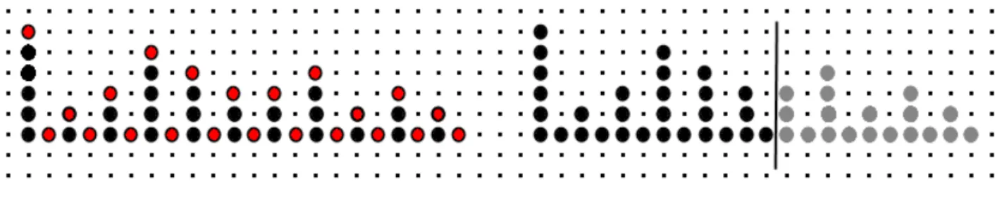
Let us illustrate this with an example. Suppose that we want to dilate a function or a set by an horizontal segment of size 21. Instead of applying 21 successive size 1 dilations, let us perform the following sequence of dilations by a doublet of points: a dilation of size 6, followed on the previous result by a dilation of size 8, followed by a dilation of size 4, then 2 and finally 1. As illustrated in Figure 1, we obtain finally a dilation by a segment of size 21 but with only 5 steps instead of 21. We have potentially multiply by 4 the computation speed.

(a) (b)

Figure 1: (a) successive dilations of an initial point (top line) by doublets of points of respective

sizes 6, 8, 4, 2 and 1. In red, points added at each step. (b) Verification that no edge effect may occur.

How to decompose the initial size n into a suitable sequence as shown before? In fact, when n is equal to 2i_{−1 (i being any positive integer value), the decomposition is straigthforward: the}

successive powers of 2, 2k, with 0 < k < i are used. We can easily see that these dilations produce at

the end a dilation by a segment of size n, provided that we apply these successive dilations in decreasing order (largest one first, size 1 dilation ending necessarily the sequence). When the size is

not equal to but greater than 2i-1, the decomposition is not complicated: we start by substracting 2i_1

from n, 2i-1 being the largest value lower than n. The value n−2i_{1 corresponds to the size of}

the first dilation by a doublet of points. Note that n−2i1 is always lower than or equal to 2i-1.

Then, we decompose the number 2i

-1 as explained above. If the order of operations is respected

(and especially if the first one is the dilation of size n−2i_{1 ), the final transformation is a}

successive operations, you will obtain a segment of size n without holes or missing points. Note also that no edge effects appear: if the initial point is at a distance less then n from the edge, the final result is the intersection of the segment of size n with the field of analysis (Figure 1b).

Compared to the classical implementation, this one is dramatically faster especially when the size n

of the linear structuring element is large. If 2i−1_n2i _{, the speed increase is equal to n/i, that is}

n / int(log2(n)). In fact, this speed gain is lower because the supFarNeighbor operation in Mamba is

a little bit slower than supNeighbor, dilation by an elementary segment. However, for large sizes, this gain is impressive: a dilation by a size 300 segment is about 30 times faster!

Erosions by large segments can be performed in the same way, thanks to the availability of

inFarNeighbor in Mamba. Note also that these transformations can be equally performed in

euclidean or geodesic modes (the edge configuration can be defined in the operators arguments list). These two operators are implemented in largeLinearErode and largeLinearDilate in the Mamba

erodilLarge.py module (see annex). 2.2. Operations with large squares

Performing rapidly erosions and dilations with large squares is straightforward. Indeed, a square belongs to the Steiner class of polygons, which means that erosions and dilations with this structuring element can be decomposed into successive operations with segments. Each segment corresponds to a linear part of its boundary (or more precisely its half-boundary). Therefore, a

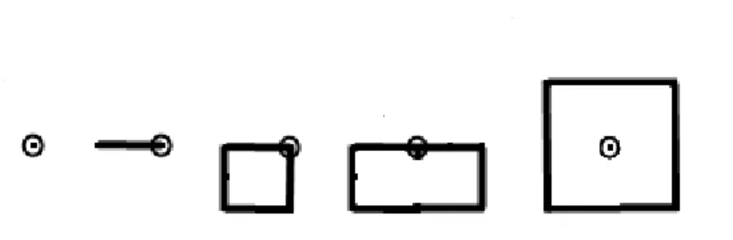
square dilation can be obtained by four successive dilations with segments in the directions 0, π/2, π

and 3π/2 (Figure 2).

Figure 2: Successive dilations of a point by segments in directions 0,

π

π

π

No edge effect is likely to happen for pixels close to the edge because points sent outside the image window by one segment dilation (these points are lost) have no effect on the following dilations which do not need to reinsert them inside the window.

A similar implementation is used for erosions. Theses two operators are named largeSquareErode and largeSquareDilate in erodilLarge.py (see annex).

2.3. Operations with large hexagons

Hexagons belong also to the Steiner class. An hexagonal dilation can be performed (theoretically)

Unfortunately, in practice, this approach does not work properly. The reason? Edge effects... These edge effects have already been encountered when defining the basic hexagonal dilation (size 1 hexagon), see [2]. It is due to the fact that, for pixels near the edge of the image, a dilation in a given direction may propagate a point outside the image window. However, if this dilation is not the last one, the next dilation using another direction should reintroduce inside the image a point resulting of the dilation of the previous pixel, that is not possible because this previous pixel is unfortunately lost (see Figure 3). In order to cope with this problem, the solution, for the elementary hexagon, was to perform a supremum of dilations by segments in the six directions of the hexagonal grid. However, this solution is no longer possible with size n (n > 1) hexagons because it would correspond to dilations by « snowflakes » or asterisks. Thus, we are faced to a dilemma: on the one hand, the Steiner decomposition is compulsory as it is the only way to generate dilations by large hexagons with segments and, on the other hand, we know that this approach leads to unacceptable edge effects.

(a) (b) (c)

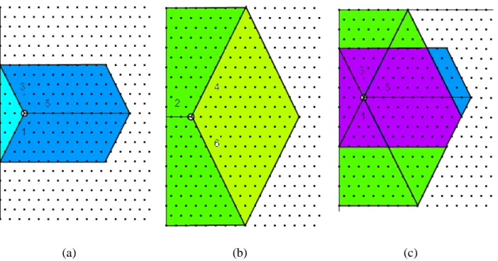
Figure 3: (a) Dilation of a point near the edge by three successive dilations by segments in

directions 1, 3 and 5. (b) Same operation with segments in successive directions 4, 6 and 2. (c) The union of these two results do not prevent edge effects when the initial point is in the upper left corner.

To solve this dilemma, a mixed solution is proposed here, based on suprema of partial dilations obtained by composition of dilations by segments. Indeed, when performing an hexagonal dilation by concatenating linear dilations, different orders are possible: we can use direction 1 first, followed by direction 3 and direction 5. Or we can use another order. Six different orders are available, each one leading to the same result, except if the pixel to be dilated is near an edge. In this case, some orders may produce incorrect results if edge effects appear as illustrated at Figure 3a above.

Therefore, if we perform two dilations, using different directions orders, we may expect that the supremum of these two dilations will produce a result where edge effects have been removed. For instance, if we use successive directions 4, 6 and 2 in the above example, the union of both results produces the awaited hexagonal dilation. In fact, the second dilation alone gives a right result, however using both dilations produces a satisfactory result, the point being near the left or right edges (Figure 3b).

However, we are not sure that this combination will give a correct result whatever the position of the pixel in the image. In fact, in this example, it is not the case. If the pixel to be dilated is near the top left corner of the image, the result is wrong (Figure 3c).

In fact, this approach does not work properly. Whatever the combinations which are used, it is always possible to exhibit counter-examples of pixels which are placed in such a position that edge effects occur.

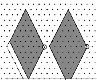
Figure 4: Result of two successive dilations in directions 1 then 3 (left) and in two directions 3

then 1 (right). The first one produces an important edge effect.

Therefore, to be sure to obtain a correct result for all pixels in the image, it is necessary, not only to perform the supremum of partial dilations but also to combine the directions of the linear dilations in such a way that possible edge effects occuring with some combinations of dilations will be compensated by the others. To insure this, the following combination has been used (Figure 4): we perform a dilation by a segment in direction 1 followed by a dilation in direction 3. Then, we perform on the initial image a dilation by a segment in direction 3 followed by a dilation in direction 1. The supremum of these two dilations is computed. Then, the linear dilation of this supremum in direction 5 is performed. Using two dilations in directions 1 and 3 by simply inverting their order allows to remove possible edge effects which could occur when either direction 1 or direction 3 dilation goes over the edge.

Figure 5: First step of the algorithm (left), use of directions 1, 3 and 5. Second step (middle), use

of directions 4, 6 and 2. Note that edge effects do not occur because directions 4 and 6 have been used twice. Supremum of the two previous results (right).

It may happen that both directions produce edge effects (see Figure 5 and examples above). This is why the entire procedure is applied again on the initial image using directions 6, 4 and 2 this time. Finally, the supremum of these two operations is computed to obtain the final result without edge effects.

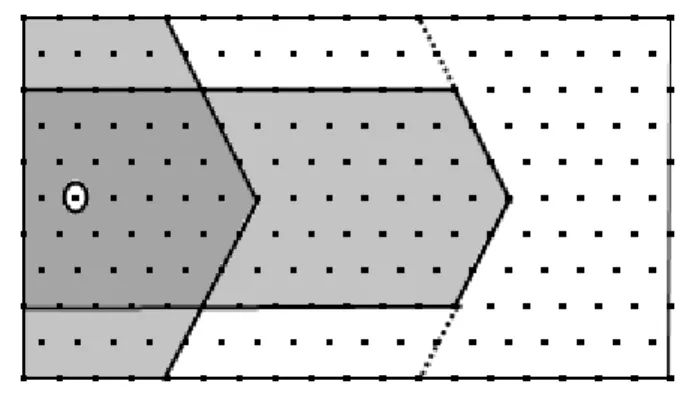
Nevertheless, this procedure assumes that, for at least one direction of linear dilation, the result of this dilation is always contained inside the the image window (Figure 6). If it is not the case, this procedure cannot avoid edge effects leading to a wrong result. This configuration occurs when the hexagon size n is larger then half the window dimensions (width, height). The only solution to avoid this flaw consists in splitting the operation into successive dilations of size i in the following way:

• Perform a dilation of size i = min(width, height)/2 if n > i, of size n if not

• Compute n = (n - i)

• Repeat until n0

Figure 6: When the size of the structuring element is higher than half the size of the window (here,

size is 12 whereas window height is 11), edge effects are unavoidable.

It may seem odd to consider structuring elements larger than the size of the image. However, this situation may happen, when dealing with residual transforms for instance.

The same procedure applies, mutatis mutandis, to large hexagonal erosions.

Both operations are implemented in the erodilLarge.py module. They are named respectively

largeHexagonalErode and largeHexagonalDilate. They work on binary or greytone images. The

edge of the image can be defined in the operations arguments list.

2.4. Operations with large octogons

Large octogons are more interesting than squares on the square grid because they are more isotropic. We already know that an octogonal operation (dilation or erosion) can be achieved by concatenating a square one followed (or preceded) by an operation with a conjugate square or diamond [2]. In order to obtain an isotropic polygon of size n, the respective sizes of the square and diamond operations are given by:

n₁=



n₂=n−n₁= n

1



that is approximately: n₁≃0.41421 n

n₂=n−n1

If the size of images is less than 10000 pixels in height or width, this approximation is sufficient. We already know how to perform rapidly transformations with large squares. Regarding conjugate squares (or diamonds), these structuring elements are also Steiner polygons. However, although

they could be obtained by linear dilations in directions multiples of π/4, this way of doing arises two

problems. The first problem comes from edge effects which have already been described with hexagons. They have the same origin. The second problem is due to the fact that the linear dilations used to generate conjugate squares are defined on the conjugate grid. This leads to dilations with holes as some points are never concerned (Figure 7).

Figure 7: Dilations by segments defined on the conjugate grid. The result is a diamond also

defined on the conjugate grid (hollow diamond).

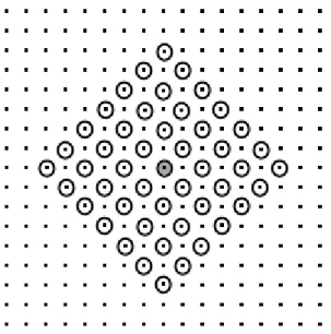
So, to avoid edge effects, an approach based on suprema of dilations by doublets of points is applied to obtain dilations by diamonds. To get a size n diamond, the size is decomposed in the same way as it was done for linear structuring elements. For each value i of the decomposition, a dilation by a "cross" structuring element (Figure 8) is performed.

This structuring element is obtained by the union of dilations by doublets of points in the four horizontal and vertical directions. Dilations are concatenated for all the values of the size decomposition (Figure 8b).

The structuring element generated by this procedure is not a true conjugate square as some holes may appear inside it as shown at Figure 8. Moreover, these holes may sometimes be larger than one pixel wide, especially near the edges. Therefore, this procedure cannot be used to obtain unbiased dilations or erosions by conjugate squares.

Figure 8: "Cross" structuring element of size 4 (left) and result of successive dilations of a point

by this structuring element (sizes 4, 2 and 1) producing a sparse conjugate square of size 7 (right).

But there is an interesting characteristic of this transformation which allows to use it to produce octogonal operations: there is no point missing on the boundary of the structuring element. This can be proved easily when the size n of the structuring element is equal to 2i -1. This size can be decomposed into the successive decreasing values:

2i-1 , 2i-2 , ..., 2 , 1

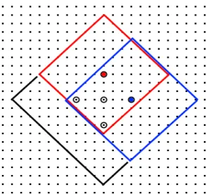
Figure 9: The green pixel on the diamond boundary at coordinates (5, 2) is generated by a size 1

dilation of the red pixel, itself obtained by a size 2 dilation of the blue one. The blue pixel has been generated by a size 4 dilation of the initial yellow center point. These points are always propagated inside the image window (refer to the possible position of an edge indicated by an horizontal line in the figure).

Each point on the boundary is then generated by the dilation by a size 1 "cross" structuring element. The size 1 cross center point is itself generated by a dilation by a size 2 cross and so on (see Figure

9). It is then possible to define a path of horizontal or vertical dilations, all of them inside the image window, from each boundary point towards the initial central point.

More precisely, if the initial central point is at coordinates (0, 0) and the boundary point at

coordinates (x, y) with xy=n=∑ik=0

−1

2k

, it is always possible whatever x and y to write:

x=

∑

k∈I1

2k _{and y=}

∑

k∈I2

2k _{with I}

1≠I2 and I1∪I2={0,i−1}

When n is not equal to but larger than 2i -1, we can perform a first dilation of size n1 = n - 2

i

+ 1

followed by the decomposition of the value 2i

-1 described above. But as n1≤2

i_{−1 , there is}

always an overlap of the boundaries produced by the size 2i

-1 dilations of the cross of size n1

(Figure 10).

Figure 10: Boundary overlapping: the boundaries of the size 7 diamonds generated by the red and

blue pixels overlap, which insures that no boundary point of the final size 10 diamond is missing.

For any size of the dilation, the boundary of the diamond structuring element is complete. So, although it is not possible to obtain a true conjugate square by these means, it is sufficient to get

dilations by octogons. Indeed, we saw that the respective sizes n1 for the square and n2 for the

conjugate square to get an octogonal transformation of size n are given by:

n₁=



1



n

1



So, if we start from an initial point and if we perform first a dilation by a "sparse" diamond of size

n2 as described above, we generate boundary points at a maximum distance n2 from this center point

(indeed, we generate many more points...). Now, if each of these points together with the original

center point are dilated by a square of size n1, all these squares cover the interior of the previous

hollow conjugate square because n1n2 , leading at the end to the generation of an octogon of

size n (Figure 11).

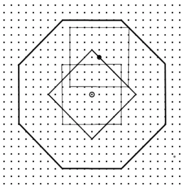
This implementation, both for dilations and erosions, has been realised in largeOctogonalDilate and

Figure 11: Size 10 octogon obtained by a size 6 sparse conjugate square dilation followed by a

size 4 square dilation. We see that the dilations of the center point and of the boundaries of the conjugate square are sufficient to get an octogon without holes.

We may wonder why this approach has not been used with hexagonal structuring elements (that is performing iterations of dilations by a structuring element made of the summits and the center of an hexagon). We let the reader verify that this approach is not very convenient as it produces important edge effects.

2.5. Operations with large dodecagons

We saw previously that performing fast operations with large hexagons was rather tricky if edge effects must be avoided.These edge effects are mainly due to the use of directions non parallel to the edges. They do not appear with squares because only horizontal and vertical directions are used for the dilations or erosions and because no outside point is needed to generate inside ones (each point can be generated by linear dilation from another inside point). We saw also that these dilations by horizontal and vertical doublets of points allow to build hollow conjugate squares which can be used for octogonal operations.

Dodecagonal dilations and erosions being performed by concatenating hexagonal operations and operations by conjugate hexagons, let us describe how faster operations with these latter structuring elements can be achieved.

We explained previously how complex operations with hexagons can be to avoid edge effects. We are faced to the same difficulties with conjugate hexagons. Therefore, the same approach as the one used for conjugate squares has been implemented for conjugate hexagons. This approach generates also sparse or hollow conjugate hexagons. However, these structuring elements are sufficient to perform unbiased dodecagonal erosions and dilations.

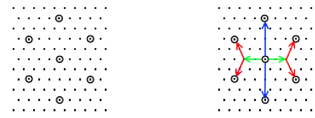
consists in using successive dilations by the following structuring element made of the center and the summits of a conjugate hexagon of size i (Figure 12):

Figure 12: Initial structuring element used to compute sparse conjugate hexagons (left). This

structuring element is obtained by combining shifts (in green) and supFarNeighbor operators (in red) on the hexagonal grid with supFarNeighbor transforms (in blue) on the square grid. Note that the size of this structuring element is 2).

Each size i is obtained by the size decomposition already used above. This structuring element is built by a combination of shifts and of dilations by doublets of points as illustrated at Figure 12. However, edge effects are likely to happen: in directions 1 or 4 first, where the shift operation may push a point outside the image window if the center point is close to the vertical edges. To avoid this bias, one could perform the shift operation twice, in the right and left directions, before computing the corresponding dilation by a doublet. However, this is rather complex and a simple trick allows to cope with this problem. The trick consists in performing a dilation by a doublet of points in the vertical directions 1 or 5 on the square grid!

Edge effects may also appear in other directions as illustrated at Figure 13b. In this case, they come from the proximity of the center point to the horizontal edges. If we consider two successive dilations, the fact that a point has been pushed outside the image window in the first dilation prevents the generation of a necessary point in the following operation (Figure 13c). In order to eliminate this problem, the previous structuring element can be amended by adding two points which correspond to the horizontal summits of the hexagon inscribed in the conjugate hexagon (Figure 13d). So, this point will contribute to the generation of the point which was missing in the previous implementation (Figure 13e). These two points are added by a dilation by doublets of points in directions 3 and 5 (hexagonal grid). If i is the size of the conjugate hexagon (size expressed in number of steps to get it from the elementary conjugate hexagon), the size j of the inscribed hexagon is given by j = 3 i / 2. note that, if i is an odd value, j is given by j=int(3i / 2). In this case, the added point is always inside the conjugate hexagon.

This procedure builds a hollow conjugate hexagon without edge effects thanks to the horizontal and vertical dilations by doublets. Moreover, as for the conjugate square, no point is missing on the boundary (the proof is similar to the one used with conjugate squares). Finally, the respective sizes

n1 and n2 needed for the dilations by an hexagon and a conjugate hexagon to get a size n dodecagon

are given by:

n1=





Now, to cover entirely the conjugate hexagon by dilating its summits and its center by an hexagon in order to fill the holes which remain in it, the minimal size n' of the hexagonal dilation must be

n' = n2. The actual size of the hexagonal dilation is n1=



the covering and the generation of an unbiased dodecagon of size n (Figure 13f).

(a) (b)

(c) (d)

(e) (f)

Figure 13: (a) Concatenation of dilations by the structuring element described above (figure 12).

(b) Edge effects, 2 points are missing. (c) Missed points should have been generated by points which fell outside the image window at the previous step. (d) Modified structuring element, 2 horizontal points are added. (e) Edge effects have been corrected: the previously missing points are generated by the two added points (red points near the edge). (f) Dodecagons obtained by an hexagonal dilation of these sparse conjugate hexagons.

The computation of erosions and dilations by large dodecagons is realised in erodilLarge.py by

largeDodecagonalErode and largeDodecagonalDilate.

3. Performances

The performances of these operators can be coarsely estimated by comparing the number of elementary operations needed to achieve the transformation with the classical approach and with these new implementations.

The transformations with linear structuring elements need the same number of elementary image operators per loop. As this number of loops is lower in the new algorithm than in the classical one, the increase of the computation speed is noticeable from size 2 transform (in fact, it is not exactly the case as the computation time of supFarNeighbor and infFarNeighbor operators is higher than it is with supNeighbor and infNeighbor transforms).

Large square operations are always faster than classical ones because the latter ones do not use the Steiner decomposition of the square contrary to the large ones, so that the number of elementary operations in the first implementation is twice the number of such operators in the second one. If we compare the complexities of the hexagonal classical transformations and of the large hexagonal ones, we can assume that the number of elementary operations to achieve a classical operation of size n is approximately equal to (7 n + 1). The large hexagonal operators are more complex and need a large number of elementary operators per loop. However, this number of loops is given by int(log2(n)+1) when the size of transformation is n. The number of elementary operators

is therefore equal to 10 int(log2(n) + 1) + 14.

The following table indicates the approximate number of operators for hexagonal transforms in the range of sizes [0, 10] and for a size equal to 100. We see that, from size 7, the computation speed for the new implementation overtakes the classical one.

n number of loops (large SE) number of operations (linear ES) number of operations (large lin. SE)

number of operations (hexagon) number of operations (large hexagon) 1 1 2 2 8 24 2 2 3 3 15 34 3 2 4 3 22 34 4 3 5 4 29 44 5 3 6 4 36 44 6 3 7 4 43 44 7 3 8 4 50 44 8 4 9 5 57 54 9 4 10 5 64 54 10 4 11 5 71 54 100 7 101 8 701 84

Figure 14: Respective computation times for classical hexagonal erosions (in blue) and for large

hexagonal ones (in red). The top chart compares binary operations and the bottom one, 8-bits erosions. Times are given in milliseconds. The image size is 768x576 pixels. These tests have been made with a Core 2 Duo 8400 Intel processor, 3 GHz clock, 4 Go RAM memory running on Linux Fedora 13, 64 bits, SSE2 instructions set enabled.

Finally, the curves above (Figure 14) illustrate the speed comparisons between the large hexagonal erosion and the classical hexagonal erosion. We see a dramatic enhancement of the performances obtained by this implementation so that, for size larger than 20, the computation time is almost

independant of the size.

4. Conclusions

We have shown that, from a simple idea (splitting a linear transformation into successive operations by doublets of points), a correct implementation needs an undoubted effort to be efficient and unbiased. But the gain in speed is worth this effort. This complexity explains surely why this approach has been seldom used especially for hardware implementations. It is a matter of fact that a transformation letting edge effects appear is not acceptable.

The implementation which has been achieved in the Mamba library could still be enhanced by coding some operators directly in C instead of Python. However, the present realisation is a compromise between the ease of use and the never ending race to better performances.

5. Acknowledgements

The author wishes to thank Nicolas Beucher for his kind and benevolent help in the achievement of this implementation. Nicolas wrote in particular the C and Python codes for the shift,

supFarNeighbor and infFarNeighbor operators. He also debugged my ackward Python scripts,

tested them and evaluated the performances of this implementation.

6. References

[1] Beucher, Nicolas (2010): Mamba Image Library Python Reference - http://mamba-image.org. [2] Beucher, Serge (2010): Algorithmic description of erosions and dilations in Mamba - To be published by http://mamba-image.org.

[3] Clienti, Christophe (2009): Architectures flot de données dédiées au traitement d'images par Morphologie Mathématique - Doctorat Morphologie mathématique, Centre de Morphologie Mathématique, Mines ParisTech.

[4] Brambor, Jaromír (2006): Algorithmes de la morphologie mathématique pour les architectures orientées flux - Doctorat Morphologie Mathématique, Centre de Morphologie Mathématique, Mines ParisTech..

[5] Sternberg, Stanley (1982): Computer Architectures Specialized for Mathematical Morphology -Workshop on Algorithmically Specialized Computer Organizations, Purdue Univ., West Lafayette, IN, USA..

(Publication date: October 26, 2010)

This document is copyrighted under the Creative Commons "Attribution Non-Commercial No

Annex:

Mamba erodilLarge.py module script

"""

This module provides a set of functions performing erosions and

dilations with large structuring elements. They are built with special shift

operators written in C, together with special 'infFarNeighbor' and 'supFarNeighbor' functions.

"""

# Contributor: Serge BEUCHER, August 1, 2010

import mamba

import mambaComposed as mC

def _sizeSplit(size):

"""

This internal function splits the size of the structuring element into a list of successive and decreasing sizes (except the first one). Successive erosions or dilations by double points produce an erosion or dilation by a segment of length 'size'. """ sizeList=[] incr=1 while size>incr: sizeList.append(incr) size=size-incr incr=2*incr sizeList.append(size) sizeList.reverse() return sizeList

# Elementary operators for large structuring elements

def largeLinearErode(imIn, imOut, dir, size, grid=mamba.DEFAULT_GRID,

edge=mamba.FILLED): """

Erosion by a large segment in direction dir in a reduced number of iterations. Uses the erosions by doublets of points (supposed to be faster, thanks to an enhanced shift operator).

"""

mamba.copy(imIn, imOut) for i in _sizeSplit(size):

mamba.infFarNeighbor(imOut, imOut, dir, i, grid=grid, edge=edge)

def largeLinearDilate(imIn, imOut, dir, size, grid=mamba.DEFAULT_GRID,

edge=mamba.EMPTY): """

Dilation by a large segment in direction dir in a reduced number of iterations. Uses the dilations by doublets of points (supposed to be faster, thanks to

an enhanced shift operator). """

mamba.copy(imIn, imOut) for i in _sizeSplit(size):

mamba.supFarNeighbor(imOut, imOut, dir, i, grid=grid, edge=edge) # Large hexagons

def largeHexagonalErode(imIn, imOut, size, edge=mamba.FILLED):

"""

Erosion by large hexagons using erosions by large segments and the Steiner decomposition property of the hexagon.

Edge effects are corrected by an erosion with transposed decompositions followed by inf operations (see documentation for further details).

This operator is quite complex to avoid edge effects. """

prov1 = mamba.imageMb(imIn) prov2 = mamba.imageMb(imIn) sizemax = min(imIn.getSize())/2

# if size larger than sizemax, the operation must be iterated to prevent edge effects. n = size

mamba.copy(imIn, imOut) while n > 0:

s = min(n, sizemax)

largeLinearErode(imOut, prov1, 6, s, grid=mamba.HEXAGONAL, edge=edge) largeLinearErode(prov1, prov1, 4, s, grid=mamba.HEXAGONAL, edge=edge) largeLinearErode(imOut, prov2, 4, s, grid=mamba.HEXAGONAL, edge=edge) largeLinearErode(prov2, prov2, 6, s, grid=mamba.HEXAGONAL, edge=edge) mamba.logic(prov1, prov2, prov1, "inf")

largeLinearErode(prov1, prov2, 2, s, grid=mamba.HEXAGONAL, edge=edge) largeLinearErode(imOut, prov1, 1, s, grid=mamba.HEXAGONAL, edge=edge) largeLinearErode(prov1, prov1, 3, s, grid=mamba.HEXAGONAL, edge=edge) largeLinearErode(imOut, imOut, 3, s, grid=mamba.HEXAGONAL, edge=edge) largeLinearErode(imOut, imOut, 1, s, grid=mamba.HEXAGONAL, edge=edge) mamba.logic(prov1, imOut, prov1, "inf")

largeLinearErode(prov1, imOut, 5, s, grid=mamba.HEXAGONAL, edge=edge) mamba.logic(imOut, prov2, imOut, "inf")

n = n - s

def largeHexagonalDilate(imIn, imOut, size, edge=mamba.EMPTY):

"""

Dilation by large hexagons using dilations by large segments and the Steiner decomposition property of the hexagon.

Edge effects are corrected by dilations with transposed decompositions followed by sup operators.

This operator is quite complex to avoid edge effects. """

prov1 = mamba.imageMb(imIn) prov2 = mamba.imageMb(imIn) sizemax = min(imIn.getSize())/2

# if size larger than sizemax, the operation must be iterated to prevent edge effects. n = size

mamba.copy(imIn, imOut) while n > 0:

s = min(n, sizemax)

largeLinearDilate(imOut, prov1, 6, s, grid=mamba.HEXAGONAL, edge=edge) largeLinearDilate(prov1, prov1, 4, s, grid=mamba.HEXAGONAL, edge=edge) largeLinearDilate(imOut, prov2, 4, s, grid=mamba.HEXAGONAL, edge=edge) largeLinearDilate(prov2, prov2, 6, s, grid=mamba.HEXAGONAL, edge=edge) mamba.logic(prov1, prov2, prov1, "sup")

largeLinearDilate(prov1, prov2, 2, s, grid=mamba.HEXAGONAL, edge=edge) largeLinearDilate(imOut, prov1, 1, s, grid=mamba.HEXAGONAL, edge=edge) largeLinearDilate(prov1, prov1, 3, s, grid=mamba.HEXAGONAL, edge=edge) largeLinearDilate(imOut, imOut, 3, s, grid=mamba.HEXAGONAL, edge=edge) largeLinearDilate(imOut, imOut, 1, s, grid=mamba.HEXAGONAL, edge=edge) mamba.logic(prov1, imOut, prov1, "sup")

largeLinearDilate(prov1, imOut, 5, s, grid=mamba.HEXAGONAL, edge=edge) mamba.logic(imOut, prov2, imOut, "sup")

n = n - s

# Large squares

def largeSquareErode(imIn, imOut, size, edge=mamba.FILLED):

"""

Erosion by large squares using erosions by large segments and the Steiner decomposition property of the square.

No edge effects are likely to happen with a square structuring element. """

largeLinearErode(imIn, imOut, 1, size, grid=mamba.SQUARE, edge=edge) largeLinearErode(imOut, imOut, 3, size, grid=mamba.SQUARE, edge=edge) largeLinearErode(imOut, imOut, 5, size, grid=mamba.SQUARE, edge=edge) largeLinearErode(imOut, imOut, 7, size, grid=mamba.SQUARE, edge=edge)

def largeSquareDilate(imIn, imOut, size, edge=mamba.EMPTY):

"""

Dilation by large squares using dilations by large segments and the Steiner decomposition property of the square.

No edge effects are likely to happen with a square structuring element. """

largeLinearDilate(imIn, imOut, 1, size, grid=mamba.SQUARE, edge=edge) largeLinearDilate(imOut, imOut, 3, size, grid=mamba.SQUARE, edge=edge) largeLinearDilate(imOut, imOut, 5, size, grid=mamba.SQUARE, edge=edge) largeLinearDilate(imOut, imOut, 7, size, grid=mamba.SQUARE, edge=edge)

# Large dodecagons

def _sparseConjugateHexagonErode(imIn, imOut, size, edge=mamba.FILLED):

"""

Erosion by a conjugate hexagon. The structuring element used by this operation is not complete. Some holes appear inside the structuring element. Therefore, this operation should not be used to obtain true conjugate hexagons dilations (for internal use only).

""" prov1 = mamba.imageMb(imIn) prov2 = mamba.imageMb(imIn) mamba.copy(imIn, imOut) val = mamba.computeMaxRange(imIn)[1]*int(edge==mamba.FILLED) for i in _sizeSplit(size): mamba.copy(imOut, prov1) j = 2*i

mamba.infFarNeighbor(prov1, imOut, 1, j, grid=mamba.SQUARE, edge=edge) mamba.shift(prov1, prov2, 2, i, val, grid=mamba.HEXAGONAL)

mamba.infFarNeighbor(prov2, imOut, 4, i, grid=mamba.HEXAGONAL, edge=edge) mamba.infFarNeighbor(prov2, imOut, 6, i, grid=mamba.HEXAGONAL, edge=edge) mamba.infFarNeighbor(prov1, imOut, 5, j, grid=mamba.SQUARE, edge=edge) mamba.shift(prov1, prov2, 5, i, val, grid=mamba.HEXAGONAL)

mamba.infFarNeighbor(prov2, imOut, 1, i, grid=mamba.HEXAGONAL, edge=edge) mamba.infFarNeighbor(prov2, imOut, 3, i, grid=mamba.HEXAGONAL, edge=edge) j = 3*i/2

mamba.infFarNeighbor(prov1, imOut, 2, j, grid=mamba.HEXAGONAL, edge=edge) mamba.infFarNeighbor(prov1, imOut, 5, j, grid=mamba.HEXAGONAL, edge=edge)

def _sparseConjugateHexagonDilate(imIn, imOut, size, edge=mamba.EMPTY):

"""

Dilation by a conjugate hexagon. The structuring element used by this operation is not complete. Some holes appear inside the structuring element. Therefore, this operation should not be used to obtain true conjugate hexagons dilations (for internal use only).

""" prov1 = mamba.imageMb(imIn) prov2 = mamba.imageMb(imIn) mamba.copy(imIn, imOut) val = mamba.computeMaxRange(imIn)[1]*int(edge!=mamba.EMPTY) for i in _sizeSplit(size): mamba.copy(imOut, prov1) j = 2*i

mamba.supFarNeighbor(prov1, imOut, 1, j, grid=mamba.SQUARE, edge=edge) mamba.shift(prov1, prov2, 2, i, val, grid=mamba.HEXAGONAL)

mamba.supFarNeighbor(prov2, imOut, 4, i, grid=mamba.HEXAGONAL, edge=edge) mamba.supFarNeighbor(prov2, imOut, 6, i, grid=mamba.HEXAGONAL, edge=edge) mamba.supFarNeighbor(prov1, imOut, 5, j, grid=mamba.SQUARE, edge=edge) mamba.shift(prov1, prov2, 5, i, val, grid=mamba.HEXAGONAL)

mamba.supFarNeighbor(prov2, imOut, 1, i, grid=mamba.HEXAGONAL, edge=edge) mamba.supFarNeighbor(prov2, imOut, 3, i, grid=mamba.HEXAGONAL, edge=edge) j = 3*i/2

mamba.supFarNeighbor(prov1, imOut, 2, j, grid=mamba.HEXAGONAL, edge=edge) mamba.supFarNeighbor(prov1, imOut, 5, j, grid=mamba.HEXAGONAL, edge=edge)

def largeDodecagonalErode(imIn, imOut, size, edge=mamba.FILLED):

"""

Erosion by large dodecacagons (hexagonal grid). Basically, it is the same operation as the previous one where classical erosions have been replaced by erosions by large structuring elements, and where a "partial" erosion by a conjugate hexagon is used.

"""

n1 = int(0.4641*size)

n1 += abs(n1 % 2 - size % 2) n2 =(size - n1)/2

_sparseConjugateHexagonErode(imIn, imOut, n2, edge=edge) largeHexagonalErode(imOut, imOut, n1, edge=edge)

def largeDodecagonalDilate(imIn, imOut, size, edge=mamba.EMPTY):

"""

Dilation by large dodecacagons (hexagonal grid). Basically, it is the same operation as the previous one where classical dilations have been replaced by dilations by large structuring elements, and where a "partial" dilation by a conjugate hexagon is used.

"""

n1 = int(0.4641*size)

n1 += abs(n1 % 2 - size % 2) n2 =(size - n1)/2

_sparseConjugateHexagonDilate(imIn, imOut, n2, edge=edge) largeHexagonalDilate(imOut, imOut, n1, edge=edge)

def _sparseDiamondDilate(imIn, imOut, size, edge=mamba.EMPTY):

"""

Dilation by a large diamond (losange) on square grid. This diamond is not completely filled. It is for internal use only.

"""

prov = mamba.imageMb(imIn) mamba.copy(imIn, imOut) for i in _sizeSplit(size): mamba.copy(imOut, prov)

mamba.supFarNeighbor(prov, imOut, 1, i, grid=mamba.SQUARE, edge=edge) mamba.supFarNeighbor(prov, imOut, 3, i, grid=mamba.SQUARE, edge=edge) mamba.supFarNeighbor(prov, imOut, 5, i, grid=mamba.SQUARE, edge=edge) mamba.supFarNeighbor(prov, imOut, 7, i, grid=mamba.SQUARE, edge=edge)

"""

Erosion by a large diamond (losange) on square grid. This diamond is not completely filled. It is for internal use only.

"""

prov = mamba.imageMb(imIn) mamba.copy(imIn, imOut) for i in _sizeSplit(size): mamba.copy(imOut, prov)

mamba.infFarNeighbor(prov, imOut, 1, i, grid=mamba.SQUARE, edge=edge) mamba.infFarNeighbor(prov, imOut, 3, i, grid=mamba.SQUARE, edge=edge) mamba.infFarNeighbor(prov, imOut, 5, i, grid=mamba.SQUARE, edge=edge) mamba.infFarNeighbor(prov, imOut, 7, i, grid=mamba.SQUARE, edge=edge)

def largeOctogonalErode(imIn, imOut, size, edge=mamba.FILLED):

"""

Erosion by a large octogon (square grid). This operation uses erosions by large squares and large diamonds previously defined.

"""

n1 = int(0.41421*size + 0.5) n2 = size - n1

largeSquareErode(imIn, imOut, n1, edge=edge) _sparseDiamondErode(imOut, imOut, n2, edge=edge)

def largeOctogonalDilate(imIn, imOut, size, edge=mamba.EMPTY):

"""

Dilation by a large octogon (square grid). This operation uses dilations by large squares and large diamonds previously defined.

"""

n1 = int(0.41421*size + 0.5) n2 = size - n1

largeSquareDilate(imIn, imOut, n1, edge=edge) _sparseDiamondDilate(imOut, imOut, n2, edge=edge)