HAL Id: hal-00722633
https://hal-mines-paristech.archives-ouvertes.fr/hal-00722633
Submitted on 2 Aug 2012
HAL is a multi-disciplinary open access
archive for the deposit and dissemination of
sci-entific research documents, whether they are
pub-lished or not. The documents may come from
teaching and research institutions in France or
abroad, or from public or private research centers.
L’archive ouverte pluridisciplinaire HAL, est
destinée au dépôt et à la diffusion de documents
scientifiques de niveau recherche, publiés ou non,
émanant des établissements d’enseignement et de
recherche français ou étrangers, des laboratoires
publics ou privés.
Multi-scale statistical approach of the elastic and
thermal behavior of a thermoplastic polyamid glass fiber
composite
Mamane Oumarou, Dominique Jeulin, Jacques Renard, Philippe Castaing
To cite this version:
Mamane Oumarou, Dominique Jeulin, Jacques Renard, Philippe Castaing. Multi-scale statistical
ap-proach of the elastic and thermal behavior of a thermoplastic polyamid glass fiber composite.
Technis-che Mechanik, Magdeburger Verein für TechnisTechnis-che Mechanik e.V., 2012, 32, pp.484-506. �hal-00722633�
TECHNISCHE MECHANIK,
32, 2-5, (2012), 484 - 506 Submitted: November 1, 2011Multi-Scale Statistical Approach of the Elastic and Thermal
Behavior of a Thermoplastic Polyamid-Glass Fiber Composite
M. M. Oumarou, D. Jeulin, J. Renard, P. Castaing
The strong heterogeneity and the anisotropy of composite materials require a rigorous and precise analysis as a result of their impact on local properties. First, mechanical tests are performed to determine the macroscopical behavior of a polyamid glass fiber composite. Then we focus on the influence of the heterogeneities of the microstructure on thermal and mechanical properties from finite element calculations on the real microstructure, after plane strain assumptions. 100 images in 10 different sizes (50, 100, 150, 200, 250, 300, 350, 400, 450, 600 pixels) are analysed. The influence of the area fraction and the spatial arrangement of fibers is then established. For the thermal conductivity and the bulk modulus the fiber area fraction is the most important factor. These properties are improved by increasing the area fraction.
On the other hand, for the shear modulus, the fibers spatial arrangement plays the paramount role if the size of the microstructure is smaller than the RVE. Therefore, to make a good prediction from a multi-scale approach the knowledge of the RVE is fundamental.
By a statistical approach and a numerical homogenization method, we determine the RVE of the composite for the elastic behavior (shear and bulk moduli), the thermal behavior (thermal conductivity), and for the area fraction. There is a relatively good agreement between the effective properties of this RVE and the experimental macroscopical behavior. These effective properties are estimated by the Hashin-Shtrikman lower bound.
1 Introduction
This work is carried out on a composite with a thermoplastic matrix reinforced by continuous glass fibers. Tests at macroscopical scale give relatively homogeneous results with a reduced standard deviation. However, the microstructure analysis of the same samples shows several heterogeneities related to the manufacturing process of the material and the geometry of their components. The study of the microstructure of heterogeneous materials became an important branch of research during the five last decades (Hill, 1963; Hashin and Shtrikman, 1963; Matheron, 1971; Willis, 1981; Serra, 1982; Jeulin, 1991; Drugan and Willis, 1996). To have a better prediction of these materials, different scales have to be considered: microscopical scale (size of fibers), mesoscopical scale (intermediate size) and macroscopical scale (size of samples). This is commonly called a multi-scale approach (Jeulin, 1991; Jeulin and Ostoja-Starzewski, 2001).
The aim of this approach is to determine the smallest volume which allows for a good estimation of the macroscopical properties of the material, and which will be large enough to take into account all heterogeneities at a microscopical scale. It is the Representative Volume Element (RVE) (Sun and Vaidya, 1996; Andrei, 1997; Ostoja-Starzewski, 2002; Shan and Gokhale, 2002; Kanit et al., 2003; Xiangdong and Ostoja-Starzewski, 2006; Ostoja-Starzewski, 2006; Trias et al., 2006; Gitman et al., 2007; Grufman and Ellyin, 2007; Zeman and Sejnoha, 2007; Thomas et al., 2008; Frank Xu and Chen, 2009).
The RVE became a scientific concept with many interpretations according to various authors. Some authors choose the geometrical criteria of the components (Willis, 1981; Ostoja-Starzewski, 1993, 1998, 2002, 2006, 2007; Jiang et al., 2001).
Moreover, it is shown that the RVE is related to the ratio of the size of the microstructure on the diameter of fibers. This ratio equals 50 (Trias et al., 2006). Others showed the influence of the contour of the microstructures, as well as the volume fraction of the clusters (Bhattacharyya and Lagoudas, 2000; Jiang et al., 2001; Segurado and LIorca, 2006; Jan et al., 2006). In other works, the RVE is determined according to the fibers spatial arrangement and the distance between fibers (Jiang et al., 2001; Knight et al., 2003).
Thomas et al. (2008), following Kanit et al. (2003), fixed a relative error and the smallest RVE is the first size for which the precision reaches this value. On the other hand, they stipulate that the RVE is reached only when (the standard deviation) is minimum and tends to a rather constant value. They applied this approach to the fiber area fraction and the thermal conductivity of a carbon-epoxy composite.
In our case, the RVE cannot only depend on the size of fibers and microstructure. The diameter of fibers varies much with a coefficient of variation of approximately 13%. When we consider only one size of the diameter, we move away from the real microstructure of the studied composite.
In addition, in Trias et al. (2006), it is stipulated that the inhomogeneities in the particle spatial distribution had a negligible influence on the effective properties of the composite in the elastic and plastic regimes. This is true, in our case, only if the volume is larger than the smallest RVE.
On the contrary, there is a property (shear modulus), for which this inhomogeneity (spatial arrangement) can play a more important role than the area fraction.
To determine a statistical RVE objectively, Kanit et al. (2003) have developed the use of statistical tools able to take into account all these dispersions (area fraction, size of fibers, contour, fibers spatial arrangement, size of microstructures, precision, standard deviation, etc). We adopt this method to determine the RVE for the area fraction, the thermal conductivity, and the elastic behavior of the composite. This RVE depends on the measured property. The final RVE will be the largest of all RVEs. It will be shown that it is equal to 854´854mm (for
100 =
N images), and contains 1310 fibers in average.
The effective properties of this RVE are compared to the macroscopical behavior of the composite. These properties can be locally estimated by Hashin-Shtrikman lower bounds.
2 Macroscopic Approach 2.1 Material and Method
The material is a composite made of a polyamid matrix (PA6) and continuous glass fibers reinforcement (Figure1-a). Its fabrication is based on a homogeneous mixture of fibers and matrix. This innovative product brings several advantages such as the recyclability, the weldability, a good impregnation of glass fibers by the resin, and the absence of volatile organic compounds.
In the macroscopical approach, the mechanical behavior (bulk and shear moduli) and the volume fraction of the composite are studied.
a) b)
Figure 1. a) Plate of composite (300mm´300mm´2.4mm); b) Samples for mechanical tests
2.1.1 Mechanical Behaviour
Plates of a unidirectional composite are provided by CETIM (Centre Technique des Industries Mécaniques), Figure 1-a.
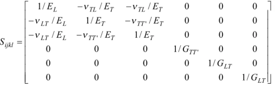
A unidirectional composite (with long fibers reinforcement) is characterized by a transversely isotropic behavior (Berthelot, 1999; Bunsel and Renard, 2005) which is defined by the knowledge of 5 coefficients in the elastic regime:
(
EL,ET,GLT,nLT,nTT')
, where E is the longitudinal modulus, L E the transverse modulus, T GLT thelongitudinal shear modulus, nLTthe longitudinal Poisson’s ratio and nTT' the transverse Poisson’s ratio. These coefficients are obtained by the generalized Hooke’s law, in which a linear relation is established between the strain and the stress fields,
kl ijkl ij kl ijkl ij C e or e S s s = = (1)
Where Cijkl is the stiffness matrix and Sijkl the complience matrix.
Samples of dimensions 200mm 25´ mm are cut, Figure 1-b. This size is so large that all local dispersions are removed. Standards into epoxy with 60mm of length are stuck to the edges of the samples (Figure 1-b) to avoid
damage starting there, as a result of the clamping force. The working length is 80mm, sufficient to place extensometers, and to satisfy the principle of Saint Venant.
The moduli are determined by quasi static tensile tests carried out on an Instron’s dynamometer, equipped with a loading cell of 100kN. Displacement control is used. Two extensometers record longitudinal and transverse displacement, and enable us to determine the Poisson’s ratios.
These tensile tests are performed in the direction parallel to fibers (for E and L nLT
)
, perpendicular to fibers (forT
E , and nTT'
)
, and in 45° compared to the direction of fibers (for GLT)
(Figure 1-b).The stiffness matrix is determined by reversing the complience matrix given bellow
ú
ú
ú
ú
ú
ú
ú
ú
û
ù
ê
ê
ê
ê
ê
ê
ê
ê
ë
é
-=
LT LT TT T T TT L LT T TT T L LT T TL T TL L ijklG
G
G
E
E
E
E
E
E
E
E
E
S
/
1
0
0
0
0
0
0
/
1
0
0
0
0
0
0
/
1
0
0
0
0
0
0
/
1
/
/
0
0
0
/
/
1
/
0
0
0
/
/
/
1
' ' 'n
n
n
n
n
n
(2)The other coefficients (nTL,GTT') of the stiffness matrix are determined by the relations due to the symmetries of the transversly isotropic behavior, as given in equaitons bellow
L T LT TL E E n n = (3)
(
')
' 21 TT T TT E G n + = (4) 2.1.2 Volume FractionSamples of dimensions 20mm 50´ mm are cut out in the plates and weighed. Then they are placed in an oven at
C
°
500 during 1 hour for pyrolysis, to determine the mass fraction of the fibers (Figure 2). This enables us to determine the macroscopical fibers volume fraction.
Figure 2. Glass fibers after pyrolysis
2.2 Experimental Results 2.2.1 Mechanical Behavior
After tensile tests, the mechanical macroscopic behavior is given in Table 1. Then we obtain the stiffness matrix of the composite.
Table 1. Experimental result
L
E E T GLT nLT nTT'
GPa
C
macroú
ú
ú
ú
ú
ú
ú
ú
û
ù
ê
ê
ê
ê
ê
ê
ê
ê
ë
é
=
66
.
1
0
0
0
0
0
0
66
.
1
0
0
0
0
0
0
1
.
2
0
0
0
0
0
0
00
.
9
81
.
4
84
.
4
0
0
0
81
.
4
00
.
9
84
.
4
0
0
0
84
.
4
84
.
4
39
.
38
For simplifications, we consider the bulk modulus (K=(C22+C23)/2) and the transverse shear modulus (m=GTT'), which can represent this elastic behavior, and which are given by: Kmacro=6.90GPa and
GPa
macro23 =2.1
m .
2.2.2 Volume Fraction
After pyrolysis, the density of the composite is determined (1.616 g.cm- 3). The rate of porosity (which is the
ratio between the theorical and measured density) is of 0.27%. The fibers mass fraction (Figure 2) is determined as 59%. Thus, the macroscopical fibers volume fraction is 40%.
3 Microscopic Approach
In this approach, the composite is not regarded as one indissociable material. It is rather regarded as a field made up of separable physical entities: fibers and matrix, and, possibly, inclusions and defects in the matrix (voids). In this procedure, only the fibers and the matrix are taken into account.
The purpose of this section is to determine from a multiscale approach the RVE of studied properties (area fraction, thermal conductivity, elastic moduli) according to the relative error, by using morphological and statistical tools. Then by a numerical homogenization the effective properties of this RVE will be determined and compared to the macroscopical behavior characterized above.
First, an image analysis is performed to characterize the microstructure of the composite using the software MICROMORPH, developed by Centre de Morphologie mathématique of Ecole des Mines de Paris. The analysed images are from SEM (Scanning Electron Microscop) after polishing.
3.1 Image Analysis
The characterization of a random medium is based on morphological measuring criteria. These criteria are based on the stereology (surface and volume fraction measurement) size distribution (2D, 3D), distribution in space (clusters, anisotropy, etc) and connectivity. The principle of this measurement is based on two steps: morphological transformation applied to the microstructure, and measurement of objects contained in the transformed microstructure (Serra, 1982).
The realization of these steps requires well adapted morphological tools which take into account all dispersions (local dispersions (area fraction, size of fibers), and fibers spatial arrangement). These dispersions must be taken into account in the determination of the RVE. Consequently it is not exact to consider a unit cell as representative volume element for this type of material.
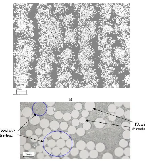
The microstructures resulting from the SEM are on grey level (luminosity between 0 and 255, Figure 3-a-b) with a depth of 8 bits per pixel. The first transformation consists of making them binary (Figure 4-a).
a)
b)
Figure 3. a) Fibers spatial arrangement (scale = 200mm); b) Local fluctuations of microstructures
a) b)
Figure 4. Image segmentation
The separation of fibers was made by an image segmentation procedure, so that the detected fibers remain surrounded by the matrix in the further steps of the calculations (Figure 4-b).
These stages enable one to apply the morphological tools such as the covariance and the integral range which are briefly described bellow.
3.1.1 The Covariance
The covariance provides several information of the microstructure, such as the spatial distribution of the components and their size, the anisotropy (or not), the periodicity and the volume fraction (area fraction in 2 D). Morphologically it is defined for a subset Kmade up of the couple of points
{ }
x and{
x+ by the probability h}
(
x x h) {
P x A x h A}
C , + = Î , + Î (5)
3.1.2 The Integral Range
The integral range is a very important concept for the statistical processing of the heterogeneous microstructures (Matheron, 1971; Serra, 1982; Jeulin, 1991; Kanit et al., 2003). For a given microstructure, it determines a domaine size for which the parameters measured in this volume have a good statistical representativity.
In a space R , it can be written as n
( ) ( )
-ò
(
( ) ( )
-)
= n R n Ch C dh C C A 2 02 0 0 1 (6) Where A is the integral range and n C(h) the covariance.For a volume V ( S in 2 D), the variance of an average property Z in V can be expressed according to the integral range and the local variance
if V >> An then
( )
V A D V D n Z Z2 = 2 (7) 2 ZD being the local variance.
3.2 Determination of the RVE
As seen previously, there are many definitions for the RVE of heterogeneous materials. The most important ones are:
Definition 1: The RVE is (a) a sample that is structuraly entirely typical of the whole mixture on average, and (b) contains sufficient number of inclusions for the apparent overal moduli to be effectively independent of the surface values of traction and displacement, so long as these values are macroscopically uniform (Hill, 1963). Definition 2: The RVE is the smallest material volume element of the composite for which the usual spatially constant overal modulus macoscopic constitutive representation is a sufficiently accurate model to represent mean constitutive response (Drugan and Willis, 1996).
The RVE defines the mesoscopical scale (Hill, 1963; Drugan and Willis, 1996; Jiang et al., 2001; Kanit et al., 2003; Ostoja-Starzewski, 2002, 2006; Trias et al., 2006). To be practical and applicable, the Definition 1 requires the use of statistical tools on microstructures. And it enables one to obtain the evolution of the RVE according to the relative statistical error resulting from fluctuations of the microstructure and of the fields (Kanit et al., 2003). In fact the accuracy of the estimation of the average property Z of a random variable is given by the absolute error
( )
n S DZ abs= 2 e (8)The relative error is then deduced
( )
n Z S D Z Z abs rel 2 = =e e (9)The variance of the random variable Z can be written according to the local variance and the integral range, for very large area S (Matheron, 1971; Serra, 1982; Kanit et al., 2003):
( )
S A D S DZ2 = Z2 2 (10)By replacing the variance by its value in equation (10), the evolution of the statistical RVE is obtained according to the integral range, the average value Z, the number of observations (images of the microstructure), and the chosen relative error
2 2 2 2 4 Z n A D V r Z ER= e (11)
In practice, we can work with a single large image (using n=1 in equation (11)), or use n smaller images with an area equal to the RVE. In what follows we will take n=100.
The Definition 2 provides the average of the fields of the measured properties (homogenization), and makes it possible to choose that particular RVE which will be the smallest of RVEs which does not depend on boundary conditions (Hill, 1963; Kanit et al., 2003). Both methods appear complementary rather than opposing. Still, the elementary surface S of images in equation (10) should be larger than the smallest size of the microstructure, in order to insure that no bias is generated by boundary conditions in the estimation of the effective properties. Moreover, a heterogeneous material has a RVE for each property, and the final RVE will be the larger one.
3.3 Homogenization
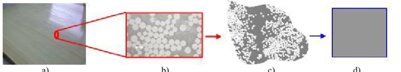
The homogenization of a heterogeneous medium (Figure 5) consists of determining the equivalent homogeneous medium (EHM), after removing the local fluctuations, (Hill, 1963; Willis, 1981; Torquato, 1991; Lukkassen et al, 1995; Nemat-Nasser and Hori, 1999; Jeulin and Ostoja-Starzewski, 2001).
a) b) c) d)
Figure 5. Homogenization process. a) macroscopical scale; b) microscopical scale; c) mesoscopical scale; d) EHM
In the next subsections, finite element method (FEM) homogenization is studied and compared by the bounds estimation. The influence of the boundary conditions on the measured properties is highlighted.
3.3.1 FEM Homogenization
The development of new softwares and reliable tools for microstructures analysis makes the homogenization by the finite element method (FEM) possible. By integrating all heterogeneities, the FEM is very efficient to estimate the effective properties. The meshing process is carried out with the software AVIZO, while Zebulon (developed by Ecole des Mines de Paris and ONERA) is used for finite element calculations.
Figure 6. Image preparing and meshing process
The plane strain assumption enables one to work in the plane perpendicular to the cross section of the fibers. The C2d3 type of element is used.
For each property 100 images of the microstructure are considered for 10 different sizes. Specific boundary conditions are needed to determine the effective properties of the composite (see the subsections bellow). The effective value is reached when the measured property does not depend on the type of boundary conditions any more.
The physical properties which will be studied by the FEM are given in Table 2.
a) FEM homogenization of the thermal conductivity
In this part, a thermal steady state problem is studied, by imposing a uniform temperature gradient on the contours of images of the microstructures (see equation (12)). The thermal conductivity is determined by studying the heat flux of the composite using Fourier’s law (see equation (13)).
V x x G T = " ζ (12) T qij=-lijÑ (13)
Where q is the heat flux, TÑ the temperature gradient, and
l
the thermal conductivity tensor. The average heat flux is obtained by averaging the local fields in the microstructure.ò
=VqdV
V
Q 1 (14)
To highlight the influence of the anisotropy of the microstructure on the thermal behavior, the gradient of temperature is imposed in two directions (horizontal and vertical).
b) FEM homogenization of the elastic properties
For the mechanical problem, we will study the bulk modulus and the transverse shear modulus of images by assuming an isotropic elastic behavior of the fibers and of the matrix.
Table 2. Physical properties to be studied
Problem Flux Measured field Measured properties
Heat conduction Heat flux Temperature gradient Thermal conductivity
On each image, kinematic uniform boundary conditions called KUBC are imposed (see equation (15)). These conditions result in a uniform displacement of all points of the contour
V ~ " ζ
=Ex x
u (15)
Thus, it is possible to determine the average stress in the microstructure by averaging the local stress fields (see equation 16) dV V
ò
V = = S ~ ~ ~ 1 s s (16)It should be noted that there exist other boundary conditions such as SUBC (Static Uniform Boundary Conditions which lead to uniform stress conditions on the contours) and the periodic boundary conditions. However it is shown in several works that KUBC and SUBC conditions are two different ways to obtain asymptotically the same result, provided the images are large enough and thus statistically representative (Jeulin and Ostoja-Starzewski, 2001; Jiang et al., 2002; Kanit et al., 2003; Trias et al., 2006; Zeman and Sejnoha, 2007).
3.3.2 Bounds Method Homogenization
The variational bounds and estimations have been used to determine homogenized properties of a random medium for several decades (Willis, 1981; Nemat-Nasser and Hori, 1999; Jeulin and Ostoja-Starzewski, 2001; Ostoja-Starzewski, 1998, 2007). Some of them are more accurate than others. For example, the first order bounds of Voigt and Reuss (Swan and Kosaka, 1997) only take into account the volume fraction of the components. The Hashin-Shtrikman second order bounds take into account the volume fraction and the isotropy of the microstructure (Willis, 1981; Berthelot, 1999; Kanit et al, 2003). In addition, the estimations of Mori Tanaka take into account the spherical particles in an isotropic elastic matrix (Mori and Tanaka, 1973).
In this work, only Hashin-Shtrikman bounds are studied.
For a transversely isotropic composite with random arrangement of fibers, the 2D Hashin-Shtrikman upper and lower bounds for shear modulus (see equation (17) and (18)), and bulk modulus (see equation (19) and (20)) are given by (Berthelot, 1999)
(
f f)
f f f v f m v f H K K F F m m m m m m m + + + -+ = + 2 2 1 1 23 (17)(
)
(
)
m m m m m v m f v m H K K F F m m m m m m m + + -+ -+ = -2 2 1 1 23 (18)(
f f)
v f m v f H K F K K F K K m + + -+ = + 1 1 (19)(
m m)
v m f v m H K F K K F K K m + -+ -+ = -1 1 (20) where K(
E)
(
E)
i m f i i i i ii=31-2n m =21+n = , for matrix and fiber, F is the volume fraction v
For the thermal conductivy, the upper and lower bounds of Hashin-Shtrikman in 2D are given by
f f V f m m V f HS F F l l l l l 2 1 + -+ = + (21)
m m V m f f V m HS F F l l l l l 2 1 + -+ = -(22)
where
l
f andl
m are (respectively) the thermal conductivity of fibers and matrix.3. 4 Numerical Simulation and Image Analysis Results 3.4.1 Fibers Spatial Arrangement
For a stationary random set as will be assumed here, the covariance does not depend on the point x .
By taking h=0 in equation 3, one reaches the area fraction (equivalent to the volume fraction) of fibers, 40% (Figure 7-c).
The changing of the covariance according to the direction (horizontal or vertical) shows the anisotropy of the microstructure on scale of ply (Figure 7-a, and 7-b), and highlights its periodicity in the horizontal direction (Figure 7-a and 7-c).
0 500 1000 1500 2000 2500 3000 3500 4000 4500 5000 0 100 200 300 400 500 600 700 800 Distance (um) a) 0 500 1000 1500 2000 2500 3000 3500 4000 4500 5000 0 100 200 300 400 500 600 700 800 Distance (um) b) c)
Figure 7. a) Horizontal covariance; b) Vertical covariance; c) Horizontal average covariance (for 100 microstructures)
Three inflexions appear on the covariance curve (Figure 7-c). The x coordinate of the first inflexion point indicates the average value of the diameter of the fibers (16mm). Similarly the average size of plys (232mm), and the average distance between centers of plys (439mm) and thus the average size of the poor zone of the fibers (207mm) are obtained.
3.4.2 Fluctuations of Fibers Area Fraction
To determine the area fraction by image analysis, 100 images of different sizes
(50´50,100´100,150´150,200´200,250´250,300´300,350´350,400´400,450´450,600´600 pixels) are randomly taken in the microstructure.
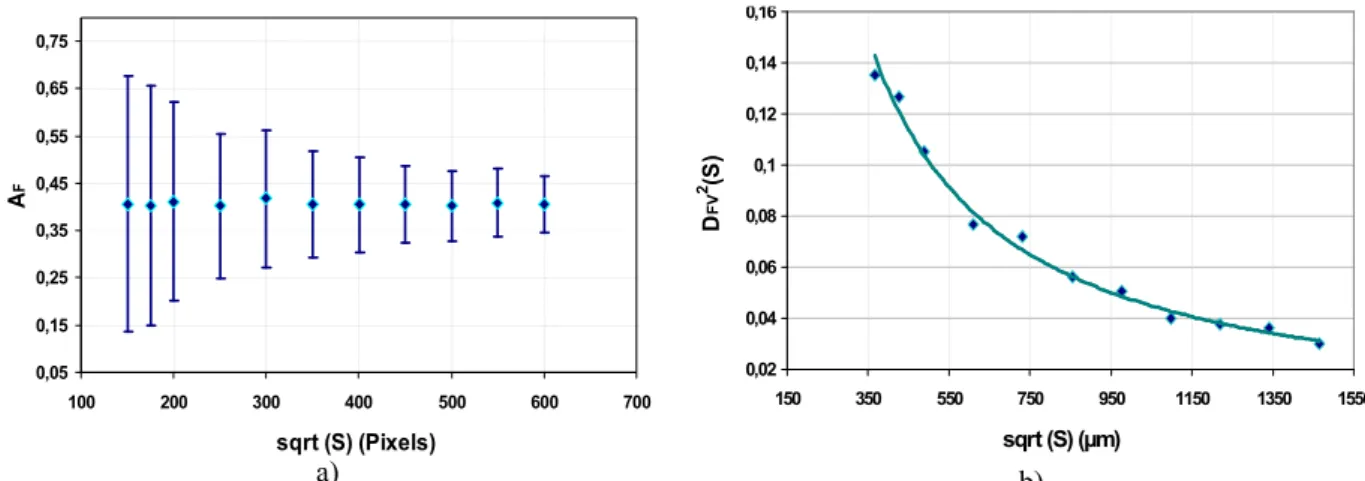
It can be observed that the area fraction does not depend on the size of the studied image (Figure 8-a), and that the variance and the interval of confidence decrease when the size of the image increases (Figure 8-b), (Drugan and Willis, 1996; Kanit et al., 2003). The average area fraction is 40% (Figure 8-a).
0,05 0,15 0,25 0,35 0,45 0,55 0,65 0,75 100 200 300 400 500 600 700 sqrt (S) (Pixels) A F a) 0,02 0,04 0,06 0,08 0,1 0,12 0,14 0,16 150 350 550 750 950 1150 1350 1550 sqrt (S) (µm) D FV 2(S) b)
Figure 8. a) Area fraction according to the image size; b) Variance of the area fraction
3.4.3 Fibers Size Fluctuations
To analyse the dispersions of the size of the fibers, three images of 600´600 pixels (1464´1464mm2) were randomly taken. Each one of these images contains more than 3000 fibers. This makes a total of more than 11.000 fibers to be analyzed. The results are given in Table 3.
3.4.4 Influence of Fibers Spatial Arrangement on the Local Thermal Conductivity
For the calculations, the input thermal conductivities of the fibers and of the matrix are respectively 1.W
( )
mK -1and 0.2W
( )
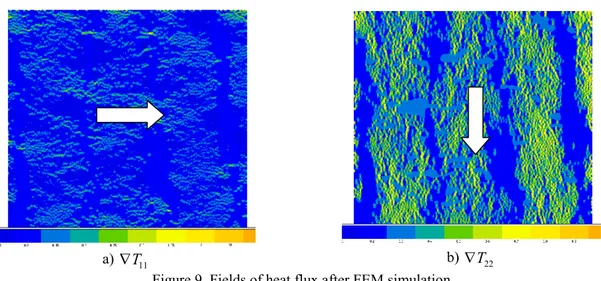
mK -1.The FEM calculations provide the fields of the heat flux (Figure 9). We thus determine the thermal conductivity of the composite in two directions (orthogonal and parallel to the beams of fibers) for images of different sizes. Table 3. Size of fibers and dispersions (for 11237 fibers)
Average Standard
deviation
f
minf
max Coefficient of variation confidence at 95% Interval of average diameter ofa)
Ñ
T
11 b) ÑT22Figure 9. Fields of heat flux after FEM simulation
If the temperature gradient is applied orthogonally to the beams of fibers, the thermal conductivity is lower. However, it remains quasi homogeneous in the microstructure (Figure 9-a). It is higher in the case of a gradient parallel to the beams, with the risk of local overheating in zones with strong density of fiber (Figure 9-b). A relationship between the local area fraction and the thermal conductivity of 100 different images of the microstructures from different sizes is examined. It can be observed in both cases that the thermal conductivity depends mainly on the temperature gradient and especially the fiber area fraction. This is shown by the quasi linear relation in Figure 10-a and 10-b.
0 0,1 0,2 0,3 0,4 0,5 0,6 0 10 20 30 40 50 60 Area fraction (%) .ג (W .m .K -1 ) ג11 a) 0 0,1 0,2 0,3 0,4 0,5 0,6 0 10 20 30 40 50 60 Area fraction (%) .ג (W .m .K -1 ) ג22 b) Area fraction (%) c)
Figure 10. a) and b): local thermal conductivity as a function of the area fraction; c) Local Thermal conductivity compared to the bounds of Hashin- Shtrikman
Furthermore, for the majority of the images the local thermal conductivity can be directly estimated by the lower Hashin-Shtrikman bounds, which corresponds to the Hashin coated disks microstructure, not very far from the non overlapping discs generated by the fiber section (Figure 10-c). Nevertheless dispersions are observed around bounds.
3.4.5 Influence of Fibers Spatial Arrangement on Local Elastic Moduli
As has been seen previously in the macroscopical approach, the mechanical behavior will be represented by the bulk and shear moduli. Thus, for numerical investigations, we only compute these moduli which will be compared to the macroscopic values. The fibers and the matrix are assumed to have a linear isotropic behavior. The input data for the FEM calculations are given in Table 4. Plane strain FE calculations are performed. Table 4. Input data for numerical computations of elastic moduli
Matrix(PA6) Glass fiber
Young’s modulus (MPa) 2002 72000
Poisson’s ratio 0.39 0.22 0 1000 2000 3000 4000 5000 6000 7000 8000 9000 0 10 20 30 40 50 60 K (M P a) 0 500 1000 1500 2000 2500 3000 3500 0 10 20 30 40 50 60 G 2 3 (MP a) Vf = 40 % G23 = 2,03 GPa Vf = 26 % G23 = 2,4 GPa
Area fraction (%) Area fraction (%)
a) b)
Area fraction (%) Area fraction (%)
c) d)
Figure 11. a) and b) Dependence of the local shear and bulk moduli to the local area fraction and fibers arrangement; c) and d) comparison of the local moduli to the Hashin-Shtrikman bounds derived from the local fiber area fraction.
Figure 11 (11-a, and 11-b) shows the relation between the local elastic moduli and the local fiber area fraction (reflecting the fibers spatial arrangement).
It is observed that the bulk modulus is strongly dependent on the local area fraction, and not on the fibers arrangement. This is showed by the quasi linear relation in Figure 11-a. All that is necessary to improve this property is to increase the fiber area fraction.
The shear modulus depends much more on the arrangement of the fibers than on the area fraction, for some microstructures. One can notice on Figure 11-b that the point with 40% of area fraction has the lower shear modulus than the other with 26% of area fraction. Thus, the fibers spatial arrangement plays a role more prevalent than the area fraction, as long as the microstructure does not reach a certain size. A comparison between local estimations and Hashin-Shtrikman bounds calculated from local area fractions is made in Figure 11-c and 11-d.
It is shown that one cannot exactly estimate the elastic moduli for all sizes of the microstructure with the bounds. Dispersion is observed around them, mainly for the smaller images which are more sensitive to the boundary conditions effect.
3.4.6 Determination of RVE
3.4.6.1 The RVE of the Area Fraction
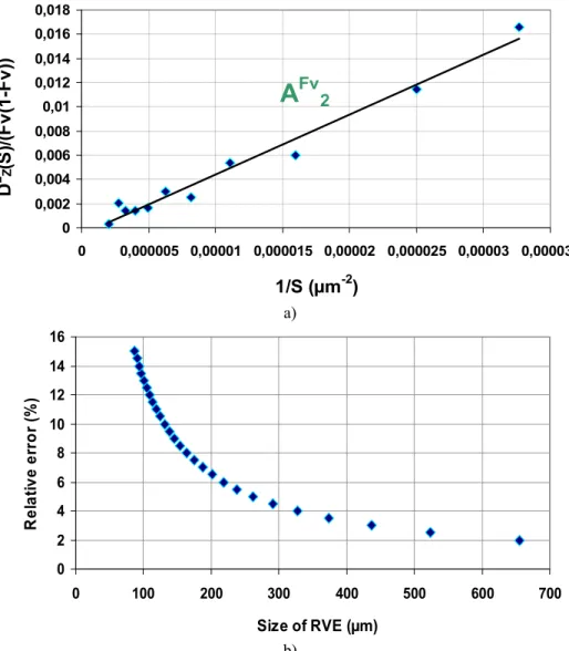
The integral range is deduced from the slope of the curve which relates the variance and the inverse of the area (see equation (10) and Figure 12-a).
A
Fv2 0 0,002 0,004 0,006 0,008 0,01 0,012 0,014 0,016 0,018 0 0,000005 0,00001 0,000015 0,00002 0,000025 0,00003 0,0000351/S (µm
-2)
D
2 Z(S
)/
(Fv
(1
-F
v
))
a) 0 2 4 6 8 10 12 14 16 0 100 200 300 400 500 600 700 Size of RVE (µm) R e la ti ve e rr o r (%) b)Figure 12. a) The integral range of the area fraction; b) RVE according to the relative error Table 5. The RVE of the area fraction according to the relative error for 100 images
Relative error (%) 1 2 3 4 5 8 10 15
Size of RVE
The integral range isA2FV =55´55mm2. It is smaller than the smallest size of images used in this study (50´50
pixels = 122´122mm2), which validates the use of the asymptotic relation (see equation (5)) to compute the variance of estimation. One can observe that the choice of the RVE depends on the desired accuracy (Figure 12-b). In Table 5 some values of RVE are given for various relative precisions and for 100 images. It is instructive to compare our results to those obtained for a carbon-epoxy composite (Thomas et al., 2008): if we consider a single image (n=1) for a 2% and 3% precision, the size are presently 6.56mm
,
and 4.37mm in our case, instead of 611mm and 472mm given in Thomas et al. (2008). This factor ten results from a much higher heterogeneity of the distribution of glass fibers in the present case, due to the presence of layers of resin as shown in Figure 3, resulting in a much higher correlation length deduced from the covariance (typically 600mmas seen on Figure 7-c), instead of 100mm in Thomas et al. (2008).
3.4.6.2 The RVE of the Thermal Conductivity
0 0,001 0,002 0,003 0,004 0,005 0,006 0,007 0,008 0 100 200 300 400 500 600 700 Sqrt (S) (pixels) D 2 Z(S) a)
A
2 0 0,002 0,004 0,006 0,008 0,01 0,012 0,014 0,016 0,018 0,020 2E-06 4E-06 6E-06 8E-06 1E-05 1E-05 1E-05 2E-05 2E-05 1/S (µm-2) D 2 z(S )/D 2 Z b) 0 2 4 6 8 10 12 14 16 0 100 200 300 400 500 600 700 RVE (µm) R e la ti ve e rr o r (%) c) 0,3 0,31 0,32 0,33 0,34 0,35 0,36 0,37 0,38 0,39 0,4 0 200 400 600 800 1000 1200 1400 1600 Sqrt (S) (µm) . גapp (W .m -1 K ) UGT 1UGT 2 d)
Area fraction (%) e)
Figure 13. a) Variance; b) Integral range; c) RVEs according to the relative precision; d) Homogenised conductivities; e) Bounds of Hashin- Shtrikman for S>RVE (for n=100)
By a local post processing, after FEM calculations, the local point variances of different size of images of the microstructure are determined. This enables one to determine the integral range which is equal to
2
2 90 90 m
Al= ´ m . The assumption for the validity of the formula (5) is then satisfied.
To draw the evolution of the RVE (see equation (11)), the local point variance of the large microstructure (1464´1464mm2) is determined (Dl2=3.520972310-2 W
( )
mK -1).The size of the RVE of the thermal conductivity (given for n=100 images) associated to a chosen relative error is given in Table 6. For a single image (n=1) and for 1% of accuracy this size is very large (9.69mm), as compared to the RVE of the thermal conductivity of a carbon–epoxy composite ( 280mm) in Thomas et al (2008) for the same contrast of conductivities between the matrix and the fibers. Again this is a consequence of a much larger correlation length in the present case.
The FEM homogenization makes it possible to choose the RVE, which is the smallest size freed from the effects of the boundary conditions (Figure 13-d), and which is equal to 732´732mm2. Its relative error is 1.32% when using 100 images of this size, and 13.2% for only one image. For images with a larger area the behavior is almost constant and is called effective behavior (Figure 13-d). The fibers, being five times more heat conducting than the matrix, control the effective thermal conductivity. The effective conductivity tensor is given by
( )
1 1 10 44 . 3 0 0 36 . 3 - -ú û ù ê ë é = W mK eff lOne can notice incidently that the effective thermal conductivity shows a slightly anisotropic behavior in the two main directions as a result of a low contrast between the conductivities of the fibers and of the matrix. This difference is of 2%.
In addition, from images larger than the RVE, the thermal conductivity is correctly estimated by the Hashin-Shtrikman lower bound, (Figure 13-e), with less dispersion than in Figure 10 c. A more precise estimation of the thermal conductivity is provided by the 3D Hashin-Shtrikman lower bound (Figure 14).
Table 6. The RVE of the thermal conductivity according to the relative error, for n=100images
Relative error (%) 1 2 3 4 5 8 10 12
Size of RVE
Area fraction (%)
Figure 14. Bounds of Hashin & Shtrikman for S>RVE (for n=100 and 3D analytical formula) 3.4.6.3 RVE of the Elastic Moduli
a) RVE of the Bulk modulus
K 0,E+00 1,E+05 2,E+05 3,E+05 4,E+05 5,E+05 6,E+05 7,E+05 0 100 200 300 400 500 600 700 Sqrt (S) (µm) D 2 Z(S) a) Ak2 0 0,0005 0,001 0,0015 0,002 0,0025 0,003 0,0035 0,004 0,0045
0,E+00 3,E-06 6,E-06 9,E-06 1,E-05 2,E-05 2,E-05
1/S (µm-2) D 2 Z(S )/D 2 Z b) 0 2 4 6 8 10 12 0 100 200 300 400 500 600 700 Size of RVE (µm) R elat iv e error (%) c) 4000 5000 6000 7000 8000 0 250 500 750 1000 1250 1500 Sqrt (S) (µm) K ( M Pa) d)
Area fraction (%) e)
Figure 15. a) Variance; b) Integral range, c) RVEs according to the relative precision, d) Homogenised bulk modulus, e) local bulk modulus estimation for volume larger than the RVE
Table 7. The RVE of the Bulk modulus according to the relative error for n=100 images
Relative error (%) 1 2 3 4 5 8 10 25
Size of RVE11 K
(µm) 1058 530 353 265 212 133 106 43
The bulk modulus local variance is DK2 =58160825MPa. The integral range is A2K=43´43mm2. The size of the RVE of the bulk modulus associated to a chosen relative error is given in Table 7 for 100 images.
By the FEM, as previously seen, we determine the smallest RVE which is not influenced by the effect of boundary conditions (Figure 15-d). It is the RVE of the bulk modulus, and it is equals to 488´488mm2, with an associated relative error of 2.17 % (for n=100 images). While considering only one image of this size, the relative error of this RVE is 21.7%. Its effective value is 5.94GPa.
In Figure 15-e it is observed that the Hashin-Shtrikman bounds estimation is more accurate with image size larger than the RVE for heterogeneous material (see for comparison the Figures 11-c and 11-d). This shows again the paramount importance of the RVE of heterogenous material in the predicting of the macroscopical behavior. This is very useful for mechanical design.
b) RVE of Shear modulus
µ 0,E+00 2,E+05 3,E+05 5,E+05 6,E+05 8,E+05 9,E+05 0 300 600 900 1200 1500 Sqrt (S) (µm) D 2 Z(S) a) Aµ 2 0 0,004 0,008 0,012 0,016 0,02 0 0,0000035 0,000007 0,0000105 0,000014 0,0000175 1/S (µm-2) D 2 Z(S )/D 2 Z b)
0 1,5 3 4,5 6 7,5 9 10,5 0 200 400 600 800 1000 Size of RVE (µm) R e la ti v e e rr o r ( %) c) 4,0E+02 1,0E+03 1,6E+03 2,2E+03 2,8E+03 3,4E+03 0 250 500 750 1000 1250 1500 Sqrt (S) (µm) µ ( M P a) d) Area fraction (%) e)
Figure 16. a) Variance; b) Integral range, c) RVEs according to the precision, d) Homogenised shear modulus, e) local shear modulus estimation for volume larger than the RVE
The local point variance for the transverse shear modulus is Dm2 =5233550MPa. The integral range is 2
2 73 73 m
Am= ´ m .
The size of the RVE of the transverse shear modulus associated to a choosen relative error for 100 images is given in Table 8.
As for the previous steps, the RVE freed from boundary conditions is determined by FEM homogenization, and equals 854´854mm2, with an associated relative error of 1.87% (for 100 images) and 18.7% for only one image. The effective transverse shear modulus of the RVE is 2.1GPa (Figure 16-d).
The shear modulus has the larger RVE, as a result of its strong dependence of the fibers spatial arrangement. Therefore, this RVE will be the final RVE of the studied properties (area fraction, thermal conductivity, bulk modulus, transverse shear modulus). The relative errors induced on every property with this size of RVE for 100 images are given in Table 9.
Table 8. The RVE of the shear modulus according to the relative error for n=100images
Relative error (%) 1 1.5 2 3 4 5 10 11 Size ) ( 11 m RVEm m 1594 1063 797 532 399 319 160 145
4 Comparison between Experimental and Numerical Results
Table 10 provides the comparison between the experimental and the numerical calculations results.
The volume fraction determined by pyrolysis is much closed to the area fraction (2D) provided by image analysis (40 %). This volume fraction is determined before images segmentation for numerical simulations.
The underestimation of the bulk and the shear moduli (Table (10)) by the effective behavior of the RVE can be explained: On one hand, the segmentation has probably reduced the size and the number of fibers, and thus the composite strength in numerical computations. On the other hand, the fibers and matrix input data we used for numerical computations could be underestimated.
However, a comparision between the calculated and the macroscopical thermal conductivity of the composite is not made, since no experimental measurements are available in the present study.
5 Conclusion
Firstly, mechanical tests were performed and the macroscopical elastic behavior is fully characterized by a transversely isotropic stiffness matrix. This is the macroscopical approach. Then we carried out a multi-scale image analysis (microscopical and mesoscopical approach), with a large number of images (100 images with 10 sizes). This step enabled us to highlight the influence of the various fluctuations (local area fraction and fibers spatial arrangement) on the mechanical and thermal behavior of the composite. It showed in addition the need to use a representative volume element (RVE) which takes into account all dispersions (local area fraction, fibers spatial arrangement, etc) for heterogeneous materials.
Several statistical tools such as the integral range and the covariance enabled us to study the evolution of the RVE according to the relative error. However, at this step the effect of boundary conditions on measured property is not known.
The FEM homogenization makes it possible to choose the first volume (area in our case) which is freed from boundary conditions effects and which is the RVE.
Furthermore it is shown that the property which depends strongly on the fiber spatial arrangement requires the larger RVE. This was the case of the shear modulus (854´854mm2, with 1310 fibers). This RVE involves a relative error of 18.7% for one studied image.
The bulk modulus is the least sensitive property to the fibers distribution, with a size of RVE of 488´488mm2. It involves a relative error of 21.7% for one studied image. The RVE of the thermal conductivity is
2 732
732´ mm with 13.2% of relative error for one studied image.
The final RVE for these properties is the higher value of different RVEs (854´854mm2). The effective properties of the RVE are compared to the macroscopical behavior of the composite provided by experimental tests. A relatively good agreement is then established. These results show that the macroscopical behavior of a heterogeneous material can be estimated by the calculation of images of the microstructure.
Table 9. The induced relative error on properties with an RVE size of 854 mm , n=100 Volume
Fraction conductivity Thermal Bulk modulus Shear modulus Relative error
(%) 1.19 1.134 1.24 1.87
Table 10. Comparison between experimental and numerical results with an RVE size of 854 mm
Volume
Fraction conductivity Thermal Bulk modulus (GPa) Shear modulus (GPa)
Experimental 40% - 6.90 2.1
Due to the heterogeneity of the microstructure of the studied material, a total area of around 250 mm must be 2 scanned in the material to estimate its morphological, thermal and elastic properties with a 1% statistical property.
Besides, it appeared that the local conductivity and elastic moduli could be estimated by the lower Hashin-Shtrikman bound, provided the size of images is larger than the RVE.
The slight difference between the local moduli and the Hashin-Shtrikman lower bound could result from the geometry of fibers, which are not exactly circular (Figure 4) as a consequence of the polishing and segmentation process.
The originality of these bound estimation, is that one could predict the local fluctuations of the properties of the composite at different scales from the local fluctuations of the fiber area fraction that can be accessed from image analysis or from non destructive testing, such as ultrasonic measurements made on a much larger scale in Guilleminot et al. (2008).
Acknowledgements: This work was done as a part of the Probadur project. The authors are grateful to the
Institute Carnot M.I.N.E.S for supporting this research and CETIM for providing the material.
References
Andrei A A: Representative volume element size for elastic composites: a numerical study. Journal of the
Mechanics and Physics of Solids, 45, (1997), 1449-1459.
Berggren S A; Lukkassen D; Meidell A; Simula L; Narvik: Some methods for calculating stiffness properties of periodic structures. Applications of mathematics, 2, (2003), 97-110.
Berthelot J M : Matériaux composites. Comportement mécanique et analyse des structures . Editions Tec & doc, (1999), p. 642.
Bhattacharyya A; Lagoudas D C: Effective elastic moduli of two-phase transversely isotropic composites with aligned clustered fibers. Acta Mechanica, 145, (2000), 65-95.
Bunsel A R; Renard J: Fundamentals of fibre reinforcced composite materials. Series in Materials Science and Engineering IoP, (2005) p. 398.
Drugan W J; Willis J R: A micromechanics-based nonlocal constitutive equation and estimates of representative volume element size for elastic composites. Journal of the Mechanics and Physics of Solids , 44, (1996), 497-524. Frank Xu X; Chen X: Stochastic homogenization of random elastic multi-phase composites and size quantification of representative volume element. Mechanics of Materials, 41, (2009), 174-186.
Gitman I M; Askes H; Sluys L J: Representative volume: existence and size determination. Engineering
Fracture Mechanics, 74, (2007), 2518-2534.
Grufman C; Ellyin F: Determining a representative volume element capturing the morphology of fibre reinforced polymer composites. Composite Science and Technology, 67, (2007), 766-775.
Guilleminot J; Soize C; Kondo D; Binetruy C: Theoretical framework and experimental procedure for modeling mesoscopic volume fraction stochastic fluctuations in fiber reinforced composites. International Journal of
Solids and Structures, 45, (2008), 5567–5583
Hashin Z; Shtrikman S: A variational approach to the theory of the elastic behaviour of multiphase materials. J.
Mech. Phys. Solids, 11, (1963), 127-140.
Hill R: Elastic properties of reinforced solids: some theoretical principles. J. Mech. Phys. Solids, 11, (1963), 357-372.
Jan G; Jan Z; Michal S: Quantitative analysis of fiber composite microstructure: Influence of boundary conditions. Probabilistic Engineering Mechanics, 21, (2006), 317-329.
Jeulin D : Modèles morphologiques de structures aléatoires et de changement d’échelle. Doctorat d’Etat thesis,
Caen University, (1991), p. 800, France.
Jeulin D; Ostoja-Starzewski M: Mechanics of random and multiscale microstructures. CISM Courses and
lectures n° 430, Springer, (2001), p. 267.
Jiang M; Alzebdeh K; Jasiuk I; Ostoja-Starzewski M: Scale and boundary conditions effects in elastic properties of random composites. Acta Mechanica, 148, (2001), 63-78.
Jiang M; Jasiuk I; Ostoja-Starzewski M: Apparent thermal conductivity of periodic two-dimensional composites.
Computational Materials Science, 25, (2002), 329-338
Kanit T; Forest S; Galliet I; Mounoury V; Jeulin D: Determination of the size of the representative volume element for random composites : statistical and numerical approach. International Journal of Solids and
Structures, 40, (2003), 3647–3679.
Knight M G; Wrobel L C; Henshall J L: Micromechanical response of fibre-reinforced materials using the boundary element technique. Composite Structures, 62, (2003), 341-352.
Lukkassen D; Persson L E; Wall P: Some engineering and mathematical aspects on the homogenization method.
Composites Engineering, 5, (1995), 519-531.
Matheron G: The theory of regionalized variables and its applications. Publications Centre de morphologie
mathématique, Ecole Nationale Supérieure des Mines de Paris , 5, (1971), p. 207.
Mori T; Tanaka K: Average stress in matrix and average elastic energy of materials with missfitting inclusions.
Acta Metallurgica, 21, (1973), 571–574.
Nemat-Nasser S; Hori M: Micromechanics: overall properties of heterogenous materials. Elsevier, (1999).
Ostoja-Starzewski M: Micromechanics as a basis of stochastic finite elements and differences: An overview.
Appl. Mech. 46, (1993), S136-S147.
Ostoja-Starzewski M: Random fields models of heterogeneous materials. International Journal of Solids and
Structures, 35, (1998), 2429-2455.
Ostoja-Starzewski M: Microstructural randomness versus representative volume element in thermomechanics.
Journal of Applied Mechanics, 69, (2002), 25-35.
Ostoja-Starzewski M: Material spatial randomness: from statistical to representative volume element.
Probabilistic Engineering Mechanics, 21, (2006), 112-132.
Ostoja-Starzewski M: Microstructural ramdomness and scaling in mechanics of materials. CRC Series. Modern
Mechanics And Mathematics, Chapman & Hall/CRC (2007), p. 471.
Segurado J; LIorca J: Computational micromechanics of composites: the effect of particle spatial distribution.
Mechanics of Materials, 38, (2006), 873-883.
Serra J: Image Analysis and Mathematical Morphology . Academic Press, London, (1982).
Shan Z; Gokhale A M: Representative volume element for non-uniform micro-structure. Computational
Materials Science, 24, (2002), 361-379.
Sun C T; Vaidya R S: Prediction of composite properties from a representative volume element. Composites
Science and Technology, 56, (1996), 171-179.
Swan C; Kosaka I: Voigt-Reuss topology optimization for structures with linear elastic material behaviours.
Thomas M; Boyard N; Perez L; Jarny Y; Delaunay D: Representative volume element of anisotropic unidirectional carbon-epoxy composite with high-fibre volume fraction. Composites Science and Technology, 68, (2008), 3184-3192.
Torquato S: Random heterogeneous media: microstructure and improved bounds on effective properties. Applied
Mechanics Reviews, 44, (1991), 37–76.
Trias D; Costa J; Turon A; Hurtado J E: Determination of the critical size of a statistical representative volume element (SRVE) for carbon reinforced polymers. Acta materialia, 54, (2006), 3471-3484.
Willis J R: Variational and related methods for the overall properties of composites. Advances in Applied
Mechanics, 21, (1981), 1–78
Xiangdong D; Ostoja-Starzewski M: On the scaling from statistical to representative volume element in thermoelasticity of random materials. Networks and Heterogeneous Media, 1, (2006), 259-274.
Zeman J; Sejnoha M: From random microstructures to representative volume elements. Modelling and
Simulation in Materials Science Engineering, 15, (2007), S325-S335.
Adresses:
Mamane M. Oumarou
Ecole des Mines de Paris, Centre des matériaux, UMR CNRS 7633, BP 87, 91003 Evry Cedex, France mamane.oumarou@mines-paristech.fr
Dominique Jeulin, Professor
Mines Paristech, Centre de Morphologie Mathématique, 35 rue St Honoré, 77300 Fontainebleau, France dominique.jeulin@mines-paristech.fr
Jacques Renard, Professor
Ecole des Mines de Paris, Centre des matériaux, UMR CNRS 7633, BP 87, 91003 Evry Cedex, France jacques.renard@mines-paristech.fr
Philippe Castaing, PhD
CETIM, Centre Technique des Industries Mécaniques, 74 Route Joneliere, 44000 Nantes, France philippe.castaing@cetim.fr