Fast propagation in reaction-diffusion equations with fractional diffusion
Texte intégral
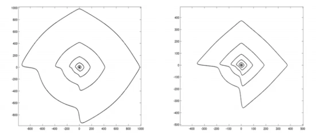
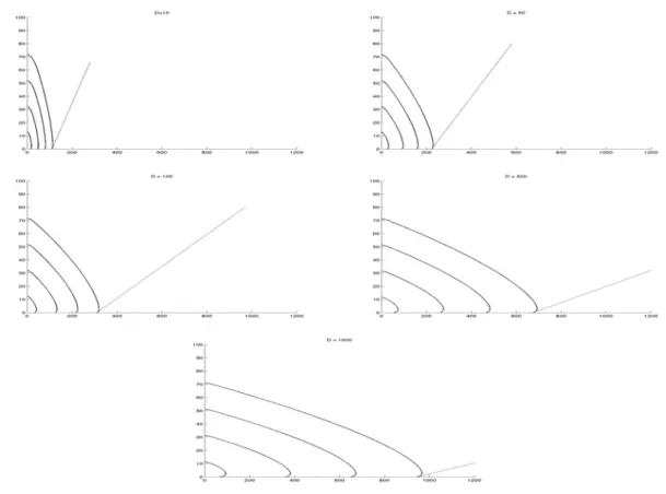
Figure


Documents relatifs
Matching of asymptotic expansions for the wave propagation in media with thin slot – p.11/29.. The different steps of
In this way, using a WKB ansatz, we obtain a Hamilton-Jacobi equation in the limit which describes the asymptotic dynamics of the solutions, similarly to the case of
This paper is concerned with the inverse problem of determining the time and space dependent source term of diffusion equations with constant-order time-fractional deriv- ative in
SOUGANIDIS, A PDE Approach to Certain Large Deviation Problems for Systems of Parabolic Equations, A.N.L., Contributions en l’honneur de J.-J. SOUGANIDIS, The Allen-Cahn
A case with homogeneity: fast diffusion (and porous media) equations Sharp rates of decay of solutions to the nonlinear fast diffusion equation via functional inequalities.. More
In Section 6, the τ -monotonicity in time, for any τ > 0, is shown in the region where u is close to 0, by using some Gaussian estimates as well as some new quantitative
The existence of pulsating traveling waves has been proved by Nolen, Rudd and Xin [17] and the first author [15] under various hypotheses in the more general framework of space-
• In the last section we first study numerically the existence of a speed threshold such that the population survives if c is below this threshold, i.e the solution of the
