THE NUMERICAL SOLUTION OF THE HEAT DIFFUSION EQUATION VIA LATTICE BOLTZMANN METHOD

THE NUMERICAL SOLUTION

OF

THE HEAT DIFFUSION

EQUATION VIA LATTICE BOLTZMANN METHOD

A.ATIA12- and

K.MOHAMMEDF

tUniversité d'El-Oued ,

B.P

789, 39000 El-Oued, Algerie 2

Laborqtoire Energétique - Mécanique

&

Ingénieries

(LEMI),

Université

M'Hamed

Bougara, 35000 Boumerdes, Algerie *E-mail _{: [email protected]}

Abstract.

In

the

present

work,

the solution

of

the

heat

diffusion problem

is

presented using lattice Boltzmann method

(LBM).

The

two

dimensional task is considered and the different boundary conditions, specifically the

Dirichlet

and Neumann are taken

into

account. The D2Q4 lattice model

is

applied.

To

check the accuracy

of

the

LBM

algorithm, the same problems have been solved using the

explicit

variant

of

the

finite

difference method. In the

final

paft of the paper, the results of computations are shown and the conclusions are formulated.

Keywords:

lattice Boltzmann method, numerical solution,

diffusion

equation

INTRODUCTION

Over

the

last decade

the

lattice Boltzmann method

(LBM)

has been developed as a

promising

computational

tool

to

analyze

the

large

class

of

engineering problems, among others, the heat transfer problems. M.Bittagopal

and

C. Mishra

_[1]

applied the

LBM

to

solve the energy equations

of

conduction-radiation problems on non-uniform

lattices.

H.

Shokouhmand

et

al

_[2]

studied

fully

developed

laminar

flow

and convective heat transfer between two parallel plates. R.Chaabane et

_{al [3]}

investigated the solution of conduction problems

with

heat

flux

boundary condition.

In

the

present study,

the

simplest

model D2Q4

BGK

was chosen

to

solve

the

heat

diffusion

equation in 2D square domain

with

different boundary condition.

In

the

absence

ol

convection and

radiation,

for

a 2-D

Cartesian geometry, energy equation is given by:

ar

/a2T

a2r\

o

*=

a\*z+

un')*

_*

Where

_{a =}

j1is

the thermal

diffusivity.

pc

(1)

q,k,

p

and

c

are the rate

of

heat generation

per unit

volume, thermal conductivity

of

the

medium, density

and

specific

heat, respectively.

T,x,t

denole

the

temperature,

spatial

co-ordinates

and time,

respectively.

The equation (1) is supplemented by boundary conditions:

IInitial

condition,t =

0,

T(x.y,0)

-

0"C

I

uft

ttd",,

=

o, ?'(0,ÿ,

t) =

100'c

)aisnt

tfi",*

=

t,

r(t.y,t)

=

o"C

(Z)

I

eouo

side,y ₌

ç,

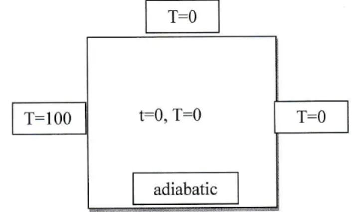
ufrt*,0,11 -- o"C (adiabattc condilion)

Fig. 1

A

square (2D) domain

with

coordinate system

FORMULATION AND KINETIC EQUATION

The

starting

point

of

the

LBM

is

the

kinetic

equation

which

for

a

2-D

geometry is given

_{by [4]:}

âf,(r

t\

:1r)-z+ëi.Vfi7,t)-Ai i-1,,2,3,...m

(3)

ot

where

_fi

is the

particle

distribution function

denoting the number

of

particles at the lattice node

I

₌

(r(x,

y,

z))

at

time

t

moving

in

direction

i

with

velocitye â1 along the

lattice

link

Lr

₌

etLt

connecting

the

nearest neighbors

and

m

is

the

number

of

directions

in

a

lattice through

which

the

information

propagates. The

term collision

operator

Oi

represents

the rate

of

change

of

fi

due

to

collisions. The

discrete Boltzmann equation

with

Bhatanagar-Cross-Krook

(BGK)

approximation is given

by

[4,

s]:

%P+

ë1.vfi@,t)

=

_{-';v,rr,r1- f:"ù?,t)l}

Where

r

is the relaxation time

and;(ea)

i,

11r" equilibrium distribution function. For a

given

application, relaxation

time

r

is

different

for

difierent

lattices. The relaxation time

r

for the D2Q4 lattice is computed

from

_[6]:

2.a.At

7

, - _-r_

_"-

_Lxz

_'2

(s)

For the D2Q4 laltice, the four velocities

ë;

and

their coresponding

weights

w;

are

calculated

from

_[6]:

ë,

:

(1,0). c

è,

_-

(-1,0).c

â,

=

(0,1).c

ën

_-

(0,-1).c

and

w1=

Wz

₌

Wz

₌

w4

_-

0.25

(4)

(6)

€3 e, e2 e4

It

is to

be

noted

that

in

the

above

equation, c

_-

A,x/Lt

₌

Ay/Lt

and

the

weights satisfy the relation

)ll,

w;

₌

1

After

discretization in 2D, and considering heat generation, Eq. (3) can be

written

as:

fi@

+

A.x,y

+

Ly,t

+

Lt) =

fiQ,y,t)[1

-

ar]

+

afr"q(x,y,t)

+

wi.Lt.s

(7)

Where S

_-

_,a

_pc is the force or source term,

wi

is the weight

in

corresponding direction, and

t)

₌

₌

_a is non-dimensional relaxation time. Notice that the

unit

of

S is the

unit

of

temperature

('C)

per unit of time.

This is

the

LB

equation

with BGK

approximation that describes the evolution

of

the particle

distribution

function

_fi.

The solution

of

the above equation

by

LBM

consists of

two

steps, collision and streaming _[6]:

The

collision

step is:

fi?,

y,

t

+

^r)

:

_fi@,

y,

t)lL

_-

al

+

a _{fr"q (x, y,}

t)

+

_wi.

Lt. S

The streaming step is:

fi@

+

Lx,y

+

Ly,t

+

Lt)

=

fi@,y,t

+

At)

In

case

ofheat

transfer problems, the temperature is obtained after summing

_f;

overall direction [7]:

4

r(x,y,t)

_-\ft{x,t,t)

(B)

i=1

To

process

Eq.

(7),

an

equilibrium distribution function

is

required.

For

heat conduction problems, this is given by:

lfq@,y,t)

=

wi.T(x,y,t)

(9)

From

Eqs. (8) to (9), we also have

444

\

f:

o

f*, r,

r>

₌

lw

t.

r

@,

t, t)

:

r

@, y,

t)

=

|

f,

@,

t,

t)

i=1

i=1

i=1

(10)

Eq.

(10),

with

definitions

of

temperaturc

T(x,y,t)

and

equilibrium

function \r"q

(x,y,t)

given

in

Eqs. (8) and (9), respectively, provide solution

ofa

transient heat conduction problem in the

LBM.

BOUNDARY CONDITIONS

FOR

LATTICE BOLTZMANN METHOI)

In the

following

subsection, different boundary conditions

will

be discussed in detail.

l.

The value of the

function

(temperatue) is given at the

boundary:

For

example, temperature

at the

left,

upper and

right

boundaries are

given,

T:Cl:

100'C

atx

₌

0,

and

T:C2:0'C

at.

y

-

h

and

x

= l,

(C1

and

C2

are constants), so

from Eq. (8):

(f,(0,t,t)

+

_fr(o,y,t)

+

_fr(o,y,t)

+

_fn@,y,t)

-r

_-

ct:100"c

atx:o

lh{r,n,t)+

fz?.h,t)+

ft(x,h,t)+

fq(x,h,t):T

-

c2-0 aty=h

(11)

lhQ,y,t)+

fz(t,y,t)+

fr(t,y,t)+

fn(l,y,t)

-r

-

c2=0 atx=t

Then,

the

unknowns

are

_fr(O,y,t)

and

fr(O,y,t)

for left

boundary,

right boundary, because the other distribution functions can be obtained

from

steaming

step.

fr(O,y,t)

and.

_ft(O,y,t)

can be calculated by using

flux

conservation equation _[6]:

fr"q(o,y,t)- fr(o,y,t)+

fr"q(o,y,t)-

fz@,y,t)

_-o

(12)

Since w;

₌

0.25

for

all

steaming

direction

and,

_fr"q

(O,y,t)

_-

_fzeq

(O,y,t)

:

O.

2sT:0.2sC1

(fom

Eq. (9)),then

_{fr(O,y,t) =}

0.25C1.

+

0.25CL

_-

_f2(0,y,t),

so:

fr(o,y,t):

0.5c1

_-

_fz(o,y,t)

_-

50

_-

fz(o,y,t)

(13)

Similarly

we can obtain:

fr(x,h,t)

_-

s0

_-

_1z(0,y,t)

(14)

Hence t\À/o _{unknowns are specified at the}

_left

_{boundary, similar method can be applied}

for

other

boundaries.

The

conditions

for

other

boundaries

will

be

given

in

the

following

equations without derivations,

following

the same procedure as before.

F

upper boundary

(f1@,h,t)

_-

_{0.sCz- fz@,h,t)}

r---

_'"".'.:,

₍₁₅₎

lf+(x,

h,

t)

:

o.sc2

_-

_fr(x,

h,

t)

F

right

boundary

(fr(t,Y,t)

:0.5C2

_-

_fr(t,y,t)

tr,itl,r:,ri

_-

o.sc2

-'iitl,y,a

(16)

2.

adiabatic

boundary condition:

ff:

0: By using

finite

difference approach.

fr

=

0..*

be approximated as

T (x .y + 1,t) _-T (x,y _,t)

___:_____:-

₌

_u

\77

)

Ly

It

can

simplified

asT(x,y +

1,

t)

-

T(x,y,t),

hence for bottom boundary

y =

Q;

fr(x,

t,

t)

+

fz@, 7,

t)

₊

_ft(x,

7,

t)

_{+ f+(x,}

7,

t)

=

_fr(x,o,t)

+

_f2Q,0,t)

+

_fr(x,o,t)

+

fn@,o,t)

(18)

It

is rational to assume that

_f1@,L,t)

*

_h@,0,t),

_f2@,1,,t)

_-

_fr(x,0,t)

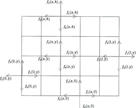
and so on.

f,(x' h) fi(o'y) 1,(',à) în@,h) hQ, l.t@,y) t f,(x'v) 1,(Lv) î,

h(0!)

(/,)) f"(x' v) f,

c,»

f"(L,v) ) 1^(o,v) fz@'o)

t

Â(r o)

f,e'

h@,0)

Fig. 3 Lattices for 2-D diffusion problem

with

distribution function at the boundarv

f,(x' h

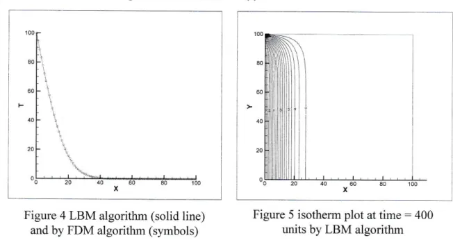
RI,SULTS

OF

COMPUTATIONS

A

two

dimensional squa-re

slab shown

in

fig.1

subjected

to

a different

boundary conditions. The length

of

the domain

is

100

units.

the temperature

distribution in

the

slab

obtained

at time

:

400 units (s),

by

using

LB

and

FD

methods. Thermal

diffusivity is

0.25.

Note that

for

stabiiity

conditions

the

time

step

for FDM is

0.2. There is no such a problem

in

using a time step

of

1.0

with

the

LBM

method. Hence,

LBM

is much faster and efficient than FDM.

Figure

2

illustrate the

temperature

distributions

obtained

by

LBM

algorithm

(solid

line)

and

by FDM

algorithm (symbols) along the

middle line

(y:0.5 H),

where

H

is the high

ofthe

square.

Figure 3 shows the isotherm plot at time

:400

units (s)

Figure 4

LBM

algorithm (solid line) and by

FDM

algorithm (symbols)

20

Figure 5 isotherm plot at time

:

400 units by

LBM

algorithm

CONCLUSION

The lattice Boltzmann method

for

the 2D heat

diffusion

equation supplemented by different boundary conditions and

initial

condition has been presented. The exemplary tasks have been solved

both

by the

lattice Boltzmann

method and

by the

explicit

scheme

of

the

finite

different method. The good agreement

of

the solutions obtained

has been observed.

RE,FERENCES

B. Mondal and S. C. Mishra, "Lâttice Boltzmann method applied to the solution ofthe energy equations

of the transient conduction and radiation problems on non-uniform lattices." International Journal of

Hedt and Mass Ttct sfer, voJ. 51, pp. 68-82. 2008.

H. Shokouhrnand. F. Jam, and M. Salimpour, "Simulation oflaminar flow and convective heat tratsfer in conduits filled \ÿith porous media using Lattice Boltzmann MÈthod." lnternarional Co nluûicdtions i

Heat and Mass Transfer- vol. 36. pp.378-3 84. 2009.

lll

30

2A

I t-t3l t4l t5l t61 t7l

R. Chaabane, F. Askri, and S. B. Nasrallah, "Application ofthe lattice Boltzmann method for solving conduction problems with heat flux boundary condition," presented at International Renewable Erergy

Congress, Sousse Tunisia, 2009.

S. Stcci, The laxice Boltznxann equatlon: _/tr JILlid dynaulcs and belolxd: Oxford university press, 2001. P. L. Bhatnagar, E. P. Cross, and M. Krook, "A model for collisioû processes in gases. I. Small âmp;itude

processes in charged and neutral one-component systems," Pàlsica I review, vol.94, pp. 511, 1954.

A. A. Mohamad, Lattice Boltzrûann method: _{l:itndatnentals and engineering applications} ÿith computer

codes: Springer. 201l.

W.-S. Jiaung, J.-R. Ho, and C.-P. Kuo, "Lattice Boltzmann method for the heat conduction prob)em with phase change." Nnnrerical Heat Tt'ansfer: Part B: Fundanxentals, vol. 39, pp. 167-181.2001.