HAL Id: hal-01159024
https://hal.inria.fr/hal-01159024
Submitted on 2 Jun 2015
HAL is a multi-disciplinary open access
archive for the deposit and dissemination of
sci-entific research documents, whether they are
pub-lished or not. The documents may come from
teaching and research institutions in France or
abroad, or from public or private research centers.
L’archive ouverte pluridisciplinaire HAL, est
destinée au dépôt et à la diffusion de documents
scientifiques de niveau recherche, publiés ou non,
émanant des établissements d’enseignement et de
recherche français ou étrangers, des laboratoires
publics ou privés.
Heterogeneous Resource Selection for Arbitrary HPC
Applications in the Cloud
Anca Iordache, Eliya Buyukkaya, Guillaume Pierre
To cite this version:
Anca Iordache, Eliya Buyukkaya, Guillaume Pierre. Heterogeneous Resource Selection for Arbitrary
HPC Applications in the Cloud. 15th IFIP International Conference on Distributed Applications and
Interoperable Systems (DAIS), Jun 2015, Grenoble, France. pp.108-123,
�10.1007/978-3-319-19129-4_9�. �hal-01159024�
Heterogeneous Resource Selection for
Arbitrary HPC Applications in the Cloud
Anca Iordache, Eliya Buyukkaya, and Guillaume Pierre
IRISA - University of Rennes 1
Abstract. Cloud infrastructures offer a wide variety of resources to choose from. However, most cloud users ignore the potential benefits of dynamically choosing cloud resources among a wide variety of VM instance types with different con-figuration/cost tradeoffs. We propose to automate the choice of resources that should be assigned to arbitrary non-interactive applications. During the first ex-ecutions of the application, the system tries various resource configurations and builds a custom performance model for this application. Thereafter, cloud users can specify their execution time or financial cost constraints, and let the system automatically select the resources which best satisfy this constraint.
1
Introduction
Cloud computing offers unprecedented levels of flexibility to efficiently deploy de-manding applications. Cloud users have access to a large variety of computing resources with various combinations of configurations and prices. This allows them in principle to use the exact type and number of resources their application needs. However, this flexibility also comes as a curse as choosing the best resource configuration for an ap-plication becomes extremely difficult: cloud users often find it very hard to accurately estimate the requirements of complex applications [1].
Most cloud applications are either long-running service-oriented applications, or batch jobs which perform a computation with no user interaction during execution. Batch applications may use frameworks such as MapReduce, or simply behave as black-boxes executing arbitrary operations. Although frameworks such as Elastic MapReduce allow users to dynamically vary the number of resources assigned to a computation [2, 3], other types of HPC applications require that the resource configuration must be cho-sen prior to execution – and kept unchanged during the entire computation.
Selecting the “right” set of resources for an arbitrary application requires a detailed understanding of the relationship between resource specifications and the performance the application will have using these resources. This is hard because the space of all pos-sible resource configurations one may choose from can be extremely large. For example, Amazon EC2 currently offers 29 different instance types. An application requiring just
five nodes must therefore choose one out of 295= 20, 511, 149 possible configurations.
Furthermore, users’ expectations may be more complex than executing the applica-tion as fast as possible: the fastest execuapplica-tion may require expensive resources. Depend-ing on the circumstances, a user may therefore want to choose the fastest option, the cheapest, or any option implementing a tradeoff between these two extremes.
We propose to automate the choice of resources that should be assigned to arbitrary non-interactive applications that get executed repeatedly. Upon the first few executions of the application, the system tries a different resource configuration for each execu-tion. It then uses the resulting execution times and costs to build a custom performance
model for the concerned application. After this phase, users can simply specify the exe-cution time or the financial cost they can tolerate for each exeexe-cution, and let the system automatically find the resource configuration which best satisfies this constraint.
The system indifferently supports single– and multithreaded applications built around frameworks such as MPI and OpenMP. Its only assumption is that the execution time and cost are independent from the application’s input. Although slightly limiting, this assumption is met in a number of HPC applications which are optimized to perform high-volume, repetitive tasks where successive executions process inputs with the same size and runtime behavior. This is the case in particular of the two real-world applica-tions we use in our evaluaapplica-tions (one in the domain of oil exploration, the other in the domain of high-performance database maintenance).
Allowing the automatic selection of computing resources for arbitrary batch cloud applications requires one to address a number of challenges. First, we need to describe arbitrary applications in such a way that a generic application manager can automate the choice of resources that the application may use. Second, we need an efficient search strategy to quickly identify the resource configurations that should be tested. Finally, we need to generate performance models that easily allow one to choose resources according to the performance/cost expectations of the users.
We propose four configuration selection strategies respectively based on uniform search of the configuration space, resource utilization optimization, simulated annealing and a resource utilization-driven simulated annealing. Evaluations show that the latter strategy identifies interesting configurations faster than the others.
Section 2 discusses related work. Section 3 shows how to abstract arbitrary applica-tions in a single generic framework. Secapplica-tions 4, 5 and 6 respectively present the system architecture, its profiling strategies, and their evaluation. Finally, Section 7 concludes.
2
Related Work
In HPC, most performance modeling techniques can be classified into analytical predic-tive methods, code analysis or profiling [4, 5]. Analytical methods require developers to provide a model of their application. They can be very accurate, but building good models is labor-intensive and hard to automate. Moreover, user estimates of application runtimes are often highly inaccurate [1]. Code analysis automates this process, but it usually restricts itself to coarse-grained decisions such as the choice of the best accel-eration device for optimizing performance [6].
In cloud environments, performance modeling was studied for specific types of ap-plications such as Web apap-plications. Besides the numerous techniques which dynami-cally vary the number of identidynami-cally-configured resources to follow the request work-load, one can use machine learning techniques over historical traces in order to define horizontal and vertical scaling rules to handle various types of workloads [7]. Similarly, when scaling decisions are necessary, one may dynamically choose the best resource type based on short-term traffic predictions [8]. Some other works exploit the fact that identically-configured cloud resources often exhibit heterogeneous performance [9]. For instance, one can benchmark the performance of each individual virtual machine instance before deciding how it can best be used in the application [10, 11].
Performance modeling has been addressed for specific types of scientific applica-tions. For bags-of-tasks applications, one can observe the statistical distribution of task
execution times, and automatically derive task scheduling strategies to execute the bag under certain time and cost constraints [12]. Similar work has also been realized for MapReduce applications [13, 14].
For arbitrary HPC applications which do not fit the MapReduce or the bags-of-tasks models, the only solution currently proposed by Amazon EC2 is to empirically try a va-riety of instance types and choose the one which works best [15]. CopperEgg automates this process by monitoring the resource usage of an arbitrary application over a 24-hour period before suggesting an appropriate instance type to support this workload [16]. However, as we shall see in Section 6, utilization-based methodologies do not neces-sarily lead to optimal results. Besides, CopperEgg does not allow the user to choose her preferred optimization criterion. Our work, in contrast, aims at finding Pareto-optimal configurations for arbitrary batch applications, and it supports the automatic selection of resources which match a given optimization criterion.
3
Handling arbitrary applications
Each time a user wants to launch the application, she provides a Service-Level Objec-tive (SLO) taking one of two forms: either impose a maximum execution cost while requesting to execute as fast as possible; or impose a maximum execution time while minimizing the cost of the execution. The system is in charge of automatically selecting the resource configuration which best satisfies this SLO.
To allow a generic application manager to handle arbitrary batch applications, each SLO file contains a link to an Application Manifest which describes the application’s structure and the type of resources it depends on to execute correctly. The manifest is typically written by the application developer.
Figure 1 shows a simple example which describes the types of resources an ap-plication needs, with their number, configuration and role. The Configuration attribute describes the properties that resources may have. A computing resource may thus for example specify a number of cores and memory size, while a storage resource may describe properties such as the disk size and supported IOPS. Each field may specify either a fixed value, or a set of acceptable values to choose from.
We do not specify the network capacity between provisioned machine instances in
our manifests, as current clouds do not allow a user to specify such properties 1. A
logical extension of this work would be to also specify available bandwidth between resources, provided that the underlying cloud can take such requests into account.
Finally, one can assign a Role to a resource. This allows us to describe applica-tions with multiple components potentially having specific requirements. For example, a master/slave application may separately describe Master and Slave resources.
4
System Model
This section introduces our system model supporting the automatic management of batch applications under user objectives. In the following, we explain the architecture of our system and the profiling policies we employ.
1
Amazon EC2 lets users choose a network performance level among ‘Low’, ‘Moderate’, ‘High’ and ‘10 Gigabit.’ However, these qualifiers do not imply any clear guarantees on the resulting available bandwidth.
ApplicationName: HelloWorld ...
Resources { Resource1 (
Type: Virtual Machine Role: Worker Number: 1 Configuration: { Cores: {1..16} Memory: {2,4,6,8,12, 16,24,48,64,96,124} }), ... }
Fig. 1: Application Manifest Example
Application Manager
Dynamic Resource Scheduler
Manifest + SLOs + VM VM ... VM User Model (Performance, Cost) Execute Application Execution Manager Configuration Designer Profiler Controller Provision Configuration
Fig. 2: System Overview
4.1 Architecture
Our system architecture is depicted in Figure 2. A user triggers an execution of the application by submitting an SLO and its associated manifest file to the application manager.
The application manager is an application-agnostic component in charge of choos-ing and provisionchoos-ing the resource configurations, deploychoos-ing and executchoos-ing the applica-tion and of measuring the execuapplica-tion time and implied cost. Initially, it has no knowledge about the types of resources it should choose for a newly-submitted application. After loading the manifest file, in case no performance model is specified, the Controller for-wards the application to the Profiler which executes the application repeatedly using a different resource configuration every time. Note that it is important for our system that execution times should be as deterministic as possible. We therefore need to rely on the cloud to minimize interferences with other co-located instances.
This profiling process continues until either a predefined number of executions has been performed or a profiling budget has been exceeded. The result of these executions (cost and execution time) is used to build a performance model which is sent to the Configuration Designer. If a performance model was already specified in the manifest, the Controller skips the Profiler and sends the application and its model directly to the Configuration Designer. Based on this model, the Configuration Designer then selects a configuration that satisfies the SLO and launches the execution. In both cases, the execution is handled by the Execution Manager which provisions the configuration through a Dynamic Resource Scheduler and finally executes the application on it.
Each time an application execution is performed, the system monitors its total ex-ecution time and cost, and derives a relation between them and the resource configu-ration. Failed executions due to a cloud failure are re-launched on identical configured resources while executions failed due to unmet application requirements are assigned a very high execution time/cost, making them unselectable in the future.
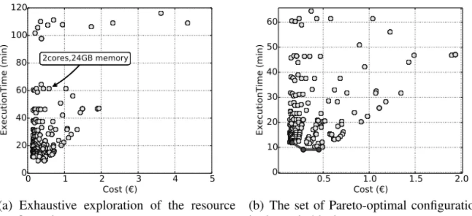
The results generated after several executions with various resource configurations can be plotted as shown in Figure 3(a). Each point represents the execution time and cost that are incurred by one particular resource configuration. The figure shows the
result of an exhaustive exploration of a search space with 176 possible configurations. In a more challenging scenario the number of configurations would be much greater, and this type of exhaustive exploration would be practically unfeasible.
4.2 Pareto Frontier
It is interesting to notice that not all configurations provide interesting properties. Re-gardless of the application, a user is always interested in minimizing the execution time,
the financial cost, or a trade-off between the two2.
Figure 3 presents the search space of the “RTM” application used later in the evalua-tion. Configurations which appear at the top-right of the figure are both slow and expen-sive. Such configurations can be discarded as soon as we discover another configuration which is both faster and cheaper. The remaining configurations form the Pareto frontier of the explored search space. Figure 3(b) highlights the set of Pareto-optimal points of this application: they all implement interesting tradeoffs between performance and cost: points on the top-left represent inexpensive-but-slow configurations, while points on the bottom-right represent fast-but-expensive configurations.
The Pareto frontier (and the set of configurations leading to these points) forms the performance model that the application manager uses to choose configurations satisfy-ing the user’s SLOs. If an SLO imposes a maximum execution time, the system discards the Pareto configurations which are too slow, and selects the cheapest remaining one. Conversely, if the SLO imposes a maximum cost, it discards the Pareto configurations which are too expensive, and selects the fastest remaining one.
4.3 Profiling Policies
Profiling an application requires one to execute it a number of times in order to measure is performance and cost using various resource configurations. This process may be realized in two different ways, depending on the user’s preferences:
1. The offline approach triggers artificial executions of the application whose only purpose is to generate a performance model. In this case, the output of executions is simply discarded.
2. The online approach opportunistically uses the first actual executions requested by the user to try various resource configurations and lazily build a performance model.
Choosing one of these approaches requires the user to make a simple tradeoff. In offline profiling, the user will incur delays and costs of the profiling executions before a performance model has been built. On the other hand, all the subsequent executions will benefit from a complete performance model. In online profiling, although the first executions may not fulfill their SLO until a performance model has been built, the overall marginal cost and delays will be reduced.
2
An interesting extension of this work would be to consider additional evaluation metrics such as carbon footprint. This can be easily done as long as the relevant metrics are designed such that a lower value indicates a better evaluation.
0 1 2 3 4 5 Cost ( ) 0 20 40 60 80 100 120 ExecutionTime (min) 2cores,24GB memory 2cores,24GB memory 2cores,24GB memory 2cores,24GB memory 2cores,24GB memory 2cores,24GB memory
(a) Exhaustive exploration of the resource configuration space 0.5 1.0 1.5 2.0 Cost ( ) 0 10 20 30 40 50 60 ExecutionTime (min)
(b) The set of Pareto-optimal configurations is shown in black
Fig. 3: Resource configuration space of the RTM application.
5
Performance Profiling
The main issue when building the performance model of an application is that the space of all possible configurations is usually much too large to allow an exhaustive explo-ration. We therefore need to carefully choose which configurations should be tested, such that we identify the optimal configurations as quickly as possible.
5.1 Search Space
The search space of resource configurations to explore for an application is generated using the application manifest. Each resource parameter which should be chosen by the platform constitutes one dimension of the space. The number of possible configurations therefore increases exponentially as new dimensions are added, an issue often referred to as the curse of dimensionality.
In the example from Figure 1, the search space of the application has 2 dimensions (corresponding to numbers of cores and memory). This creates a total of 16 × 11 = 176 possible configurations (due to 16 possible numbers of cores, and 11 possible memory sizes). Within these 176 configurations, only a subset of them may offer interesting tradeoffs between performance and cost.
5.2 Search Strategies
The goal of the profiling process is to search through the space of possible configura-tions and to quickly identify configuraconfigura-tions that implement interesting performance/cost tradeoffs. It aims not only to find the fastest or the cheapest configuration but also con-figurations which offer interesting tradeoffs between these two extremes.
We define four strategies that can be used to explore a configuration space: Uniform Search strategy explores stepwise points in the resource search space to select a configuration for the profiling process. As shown in Algorithm 1, the application is executed for all combinations of stepwise resource values (lines 2-5). Although uniform
Algorithm 1 Uniform Search
Input: Application A, Resources R = {R1, R2, ..., Rn}
Output: Set of configurations, their execution time and cost Sr,t,c
1: Sr,t,c← ∅
2: for r1= min1to max1by step1do
3: for r2= min2to max2by step2do
4: ...
5: for rn= minnto maxnby stepndo
6: r ← {r1, r2, ..., rn}
7: (t, c) ← execution time and cost of running A on r
8: Sr,t,c← Sr,t,c∪ {(r, t, c)}
9: ...
Algorithm 2 Utilization-Driven
Input: Application A, Resources R = {R1, R2, ..., Rn}
Output: Set of configurations, their execution time and cost Sr,t,c
1: r ← {r1, r2, ..., rn} where riis a uniform random sample of Ri∈ R
2: Q ← {r} 3: Sr,t,c← ∅
4: while Q 6= ∅ do 5: r ← dequeue(Q)
6: (t, c) ← execution time and cost of running A with resource configuration r 7: Sr,t,c← Sr,t,c∪ {(r, t, c)}
8: for i = 1 to |R| do
9: if Riis over- or underutilized then
10: if Riis overutilized then
11: r0i← next value of Ri(value after ri)
12: else if Riis underutilized then
13: r0i← previous value of Ri(value before ri)
14: enqueue(Q, {r1, r2, ..., ri0, ..., rn})
search is extremely simple, it may waste time exploring large areas which are unlikely to deliver interesting performance/cost tradeoffs. In addition, low exploration step values result in high complexity, while using high step values (to decrease the complexity) may skip relevant configurations.
Utilization-Driven strategy is a simplified version of the CopperEgg strategy [16]. It iteratively refines an initial resource configuration by monitoring the resource utilization generated by the application. As shown in Algorithm 2, the algorithm starts with a random resource configuration (lines 1-2), and monitors the utilization of each resource type in configurations (lines 8-9). If a resource is highly used by the application, the algorithm then allocates a higher amount of this resource in the hope of delivering better performance (lines 10-11). On the other hand, if a resource utilization is low, the algorithm then reduces this resource amount in the hope of reducing resource costs (lines 12-13). Otherwise, it stops its exploration once there is no configuration that neither overuses nor underuses its resources. This strategy is simple and intuitive but, as we shall see later, it may stop prematurely whenever it reaches a local minimum in the search space.
Algorithm 3 Standard SA
Input: Application A, Resources R, Temperatures Tcoolingand Tcurrent
Output: Set of configurations, their execution time and cost Sr,t,c
1: r ← {r1, r2, ..., rn} , riis random value of resource Ri∈ R
2: (t, c) ← execution time and cost of running A with resource configuration r 3: Sr,t,c← {(r, t, c)}
4: while Tcurrent> Tcoolingdo
5: rnew← neighbor(r, Tcurrent)
6: (tnew, cnew) ← execution time and cost of running A with resource configuration rnew
7: Sr,t,c← Sr,t,c∪ {(rnew, tnew, cnew)}
8: if P robabilityAcceptance((t, c), (tnew, cnew), Tcurrent) > random() then
9: r, t, c ← rnew, tnew, cnew
10: decrease Tcurrent
neighbor(r, Tcurrent)
1: σ ← min(sqrt(Tcurrent), (upper − lower)/(3 ∗ ratelearn))
2: updates ← random.N ormal(0, σ, size(r)) 3: rnew← r + updates ∗ ratelearn
4: return rnew
Standard Simulated Annealing (SA) is a well known generic algorithm for global optimization problems [17]. It initially tries a wide variety of configurations, then grad-ually focuses its search around configurations that were already found to be interesting. To control how many bad configurations are accepted as interesting, it relies on a global time-varying parameter called the temperature.
Algorithm 3 shows the SA routine applied to the resource configurations. The al-gorithm starts with a random resource configuration (line 1), and explores new con-figurations in the neighborhood of the current configuration (line 5). The neighbor() function determines a new configuration by drawing random values around the current
configuration using a normal distribution determined by the temperature. ratelearnis a
scale constant for adjusting updates and upper and lower are the parameter r’s interval bounds. The temperature decreases gradually (line 10), which means that the algorithm accepts new configurations to explore with slowly decreasing probability (lines 8-10). Due to its convergence to optimal solution in a fixed amount of time, simulated anneal-ing quickly explores the search space, focusanneal-ing most of its efforts in the “interestanneal-ing” parts of the search space.
In order for the algorithm to explore configurations that are both cost-efficient and performance-efficient, we evaluate each configuration based on the product between the cost and the execution time it generates.The minimization of the product is guarantee-ing the minimization of at least one of them. Usguarantee-ing this utility function the algorithm explores the entire Pareto frontier, instead of focusing on optimizing only the execution time or the cost.
Directed Simulated Annealing is a variant of the previous algorithm. As shown in Al-gorithm 4, the difference lies in the implementation of the neighbor() function: instead of choosing configurations randomly around the current best one, Directed Simulated Annealing uses resource utilization information to drive the search towards better con-figurations. If a resource is under-utilized (resp. over-utilized), Directed SA increases
Algorithm 4 N eighborDirectedSA(r, Tcurrent)
1: if P robabilitydirected< random() then
2: for i = 1 to |R| do
3: if riis over- or underutilized then
4: if riis overutilized then
5: σ ← 1 − ri
6: rnewi← ri+ random.N ormal(0, σ, 1)
7: else if riis underutilized then
8: σ ← ri
9: rnewi← ri+ random.N ormal(0, σ, 1)
10: else
11: rnewi← ri
12: if no update has been done then 13: rnew← neighbor(r, Tcurrent)
14: else
15: rnew← neighbor(r, Tcurrent)
16: return rnew
(resp. decreases) this resource value by a random amount. Otherwise, if the monitoring data cannot offer any direction to drive the search, Directed SA updates the resource value in any direction. This strategy can therefore be seen as a combination of the Utilization-Driven and the Standard Simulated Annealing strategies.
6
Evaluation
This section evaluates the search strategies presented in the previous section. We fo-cus on three evaluation criteria: (i) the convergence speed of different search strategies towards identifying the full set of Pareto-optimal configurations; (ii) the quality of con-figurations we can derive from these results when facing various SLO requirements; and (iii) the costs and delays imposed by offline vs. online profiling.
We base our evaluations on two real HPC applications:
– Reverse Time Migration (RTM) is a computationally-intensive algorithm used in the domain of computational seismography for creating 3D models of underground geological structures [18]. It is typically used by oil exploration companies to re-peatedly analyze the geology of fixed-sized areas. We use a multithreaded, single-node implementation of this application.
– Delta Merge (DM) is a re-implementation of an important maintenance process in the SAP HANA in-memory database [19]. This operation is used to merge a table snapshot with subsequent update operations (which are kept separately) in order to generate a new snapshot. For consistency reasons the database table must remain locked during the entire operation. It is therefore important to minimize the execution time of Delta-Merge as much as possible.
Both application manifests define resource configurations between 1 and 16 CPU cores and 11 discrete values between 2 and 124 GB of memory. We simplify the RTM case by imposing a CPU frequency of 2.2 GHz for the physical machine hosting the VMs, while for DM we authorize 4 possible values. This creates a relatively small
0.0 0.1 0.2 Cost ( )0.3 0.4 0.5 0.6 0 20 40 60 80 100 ExecutionTime (min) 1 Core(s),2GB Mem 16 Core(s),124GB Mem 3 Core(s),6GB Mem 1 Core(s),2GB Mem Uniform Search Utilization Driven Standard SA Directed SA
(a) RTM after 1 execution
0.0 0.1 0.2 Cost ( )0.3 0.4 0.5 0.6 0 20 40 60 80 100 ExecutionTime (min) (b) RTM after 10 executions 0.0 0.1 0.2 Cost ( )0.3 0.4 0.5 0.6 0 10 20 30 40 50 60 ExecutionTime (min) (c) RTM after 20 executions 0.000 0.01 Cost ( )0.02 0.03 0.04 1 2 3 4 5 6 7 ExecutionTime (min) 1 Core(s),2.0GHz,6GB Mem 8 Core(s),2.2GHz,24GB Mem 5 Core(s),2.93GHz,12GB Mem 6 Core(s),2.4GHz,16GB Mem (d) DM after 1 execution 0.000 0.01 Cost ( )0.02 0.03 0.04 1 2 3 4 5 6 7 ExecutionTime (min)
(e) DM after 10 executions
0.000 0.01 Cost ( )0.02 0.03 0.04 1 2 3 4 5 6 7 ExecutionTime (min) (f) DM after 20 executions
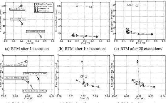
Fig. 4: Pareto frontiers for RTM (a,b,c) and DM (d,e,f).
search space with 172 configurations for RTM and a significantly larger one for DM. Figure 3 shows the result of this exhaustive evaluation for RTM.
We run experiments in the Grid’5000 testbed [20]. For RTM, we use machines equipped with two 10-core CPUs running at 2.2 GHz, 128 GB of RAM and 10 Gb Eth-ernet connectivity. Additional machines with different CPU frequency, number of cores and amount of memory are used for executing the DM application.
All machines run a 64-bit Debian Squeeze 6.0 operating system with the Linux-2.6.32-5-amd64 kernel. We use QEMU/KVM version 0.12.5 as the hypervisor. We de-ploy the OpenNebula cloud infrastructure in these machines so our application manager can request dynamic VM configurations via the OCCI interface. We repeated all exper-iments three times, and kept the average values for execution time.
As our applications typically run within tens of minutes, we define execution costs for resources on a per-minute basis according to a simple cost model derived from a linear regression over the price of cloud resources at Amazon EC2:
CostV M = 0.0396 ∗ NCores+ 0.0186 ∗ NM emory(GB)+ 0.0417
When using cores of different frequency, the cost is scaled accordingly. Note that our system does not rely on this simplistic cost model. It is general enough to accept any other function capable of giving a cost for any VM configuration.
6.1 Convergence speed
To understand which search strategy identifies efficient configurations faster, we com-pute the Pareto frontiers generated by each strategy after 10 and 20 executions. The results are presented in Figure 4.
In the case of Uniform Search, we use a step equal to the unit for each dimension of the search space. It therefore actually completes an exhaustive search of the configura-tion space. We can observe that this strategy converges very slowly. It eventually finds the full Pareto frontier, but only after it completes its exhaustive space exploration.
The Utilization-Driven strategy starts from a randomly generated configuration in the search space. This randomly-chosen starting point creates a different search path for each run of this strategy. In the worst case, this strategy starts with a configuration which neither over- nor underutilizes its resources, so the search stops after a single run. In the best case, the algorithm starts from a configuration already very close to the Pareto frontier, in which case it actually identifies a number of good configurations. We show here an average case (neither the best nor the worst we have observed): it quickly identifies a few interesting configurations but then stops prematurely so it does not identify the entire frontier.
Finally, Standard SA and Directed SA also start from randomly generated configu-rations. We can however observe that they converge faster than the others towards the actual Pareto frontier. For both applications, after just 10 iterations they already iden-tified many interesting configurations. We can note that Directed SA converges faster than Standard SA.
6.2 SLO Satisfaction Ratio
Another important aspect of the search result is the range of SLO requirements it can fulfill, and the quality of the configurations that will be chosen by the platform under these SLOs. We now compare the quality of solutions proposed by the different search strategies after having had the opportunity to issue just 10 profiling executions.
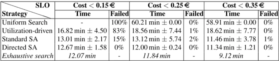
Table 1 presents the execution times that would be observed with the RTM appli-cation if the SLO imposed various values of maximum cost. Several search techniques rely on random behavior so we compute the average and standard deviations of 100 runs of each profiling technique. We also show the number of runs where the strategy failed to propose a configuration for a given SLO. Conversely, Table 2 shows the costs that would be obtained with the RTM application after defining a maximum execution time. For both tables we also show the performance that would result from an exhaustive search of the entire space. Tables 3 and 4 show similar results for the DM application.
It is clear from all the tables that Directed SA provides better configurations. With its good approximation of the entire Pareto frontier, it can handle all SLOs from the table. The other strategies have only a partial or sub-optimal frontier and cannot find configurations for demanding SLOs. At the same time, when several strategies can pro-pose solutions that match the SLO constraint, the solutions found by Directed Simulated Annealing are almost always better, with a lower standard deviation.
6.3 Profiling Costs
Another important aspect is the time and cost incurred by the profiling process which can be minimized based on user’s choice on profiling approach:offline or online.
Table 5 presents the cost and duration overhead of offline profiling for the RTM application using 20 experiments. The utilization-driven strategy appears to be cheap and fast, but this is only due to the fact that it stops after a small number of iterations.
P P P P P PP Strategy
SLO Cost < 0.15e Cost < 0.25e Cost < 0.35e Time Failed Time Failed Time Failed Uniform Search - 100% 60.21 min ± 0.00 0% 58.91 min ± 0.00 0% Utilization-driven 16.82 min ± 4.50 83% 18.56 min ± 7.44 1% 18.62 min ± 7.77 0% Standard SA 13.01 min ± 2.17 15% 13.12 min ± 5.74 2% 11.46 min ± 3.78 1% Directed SA 12.67 min ± 1.58 0% 12.00 min ± 0.24 0% 11.34 min ± 1.21 0% Exhaustive search 12.07 min - 11.84 min - 9.12 min
-Table 1: Performance after 10 executions of RTM under cost (C) constraints. The values correspond to the average and standard deviation of 100 runs of the search techniques. P P P P P PP Strategy
SLO Time < 10.00 min Time < 20.00 min Time< 30.00 min Cost Failed Cost Failed Cost Failed
Uniform Search - 100% - 100% - 100%
Utilization-driven 0.28e ± 0.00 98% 0.16e ± 0.01 33% 0.17e ± 0.05 6% Standard SA 0.35e ± 0.08 36% 0.16e ± 0.05 0% 0.15e ± 0.05 0% Directed SA 0.40e ± 0.08 30% 0.14e ± 0.00 0% 0.14e ± 0.00 0% Exhaustive search 0.28e - 0.13e - 0.13e
-Table 2: Performance after 10 executions of RTM under time (T) constraints. The values correspond to the average and standard deviation of 100 runs of the search techniques. P P P P P PP Strategy
SLO Cost < 0.02e Cost < 0.04e Cost < 0.06e Time Failed Time Failed Time Failed Uniform Search 2.23 min ± 0.00 0% 2.10 min ± 0.00 0% 2.10 min ± 0.00 0% Utilization-driven 2.11 min ± 0.25 74% 2.14 min ± 0.64 22% 2.20 min ± 0.91 12% Standard SA 3.47 min ± 1.42 26% 2.14 min ± 0.92 5% 1.97 min ± 0.63 3% Directed SA 2.62 min ± 1.10 7% 1.66 min ± 0.18 0% 1.60 min ± 0.16 0% Exhaustive search 1.81 min - 1.46 min - 1.46 min
-Table 3: Performance after 10 executions of DM under cost (C) constraints. The values correspond to the average and standard deviation of 100 runs of the search techniques.
PP P P P PP Strategy
SLO Time < 2.00 min Time < 3.00 min Time< 4.00 min Cost Failed Cost Failed Cost Failed Uniform Search - 100% 0.02e ± 0.00 0% 0.02e ± 0.00 0% Utilization-driven 0.03e ± 0.02 49% 0.03e ± 0.02 10% 0.03e ± 0.02 4% Standard SA 0.04e ± 0.02 28% 0.02e ± 0.01 6% 0.02e ± 0.01 1% Directed SA 0.02e ± 0.01 1% 0.02e ± 0.00 0% 0.02e ± 0.00 0% Exhaustive search 0.01e - 0.01e - 0.01e
-Table 4: Performance after 10 executions of DM under time (T) constraints. The values correspond to the average and standard deviation of 100 runs of the search techniques.
Uniform Search starts its exploration from the cheapest available resource types which incur long execution times, thus, the execution becomes expensive.
Standard SA is slightly cheaper and faster than Directed SA mostly due to a an initial temperature chosen too low which means that the algorithm converges quickly before issuing 20 executions (we use the SciPy [21] implementation of SA).
Directed SA does not have this limitation as it does not rely all the time on the temperature to choose a next configuration. This strategy therefore explores more con-figurations, thus having a higher total cost and execution time than Standard SA. On the other hand, it identifies more optimal configurations.
Strategy Total cost Duration Uniform Search 19.92e 1727.93 min Utilization-driven 2.63e 234.51 min
Standard SA 7.09e 426.41 min
Directed SA 9.38e 635.39 min
Table 5: Total cost and duration overhead for an offline profiling of RTM limited to 20 executions. The values represent the average of 100 profiling processes with each search technique. 0 5 10 15 20 0.0 0.1 0.2 0.3 0.4 0.5 0.6 Cost ( ) -0.14 -0.06 +0.68 -0.13 +0.07 -0.16 -0.02 +0.05 -0.10 -0.15 -0.15 -0.16 +0.13 +0.02 -0.05 -0.15 +0.19 +0.15 -0.08 -0.15 SLO : Cost <= 0.3 0 5 10 15 20 Execution 0 10 20 30 40 50 60 ExecutionTime (min) -10.43 +1.23 -7.58 -16.39 +34.42 -16.43 -20.88 +80.11 +71.68 +1.79 +15.75 -17.93 -19.48 -17.83 -14.05 -14.87 -19.84 -20.90 -12.24 -16.95
SLO : Time <= 30.0 min
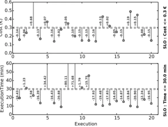
Fig. 5: Cost and Execution Time fluctuation in an online profiling of RTM limited to 20 executions.
Figure 5 shows the execution times and costs incurred by the user using the Di-rected Simulated Annealing strategy in conjunction with online profiling. In this case, no artificial execution is generated. On the other hand, as we can see in the figure, many
executions violate an arbitrary SLO of 0.30e. However, it is interesting to notice that
the overall group of execution remains within its aggregated budget (with a negative
cost overhead of -0.21e). Similarly, when applying an arbitrary SLO of 30 minutes of
execution time, numerous individual executions violate the SLO but overall the execu-tion time overhead is again negative (-20.82 minutes).
We conclude that the search based on Directed Simulated Annealing shows the fastest convergence to optimal configurations and provides a better satisfaction for the SLOs. It generates good configurations to be used when creating an application profile in a smaller number of executions.
For users willing to tolerate SLO violations on individual executions, the online pro-filing strategy provides obvious benefits: it remains within the aggregate time or budget of the overall profiling phase, and therefore offers fast and cost-effective generation of a full performance model. On the other hand users unwilling or unable to tolerate individual SLO violations can revert to the offline strategy, at the expense of artificial executions which consume both time and money.
7
Conclusion
Assigning the appropriate computational resources for efficient execution of arbitrary cloud applications is a difficult problem. We presented an automatic profiling
method-ology that allows a application-agnostic platform to select resources according to an SLO.
Our work so far relies on the assumption that execution time and cost are indepen-dent from the input. The next step in our agenda consists in modeling applications with input-dependent performance.
Acknowledgments. This work was partially funded by the FP7 Programme of the
Euro-pean Commission in the context of the Harness project under Grant Agreement 318521. Experiments were carried out using the Grid’5000 experimental testbed, developed un-der the INRIA ALADDIN development action with support from CNRS, RENATER and several Universities as well as other funding bodies.
References
1. Tang, W., Desai, N., Buettner, D., Lan, Z.: Job scheduling with adjusted runtime estimates on production supercomputers. Elsevier Journal of Parallel and Distributed Computing (2013) 2. Amazon Elastic MapReduce. http://aws.amazon.com/elasticmapreduce/ 3. Azure Batch. http://azure.microsoft.com/en-us/services/batch/ 4. Allan, R.: Survey of HPC performance modelling and prediction tools. Technical Report
DL-TR-2010-006, Science and Technology Facilities Council (July 2009)
5. Pllana, S., Brandic, I., Benkner, S.: A survey of the state of the art in performance modeling and prediction of parallel and distributed computing systems. IJCIR 4(1) (2008)
6. Beach, T.H., Rana, O.F., Avis, N.J.: Integrating acceleration devices using CometCloud. In: Proc. ORMaCloud workshop. (June 2013)
7. Vasic, N., Novakovic, D., Miucin, S., Kostic, D., Bianchini, R.: DejaVu: Accelerating re-source allocation in virtualized environments. In: Proc. ACM ASPLOS. (March 2012) 8. Fernandez, H., Pierre, G., Kielmann, T.: Autoscaling Web applications in heterogeneous
cloud infrastructures. In: Proc. IEEE IC2E. (March 2014)
9. Dejun, J., Pierre, G., Chi, C.H.: EC2 performance analysis for resource provisioning of service-oriented applications. In: NFPSLAM-SOC. (November 2009)
10. Dejun, J., Pierre, G., Chi, C.H.: Resource provisioning of Web applications in heterogeneous clouds. In: Proc. USENIX WebApps. (June 2011)
11. Farley, B., Juels, A., Varadarajan, V., Ristenpart, T., Bowers, K.D., Swift, M.M.: More for your money: exploiting performance heterogeneity in public clouds. In: SOCC. (2012) 12. Oprescu, A.M., Kielmann, T., Leahu, H.: Budget estimation and control for bag-of-tasks
scheduling in clouds. Parallel Processing Letters 21(2) (June 2011)
13. Verma, A., Cherkasova, L., Campbell, R.H.: ARIA: automatic resource inference and allo-cation for mapred uce environments. In: Proc. ICAC. (2011)
14. Tian, F., Chen, K.: Towards optimal resource provisioning for running MapReduce programs in public clouds. In: Proc. IEEE CLOUD. (2011)
15. Amazon Web Services. http://aws.amazon.com/blogs/aws/ choosing-the-right-ec2-instance-type-for-your-application/ 16. CopperEgg: AWS sizing tool. http://copperegg.com/aws-sizing-tool/ 17. Wikipedia.org: Simulated annealing
18. CGC: Reverse time migration http://www.cgg.com/default.aspx?cid=2358. 19. Sikka, V., F¨arber, F., Lehner, W., Cha, S.K., Peh, T., Bornh¨ovd, C.: Efficient transaction
processing in SAP HANA database – the end of a column store myth. In: SIGMOD. (2012) 20. Grid’5000. http://www.grid5000.fr/
21. SciPy: http://docs.scipy.org/doc/scipy/reference/generated/ scipy.optimize.anneal.html#scipy.optimize.anneal.