HAL Id: hal-00737660
https://hal-imt.archives-ouvertes.fr/hal-00737660
Submitted on 2 Oct 2012
HAL is a multi-disciplinary open access
archive for the deposit and dissemination of
sci-entific research documents, whether they are
pub-lished or not. The documents may come from
teaching and research institutions in France or
L’archive ouverte pluridisciplinaire HAL, est
destinée au dépôt et à la diffusion de documents
scientifiques de niveau recherche, publiés ou non,
émanant des établissements d’enseignement et de
recherche français ou étrangers, des laboratoires
Cellular Networks
Hany Kamal, Marceau Coupechoux, Philippe Godlewski
To cite this version:
Hany Kamal, Marceau Coupechoux, Philippe Godlewski. Tabu Search for Dynamic Spectrum
Alloca-tion (DSA) in Cellular Networks. TransacAlloca-tions on Emerging TelecommunicaAlloca-tions Technologies, 2012,
23 (6), pp.508-521. �hal-00737660�
Published online in Wiley InterScience
(www.interscience.wiley.com) DOI: 10.1002/ett.000
Tabu Search for Dynamic Spectrum Allocation (DSA) in Cellular Networks
†
Hany Kamal, Marceau Coupechoux
∗, Philippe Godlewski
Telecom ParisTech & CNRS LTCI, France
SUMMARY
In this paper, we present and analyze a Tabu Search (TS) algorithm for Dynamic Spectrum Allocation (DSA) in cellular networks. We study a case where an operator is providing packet services to the end-users. The objective of the cellular operator is to maximize its reward while taking into account the trade-off between the spectrum cost and the revenues obtained from end-users. These revenues are modeled here as an increasing function of the achieved throughput. The cost is proportional to the bandwidth of the spectrum leased to the regulator or some spectrum broker. Results show that the algorithm allows the operator to increase its reward by taking advantage of the spatial and temporal heterogeneities of the traffic in the network, rather than assuming homogeneous traffic for its radio resource allocation. Our TS-based DSA algorithm is efficient in terms of the required memory space and convergence speed. Results show that the algorithm is fast enough to suit a dynamic context. Copyright c 2xxx AEIT
1. Introduction
Due to the spectrum crowd situation and the high demands on spectral resources, spectrum sharing and Dynamic Spectrum Allocation (DSA) techniques have been recent active research topics. The existing spectrum allocation process, denoted as Fixed Spectrum Allocation (FSA), headed for static long term exclusive rights of spectrum
usage [1] and is shown to be inflexible [2]. Spectrum
sharing has been proposed as a promising method for better usage of spectrum. Researchers have worked on spectrum sharing algorithms motivated by the incentives taken by
FCC to promote a better usage of spectrum [3] [4]. For
example, the authors in [5] propose a coordinated DSA
system where a common pool of resources is shared and controlled by a regional spectrum broker.
In this paper, we consider a framework of several operators sharing a common pool of resources or
Coordinated Access Band (CAB) inspired by [5], and we
focus on the strategy of one operator leasing spectrum
∗Correspondence to: Marceau Coupechoux, 46 rue Barrault, Paris,
France. E-mail: [email protected]
†Part of the results presented in this paper have been published in IEEE
WiMob 2010 and IEEE Wireless Days 2010.
from the broker. The operator does not own the spectrum, but rather has to lease it according to the demands in order to provide packet services for the end-users. We are interested in developing a DSA algorithm based on Tabu Search (TS) that provides the number of spectrum blocks to be acquired from the broker, as well as the frequency assignment corresponding to the maximum reward.
Several algorithms have been proposed to solve the Channel Assignment Problem (CAP) in cellular mobile networks, which is known to be NP-complete in many
of its formulations (see e.g [6]). The classical CAP
consists of assigning the channels to the cells within the mobile network while satisfying: (1) interference constraints (co-channel, adjacent channel or both together) and (2) the traffic load demands. The proposed algorithms in the literature could be classified as follows: algorithms
based on heuristic methods [7], others based on genetic
algorithm [8], on graph coloring method [9], and on neural
network methods [10]. Several papers have also studied
frequency assignment using TS algorithm. For example,
the references [11], [12], [13], and [9] make a partial list of
the references proposing TS algorithm to solve the fixed-spectrum CAP.
It is worth mentioning that most of the work done
Copyright c 2xxx AEIT Received
using TS to solve the fixed-spectrum CAP in cellular networks, has focused on circuit switched traffic (i.e. voice
traffic) with application to the GSM networks (see [12] for
example). Treating voice traffic using TS has always been associated with a hard interference requirement: below a certain Carrier to Interference Ratio (CIR) threshold, the service is not accessible, while above this level, there is no significant increase of the service quality. For this reason, previous works have focused on the minimization of the interference (as an objective function), while satisfying the traffic demands. Note that in order to be able to perform the spectrum assignment, in fixed-spectrum CAP problems, it is necessary to know the number of channels required by each cell.
With the increasing demand of packet data services along with the development of new standards supporting packet applications, i.e., LTE and WiMAX, it would be interesting for DSA techniques to take into account the specificities of packet traffic. In contrast with the case of voice traffic, in packet traffic services, we see the interference constraint as a soft interference requirement, where interference can be tolerated without a hard threshold. A higher level of interference however induces a soft degradation of end-users throughput and consequently affects their satisfaction.
Different from references [9], [11], [12] and [13] that
used TS algorithms, we set an objective function of maximizing the operators reward. The reward is computed here as the sum of revenues obtained from end-users minus the spectrum cost. The revenue obtained from a user is in turn an increasing function of its throughput. The cost is proportional to the bandwidth of the spectrum leased to the broker.
In our formulation of the dynamic-CAP for packet service, the operator has no predefined information about the number of frequency blocks required by the cells. Assigning only one, but poorly interfered, block to a given cell might provide higher throughput to the end-users than assigning two (or more) highly interfered blocks. Thus, the operator needs to find a certain level of compromise in
order to maximize its reward (see section2.1.2).
In [9], the authors have used TS method to solve the
minimum interference DSAproblem. Our approach differs
from [9] mainly due to the consideration of packet context.
Consequently our formulation of the objective function, the neighborhood structure, and the tabu list is different and adapted to the packet traffic assumption. The formulations proposed in this paper lead to a simple algorithm that does not require excessive memory space, and suits the implementation in a dynamic context.
In addition, it is worth noting that the framework proposed in this paper is the same as the one presented
in our previous work [14]. In [14] however, we have only
considered the temporal variations of the traffic without any interference consideration and we have proposed in this context optimal, Q-learning based and heuristic methods for the resource allocation problem. In this paper, we extend this work by taking into account both temporal and spatial traffic heterogeneities and interference issues.
Hereafter, we summarize our main contributions with respect to the related TS work: proposing and analyzing a DSA algorithm based on adapted TS method, where (1) we consider packet traffic services, (2) we address the spectrum pricing issue, (3) we set an objective function for maximizing the operators reward, and (4) we introduce adaptations to TS for a dynamic deployment of the algorithm.
We first propose in section 2 a centralized approach
adapted to a cluster made of a finite and limited number of cells. We illustrate in this part how the TS based DSA (TS-DSA) algorithm can take advantage of the traffic heterogeneity in the network, whether the temporal or the spatial heterogeneity. However the TS-DSA algorithm would have a limited performance in case the operator intends to deploy DSA on a larger area containing high number of cells. In this case, the global deployment of the TS-based DSA on the whole Radio Access Network (RAN), in a centralized manner, has its limitation. The higher the number of cells, the higher the number of TS neighbors to be generated. Consequently higher number of iterations will be necessary to explore different solutions
and to reach a good one. In section 3, we thus propose
a distributed algorithm for the operator to overcome the complexity limitation of the TS-based DSA algorithm when it comes to large RANs. The distributed algorithm allows the operator to deploy (execute) the TS-DSA algorithm on small clusters in a consequent manner and according to the events.
2. Tabu Search Based DSA: Centralized Approach In this section, we start by considering a centralized approach for Tabu Search based DSA. A single central entity is able to make the spectrum assignment to each cell of a cluster. We first define the considered network model
(section 2.1). We then describe the proposed TS-DSA
algorithm (section2.2). We finish this section by showing
how our algorithm can benefit from spatial (using a static
approach in section 2.3) and temporal (using dynamic
simulations in section2.4) heterogeneities of the traffic.
2.1. Network Model
2.1.1. System Model: We study DSA on the cell level
and we focus on a mono-operator case. The operator is supposed to deploy one RAN providing packet services to the end-users. The operator does not own the spectrum but rather has to lease it according to the traffic load. The spectrum is leased from a spectrum broker and consists of an integer number of blocks taken from the common
pool, the CAB. Let Fmaxbe the CAB size in number of
frequency blocks.
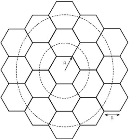
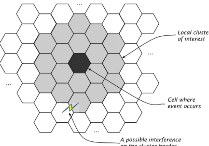
As illustrated in Fig. 1, we are considering a cluster
consisting of one hexagonal central cell and two rings of cells surrounding the central cell. Cells have a radius of R. It is worth mentioning that the usage of an hexagonal model is only for the sake of simple simulations. Our algorithm behaves the same way no matter the type of network topology.
We consider only packet type of service characterized by arrivals and departures of packet calls (we don’t go into the detail of individual packet transmissions). In a given cell, the scheduling is supposed to be fair in throughput. The average data rate accessible by users in a cell is proportional to the bandwidth allocated to the cell and is equally divided among all users of the cell.
!
!
Figure 1. Cluster of a hexagonal network centrally controlled by the DSA algorithm.
2.1.2. DSA Policies: In the considered system model, the
core issue for the operator lies in the trade-off to be found between spectrum cost and revenues obtained from users
[15]. We suppose that a DSA decision is taken by the
operator at each new event, i.e., arrival or departure of a packet call in any cell. A DSA decision assigns spectrum blocks to each cell in the RAN. We assume that at least
one spectrum block is always available to each cell, so that starvation is not possible. This assumption has also a practical reason, when it comes to the implementation of TS algorithm, the research space is indeed decreased.
More formally, a DSA policy can be represented by a
boolean matrixs of size Fmax× B. An element sf cof the
matrix is defined as:
sf c=
(
1, if (frequency) block f is assigned to cell c, 0, otherwise.
According to our convention, none of column vectors ofs
is null. LetS be the set of all possible such matrices. This
is also the set of all DSA policies.
We are interested in the development of a DSA algorithm which maximizes the operators revenue (see
section2.1.4).
2.1.3. CIR and Cell Capacity: Clearly, the bit-rate
obtained by the end-users depends on the perceived Carrier to Interference and Noise Ratio (CINR) level and the CINR level depends on the frequency assignment. The exact CINR distribution in a cell is hard to be determined in practice. For the sake of simplicity, we rely on an approximate calculation for the CINR by focusing on the cell edge, which is a worst case in terms of interference. We consider an urban environment, and hence we neglect the noise and we focus on the CIR. The users are assumed to be located on the cell border and facing the highest level of interference from the interfering cells. We also assume that all cells are transmitting with the same power level. From the previous assumptions, an estimation of the CIR
perceived by the users in cellc on frequency block f given
the DSA policys, is:
CIRfc(s) = sf cmin R−α P i∈Bf(s)\{c}(dc,i− R) −α, CIRmax ! , (1)
whereR is the cell radius, α is the path-loss exponent, dc,i
is the distance between the victim cellc and the interfering
celli, Bf(s) = {j = 1, ..., B s.t. sf j= 1} is set of all cells
using the frequency block f and CIRmax is an upper
bound on CIR. By convention, iff is not allocated to c by
s, the CIR is null. It is worth mentioning that considering different models of the CIR will not affect deeply the proposed algorithm for DSA. All other calculations for CIR can be introduced into the proposed algorithm.
We approximate the cell capacity (in bps) using Shannon classical formula. The cell capacity is the sum of capacities
provided by the frequency blocks used by the cell.
Formally, the cell capacity Cc(s) of cell c under DSA
policys is denoted by:
Cc(s) =
Fmax
X
f=1
Wflog2(1 + CIRcf(s)), (2)
whereWf is the block size in Hz with indexf , CIRcf is
the CIR perceived by cellc on frequency block f . If block
f is not allocated to c by s, CIRf
c(s) = 0 and Cc(s) = 0.
As we consider fair throughput scheduling between users
of a given cell, the data-rateDc(s) obtained by each of the
users in cellc is given by: Dc(s) = Cc(s)/Nc, whereNc
is the number of users in cellc (whenever Nc6= 0).
2.1.4. Reward Model: We give now the reward definition
while taking into consideration both the user date-rate and the spectrum price. The revenue obtained from a given user
in cellc increases with his satisfaction:
φc(Dc(s)) = Ku(1 − exp(−Dc(s)/Dcom)), (3)
where Ku is a constant in euros per unit of satisfaction,
Dcom is a constant called comfort data-rate, and the
satisfaction is an increasing function of the user data rate
(without unit) [16].
Concerning spectrum, we consider the price to be fixed per MHz. The cost paid by the operator for the spectrum can be given as:
KBWfF (s), (4)
where F (s) = |{f = 1, ..., Fmax|∃c, sf c6= 0}| is the
number of frequency blocks used by the RAN given that
DSA policys is used, Wf is the block size in Hz, andKB
is a constant in euros per Hz. Note that a different spectrum price function (for example a function that depends on the
demands in the market as considered in [15] and [17]) can
be used with our algorithm.
The reward obtained by the operator with DSA policys
can thus be written: g(s) =
B X c=1
Ncφc(Dc(s)) − KBWfF (s), (5)
where B is the total number of cells in the cluster
area where DSA is performed. By convention, we set
Ncφc(Dc(s)) = 0 when Nc = 0, i.e., the operator doesn’t
get any reward from cellc when there is no user.
The optimization problem we want to tackle can be written:
max
s∈S g(s). (6)
S being a discrete and finite space, this non linear binary integer programming problem has obviously at least one solution. Finding the optimal solution by brute force may however be cumbersome as the number of cells and spectrum blocks increase.
2.2. Tabu Search Based DSA
In order to maximize the operator reward, we rely on Tabu Search. We first explain the principle of Tabu Search, define the main concepts in our case and detail our implementation.
2.2.1. Principle: Tabu search is a metaheuristic that
guides a local heuristic search procedure to explore the solution space beyond local optimality, by allowing a
degenerated solution [13]. TS was originally presented by
Glover in [18] and [19].
The basic idea is to forbid a move that would return to recently visited solutions by classifying them as tabu.
Hereafter we give the fundamentals of TS. LetS be the
set containing the possible solutions to the problem. For
each solution s ∈ S there exists a subset of S called
neighborhood of s. The neighborhood contains feasible
solutions, each of them is obtained by making a simple
move from the solutions. The algorithm uses a memory
structure called Tabu List (TL) to avoid cycles. The algorithm forbids the selection of a solution among the neighborhood, if this solution have been visited in a previous iteration. At each iteration the TS updates the TL by adding attributes of the selected solution. Note that such attributes do not contain the complete solution otherwise handling the TL will become costly (in terms of required
memory) when the number of iterations increases [13].
Note that the TL has a limited size (called TT for Tabu Tenure) and the choice of the TT has an impact on the obtained result. The smaller the TT, the higher the chance to have cycles (visiting previously visited solutions) and hence TS cannot go beyond the local optimal. However if the TT is very large, very few options will be left for the neighborhood formation, besides the cost for necessary memory space.
The initial point of the TS algorithm has its importance in determining the time (i.e. the number of iterations) required to reach the optimal solution. Starting from a solution very far away from the zone where the optimal solution exists, will require more iterations to explore the different zones. An initialization process aims at facilitating the search procedure for the algorithm, through the reduction of the time required to reach the optimal
solution. Usually an initialization process is based on some heuristic method.
As the minimum number of iterations required to reach an ”efficient” solution using TS is very dependent on the initial start point, the basic idea of TS-based DSA algorithm makes use of this dependency and applies the TS at each new event. A new event does not drastically modify the system state. The previous assignment is thus probably a good starting point for the TS-DSA to find a better solution. In a dynamic context, the algorithm is launched at each new event where it starts from the last reached allocation solution.
2.2.2. Definitions: Before illustrating our implementation
of the TS algorithm, we give the following key definitions. • A solution s is a feasible DSA policy defined as
a Boolean matrix of size Fmax× B such that no
column vector is null (each cell has at least one
block). Taking an example ofFmax= 3 blocks, and
B = 5 cells, then a ”possible” solution s can be given as: s = 1 0 1 0 1 0 1 0 1 1 0 0 0 0 0
In this simple example, only 2 blocks are used by
the RAN (F (s) = 2) and the operator pays for the corresponding spectrum size.
• According to our model, a ”possible” solution means there is at least one block assigned to every cell. Practically, this assumption helps reducing the search space for the algorithm, and hence increasing the chance of reaching a better solution in less number of iterations. The assumption is also realistic because it avoids starvation situations.
• For each solution s ∈ S, we define the set of moves M (s) which can be applied to s in order to obtain a
new solutions′.
• A neighbor s′ of the solution s is created by
applying one movem, where m ∈ M (s).
• The move m is a Boolean matrix of the same size
as s, all its elements equal to zero except one, or
two elements equal to one (see neighbor formation
in section2.3).
• The reward g(s) achieved using a solution s is
calculated as illustrated previously in sections2.1.3
and 2.1.4. The maximum reward ever-reached
during the search process is denotedgmax.
• At each iteration, attributes of the selected solutions are added to the TL.
We have chosen to consider the reward corresponding to each selected solution (among all TS neighbors at each iteration) as its attribute. There is two main advantages
behind this approach: first, adding the rewardg(s) (of the
selected solution s) in the TL, will not only forbid the
TS from selecting s as a valid solution for the following
iterations, but will also forbid visiting all solutions who
achieve the same reward as g(s). The second advantage
is related to the required memory space for the TL. Our TL is composed of a single vector of size TT, each of
its elements being equal to the rewardg(s) corresponding
to the selected solution s. Note that, in our case, g(s)
holds the complete needed information (from the operator
perspective) of the solution matrixs.
2.2.3. Implementation: We present in Algorithm1our TS
algorithm that suits the DSA for packet services.
Algorithm 1 TS algorithm for reward maximization in packet services context
1: Initialization: an initial solutionsinitis found.
2: s ← sinit
3: gmax← g(sinit)
4: while Nb. of iterations≤ MAXITER do
5: Neighborhood formation: all possible TS neighbors
of the initial solutions are created, except those who
are listed as tabu.
6: Neighbor selection: the solution s′ that achieves
the maximum reward is chosen, among the set of
neighbors, with the condition thats′ is not listed
Tabu,s ← s′
7: Tabu list update: the rewardg(s′) corresponding to
the selected solutions′is added to the TL.
8: Maximum reward update: the maximum
ever-obtained rewardgmaxis updated:
ifg(s′) > g
max, thengmax← g(s′) end if
9: end while
2.3. Spatial Heterogeneity
In this section we illustrate the impact of the spatial hetero-geneity of network traffic on algorithms performance.
2.3.1. Implementation Details: We illustrate hereafter the
implementation details of the steps given in Algorithm1
for the first evaluation.
Initialization: We have chosen an initialization method based on randomly formed solutions. Note that the operator does not have clear requirements on the number of blocks
to assign to a cell (unlike [9], [11] and [13]), hence the total number of blocks to be used is unknown to the operator. We divide the search zones according to the total number
of blocks the operator can lease (1, ..., Fmax). Note that the
search zone with a single block is a trivial one because in this case, there is a single possible solution corresponding
to frequency reuse 1. We generate randomly300 possible
solutions for each search zone. The TS algorithm starts using the solution corresponding to the maximum obtained reward among all randomly created solutions.
Neighborhood formation: All possible TS neighbors are created by whether: (1) removing an assigned block from a random cell, (2) adding a non-used block to a random cell, or (3) replacing one of the used blocks in a random cell by a non-used block. Note that adding, removing, or replacing a frequency can be performed by a simple XOR operation.
The neighbor s′= s ⊕ m, where m is a Boolean matrix
that contains zeros except one element equal to one in case of adding or removing a block. In case of replacing a block,
two elements of the matrixm equal to one.
Neighbor selection: According to our defined objective function, the neighbor that achieves the maximum reward among all neighbors is selected.
2.3.2. Simulation Scenarios and Parameters: Hereafter
we define the parameters we used for our simulations. The
maximum number of blocksFmax the operator can lease
is assumed to be6 blocks, with block size Wf of1 MHz.
The comfort bit-rate for the user Dcom = 500 Kbps, the
cell radiusR = 1 Km, and the path-loss exponent α = 3.
The pricing constants are fixed as follows:Ku= 10 euros
andKB= 50 euros/Hz. TS algorithm parameters are set
as follows: Tabu Tenure= 200 and the maximum number
of iterationsMAXITER = 800 iterations.
According to the defined parameter set as well as to the neighbor definition, the total number of possible neighbors
created from a solutions, in the worst case, equals to 285
neighbors. It is clear that, for our case study, generating all possible neighbors at each iteration is very feasible.
Now we are going to use TS to compare the obtained reward through serving a specific amount of traffic load (determined by the total number of active users) in two different cases: (1) the case of an operator using FSA, who assumed a homogeneous traffic over the RAN to perform its channel assignment, and (2) the case of an operator using DSA, who considers the exact (heterogenous) distribution of the traffic to dynamically assign spectrum blocks.
We have first considered a total number of users equal
to 57. We suppose that the distribution of the users is
following a decreasing function of the distance from the central cell. There is a high concentration of users in the central cell (this is the hot spot), and this concentration decreases with the distance from the center of the cluster.
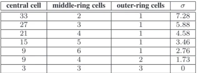
Tab. 1 gives all studied users distributions following this
criterion with a total number of users equals to57 users.
It gives the number of users per cell for the central cell, the middle-ring cells, and the outer-ring cells as well as
the distributions standard-deviationσ. The homogeneous
traffic scenario is also included with its zero standard deviation (all cells have the same number of users).
Table 1. Studied users distributions and corresponding standard deviations σ
central cell middle-ring cells outer-ring cells σ
33 2 1 7.28 27 3 1 5.88 21 4 1 4.58 15 5 1 3.46 9 6 1 2.76 9 4 2 1.73 3 3 3 0
The operator using FSA has assigned frequency blocks to the cells while assuming a homogeneous traffic (last
line of Tab. 1). For a fair comparison, the assignment
is obtained using the TS algorithm but remains fixed whatever the traffic conditions. The operator using DSA adapts its frequency assignment according to the dynamic of the traffic and tries to maximize its reward whatever the heterogeneity situation in the network.
For the sake of comparison, we have then increased the
number of users to152, adding 5 more users to every cells
in all scenarios of Tab.1. The spatial standard deviations
remain unchanged.
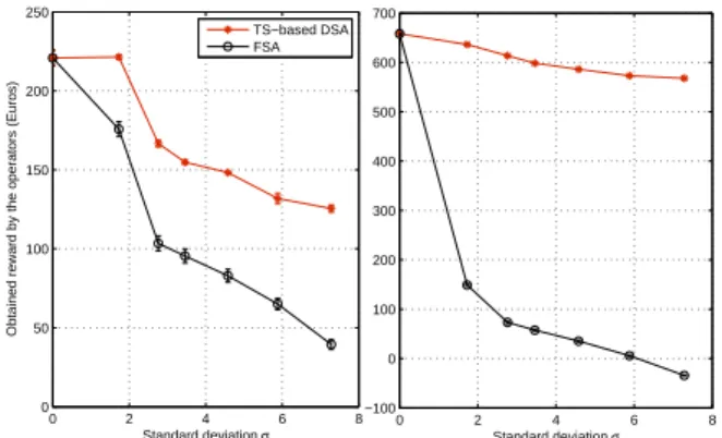
2.3.3. Simulation Results: Fig. 2 gives the obtained
reward versus the standard deviationσ for both operators
for57 (left) and 152 users (right) respectively. Each point
corresponds to a line in Tab.1. Forσ = 0, as both operators
launch the TS algorithm, obtained reward are equal. As heterogeneity grows up (σ increases), the FSA allocation remains the same for the first operator, while for the second, DSA strategy adapts the assignment to the traffic.
We can notice that the obtained reward decreases as σ
increases in all cases, even for the operator who considers the real traffic in the RAN for its resource allocation.
Fig.2shows however that the reward obtained by the DSA
operator exceeds the reward obtained by the FSA operator
for all values ofσ. The same trends can be observed for 57
or152 users.
90% confidence intervals after 10 trials are also shown on the figure. Their small size around the mean value highlights the fact that results are very stable.
0 2 4 6 8 0 50 100 150 200 250 Standard deviation σ
Obtained reward by the operators (Euros)
TS−based DSA FSA 0 2 4 6 8 −100 0 100 200 300 400 500 600 700 Standard deviation σ
Figure 2. Obtained reward by the two operators (using resp. FSA and DSA) as a function of the spatial heterogeneity of the traffic characterized by σ; scenarios with 57 users (left) and 152 users (right).
We give in Fig3a spectrum assignment obtained using
TS-based DSA algorithm for σ = 7.28 and 57 users.
The numbers indicated on the cells represent the block numbers. The TS-based DSA algorithm has assigned one block to all the cells, except the central cell. The algorithm
has assigned3 blocks to the central cell; two of them (block
4 and block 5) are not assigned to any of the other cells,
while the third block (block2) is assigned to some of the
cells on the outer-ring. We see this assignment is coherent with the distribution of users in the cells. Note that the
central cell has33 users (see Table1). The TS used a total
of only5 blocks out of the 6 blocks available (83% of the
CAB is used). For the above scenarios, optimal solution is difficult to obtain. However, we can verify that on small scale scenarios (not shown here) involving e.g. only three cells and six blocks, the TS-based DSA always provides an optimal solution.
2.3.4. Performance of TS: We evaluate in this section
the performance of the TS algorithm in terms of step complexity, memory requirement and convergence time.
The complexity of each step of the TS algorithm resides in the neighborhood formation and reward calculation. According to the neighbor definition, the total number of
possible neighbors created from a solutions equals to:
FmaxB − Bs0+ B X c=1 FcF¯c, (7) !"#$"#%
& & &
& & & ' ' ' ' ' ! ! ! ! ! ! '
Figure 3. Obtained spectrum assignment using TS-based DSA for σ = 7.28.
whereBs0is the number of cells having one block ins, B
is the total number of cells in the RAN,Fc is the number
of frequency blocks used by cellc, and ¯Fc is the number
of blocks not used by cellc. Note that Fc + ¯Fc = Fmax.
The first part of the equation (FmaxB − Bs0) represents
the total number of possible neighbors created due to adding or removing a block from a cell, knowing that at least one block should be assigned to any cell. The summation part represents the total number of possible neighbors created due to the replacement of a block, it is
maximal when∀c, Fc= Fmax/2. So, clearly, the number
of neighbors is in O(BFmax). For each neighbor, the
obtained reward has to be computed. For a given DSA
policys, the CIR computation for one cell is in O(B) (see
Eq.1) and satisfaction inO(BFmax) (see Eq.2and3). As
a consequence, the complexity of the reward calculation
is in O(B2F
max) (see Eq.5). At last, the TS algorithm
complexity is inO(B3F2
max).
The memory requirement of the TS algorithm includes
the Tabu List of size TT float values and O(BFmax)
boolean matrices of sizeB × Fmax.
We now evaluate the performance of our TS algorithm in terms of the number of iterations required to reach an ”efficient” solution. This metric is important from the dynamicity point of view of the algorithm. Note that here and in the rest of the paper, we do not try to necessarily achieve the optimal solution. This would require a unacceptable delay for the operator. We rather
look for a reasonable number of TS iterations that provide a significant gain for the operator.
We assume the same parameter set as given in
section 2.3.2. The RAN has a total number of 57
users. We compare different cases of users distributions: homogeneous and heterogeneous distributions.
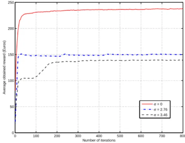
Fig. 4 gives the mean obtained reward using TS as
a function of the number of iterations for σ = 0, 2.76
and 3.46 (see Table 1 for the exact number of users in
each cell). Each of the presented curves in Fig. 4 is the
output of averaging 250 trials. It is clear that the higher
the number of iterations, the higher the chance to get a better solution. A too high number of iterations would however prevent an operator from using the proposed algorithm in a dynamic context. We can further notice
from Fig. 4 that the mean value of the reward increases
with the increase of the iterations number until it stabilizes
(this is true for all values of σ). The minimum number
of iterations required for the mean reward to stabilize is
found to be approximately200, 240, and 320 iterations for
σ = 0, 2.76, and 3.46 respectively. In the homogeneous distribution case (σ = 0) the mean reward curve stabilizes very fast. However in the heterogeneous case, the mean reward curve needs higher number of iterations to stabilize. Obviously, finding the allocation which maximizes the reward in a heterogenous traffic case is more challenging.
0 100 200 300 400 500 600 700 800 0 50 100 150 200 250 Number of iterations
Average obtained reward (Euros)
σ = 0 σ = 2.76 σ = 3.46
Figure 4. Average reward versus the number of iterations.
We can however notice that the required minimum number of iterations is reasonable enough to allow the operator to launch the algorithm at each new event. It is very important to note that the obtained minimum
number of iterationsis very dependent on the initial start
point. In a dynamic context, and at each new event, the
operator is supposed to start TS algorithm from the last reached allocation solution. Hence the minimum number of iterations are expected to be reduced.
For a more efficient algorithm in terms of the convergence speed, we introduce few amendments to the algorithm in the coming section. We also study the temporal heterogeneity of the traffic, and evaluate the network performance while using the amended TS-based DSA algorithm.
2.4. Temporal Heterogeneity
2.4.1. Implementation Details: We begin by giving the
introduced amendments to the implementation of the algorithm to better suit the dynamic context.
Initialization: From our experience, we have noticed that the TS algorithm assigns a number of blocks to each cell that is more or less proportional to the number of users in the cell. Accordingly, we add an amendment to the previously used initialization method making use of this property, to get a good starting solution closer to the zone where the optimal solution exists. As previously, the initialization method is based on randomly formed solutions. We divide the search zones according to
the total number of blocks F the operator can lease,
F ∈ (1, ..., Fmax). We generate randomly 300 possible
solutions for each search zone. However we add the following conditions: (1) only one block is assigned to the cell(s) having one user, (2) a number of blocks equals
to Fmax is assigned to the cell(s) having the maximum
number of users. The TS algorithm starts using the solution corresponding to the maximum obtained reward among all randomly created solutions.
Neighborhood formation: For an efficient algorithm that can be executed at each new event, a limitation of the number of TS neighbors for the first iteration is introduced, depending on the event type (i.e. arrival or departure of a user). The following method is implemented: in case of arrival or departure of a user, replacing one of the used blocks is considered, however: (a) adding a non-used block to a random cell is only considered in case of arrival, and (b) removing an assigned block from a random cell is only considered in case of departure. Note however that, although the number of neighbors is reduced, it is still
inO(BFmax). So the TS algorithm complexity remains
unchanged.
Neighbor selection: In order to choose one neighbor, the operator needs to calculate the reward for all neighbors. This process might affect the efficiency of the algorithm. In order to reduce the algorithms complexity, we introduce
the following method for the selection of cells while calculating the reward for each TS neighbor. For each move that creates a neighbor, only the affected cells by the move are chosen for the reward update. For example, in case of
replacingf5byf4in a cell, then only the cells usingf5or
f4need to be updated.
2.4.2. Simulation Scenario and Parameters: Now we
evaluate the networks performance (algorithms dynam-icity) using event-based simulations. We consider the same RAN topology and size as considered in section
2.3.2. The maximum number of users that each cell
accepts (according to the Connection Admission Control
configuration) equals to 10 users. We assume Poisson
arrivals of packet calls and exponential packet call sizes
(with average3 Mbits). We suppose an heterogenous traffic
in the RAN: there is a high concentration of traffic in the central cell, and this concentration decreases as the distance from the clusters center increases. We assume
the arrival rate for the central cell λ1= 4λ2, whereλ2is
the arrival rate per cell for the cells in the middle-ring,
andλ1= 6λ3, whereλ3is the arrival rate per cell for the
cells in the outer-ring. TS algorithm parameters are set as
follows: the maximum number of iterationsMAXITER =
300 iterations at the very beginning of the TS launch, and 20 iterations at each new event. The presented results are
the average of20000 events.
We compare the reward obtained by two operators; (1) one assumes a homogeneous traffic over the RAN and deploys FSA, and (2) a second operator uses DSA, and considers the exact (heterogenous) distribution of the traffic to dynamically assign spectrum blocks.
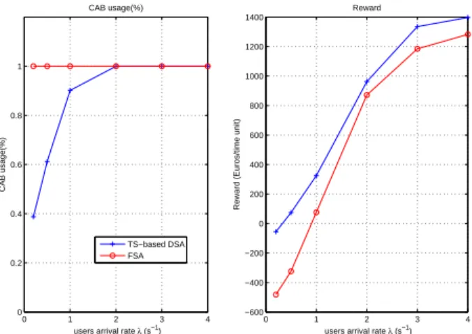
2.4.3. Simulation Results: We compare FSA and
TS-based DSA in terms of the obtained reward, CAB
utilization and the user throughput. Fig. 5 gives the
obtained reward as well as the CAB utilization versus the
mean arrival rateλ using both TS-based DSA and FSA.
We can notice that the obtained rewards using TS-based DSA exceed the rewards obtained using FSA for
all values of simulatedλ, even for 2 ≤ λ ≤ 4s−1 where
both techniques use100% of the CAB. At λ = 1s−1, the
reward obtained using TS-based DSA is334.5 compared to
75.9 using FSA (+345%). We can also see from Fig.5that
a considerable spectrum conservation using the proposed
DSA algorithm is achieved with respect to FSA forλ <
2s−1.
Fig. 6 gives the end-user throughput and the user
satisfaction obtained using both FSA and TS-based DSA. As the FSA uses more spectrum than TS-based DSA,
0 1 2 3 4 0 0.2 0.4 0.6 0.8 1
users arrival rate λ (s−1)
CAB usage(%) CAB usage(%) 0 1 2 3 4 −600 −400 −200 0 200 400 600 800 1000 1200 1400
users arrival rate λ (s−1)
Reward (Euros/time unit)
Reward
TS−based DSA FSA
Figure 5. CAB utilization and obtained reward obtained using FSA and TS-based DSA.
consequently the achieved user throughput and satisfaction are reduced for the DSA case, especially for low values
ofλ. Note that in FSA case a single user in a cell takes
advantage of using2 blocks assigned to the cell, while in
DSA case only 1 block is assigned to the user. Besides,
the interference level generated using regular reuse scheme is indeed different than the one generated due to the deployment of the allocation given by TS-DSA.
0 1 2 3 4 0 0.5 1 1.5 2 2.5 3
users arrival rate λ (s−1)
user bit rate (Mb/s)
User throughput TS−based DSA FSA 0 1 2 3 4 5.5 6 6.5 7 7.5 8 8.5 9 9.5 10
users arrival rate λ (s−1)
user satisfaction
User satisfaction
Figure 6. End-user throughput (left) and user satisfaction (right) obtained using FSA and TS-based DSA.
The promising results observed for a cell cluster lead us to propose a distributed approach of our algorithm more suited to a wide RAN.
3. Tabu Search Based DSA: Distributed Approach We have shown in the previous section that the operator can increase its rewards (over the rewards obtained using FSA) using TS-DSA algorithm by taking advantage of the traffic heterogeneity in the network, whether the temporal or the spatial heterogeneity. However the TS-DSA algorithm would have a limited performance in case the operator intends to deploy DSA on a larger area containing high number of cells.
In this section, we thus propose a distributed algorithm for the operator to overcome the complexity limitation of the TS-based DSA algorithm when it comes to large RANs. The optimization problem remain the same as in the
previous section (see Eq.6), the search spaceS becomes
however very large or even infinite. The distributed algorithm allows the operator to deploy (execute) the TS-DSA algorithm on small clusters in a consequent manner and according to the events. In this section, the distributed TS-DSA algorithm doesn’t aim at finding the optimal solution, it rather provides the operator with a DSA solution that will increase its reward compared to a fixed allocation.
Hereafter we begin by the definition of the distributed approach, we then detail the simulation parameters and scenario and we provide simulation results.
3.1. Distributed TS-DSA
The main idea is to locally run the TS around cells where a packet call is newly initiated or terminated. In a large
RAN containing B hexagonal cells, at each new event
the TS-DSA algorithm, as given in Algorithm1, is to be
launched locally on one cluster C centered on the cell
where the event occurs. Algorithm 1 provides a solution
s∗(C), where s∗(C) is the frequency assignment given
for the local clusterC, while frequency allocation remains
fixed for all cells c /∈ C. Note that the algorithm takes
into consideration the accumulated interference, from allB
cells of the RAN, seen by the users in clusterC. However
the algorithm is allowed to change only the frequency assignment of the cells within the local cluster. A new
constraint concerning the border cells of cluster C is
considered: the solutions∗(C) given by the TS-DSA will
not assign to any of the border cells a frequency that is used
by one of its neighbor cells. Fig 7illustrates the principle
of the distributed model.
In the distributed model, and different from the ”global”
optimization performed on the whole cluster in sections2.3
and2.4, the objective of the TS-DSA is to maximize the
local reward of the concerned cluster. Consequently, (1)
!"#$%&#%'()*+& ",&-.)*+*() /*%%&01*+*& *2*.)&"##'+( 3&4"((-5%*&-.)*+,*+*.#* ".&)1*&#%'()*+&5"+6*+ 777 777 777 777
Figure 7. The local cluster formation in a large RAN.
the revenue part considers only the users in the cluster and (2) the spectrum cost part considers the cost of frequency blocks used only in the cluster (and not in the whole RAN). This way, the TS-DSA is expected to provide a solution
s∗(C) that is using as less frequency blocks as possible.
We give in Algorithm 2 the detailed steps of our
distributed DSA algorithm. As the distributed
TS-DSA algorithm is based on Algorithm1 and as the new
constraint doesn’t significantly modify the complexity, the complexity of the algorithm is unchanged (see
section2.3.4).
Algorithm 2 TS-based DSA algorithm: distributed
1: Initialization: reuse3 frequency assignment scheme
is deployed.
2: At each event: a snap-shot is taken and TS
optimization is performed (using Algorithm 1) on
clusterC centered on the cell where the event occurs,
while taking into consideration the new constraint on the border cells of the cluster.
3: The frequency assignments∗(C) is updated according
to the solution given by Algorithm1.
3.2. Simulation Scenario and Parameters
We consider a RAN withB = 175 cells. The maximum
number of users/cellnmax= 15 users. In order to decrease
the border effects in the simulations, the performance statistics are taken on a group of cells located in the center of the RAN. The number of cells on which statistics are
taken is53. Obtained solutions are expected to be better
when the cluster size increases, since more cells are taken
into account. Choosing large cluster however increases also the convergence time of the algorithm. Based on our preliminary results in the previous section, clusters are made of two cell rings around the cell where an event occurs.
TS-DSA algorithm is launched for 100 iterations for
the first 20 events, then for 20 iterations for the rest of
events. Since the minimum number of iterations required to reach an ”efficient” solution using TS is very dependent on the initial start point, and since we launch TS-based DSA algorithm at each new event (to benefit from this dependency), launching TS for a reasonably high number of iterations at the very beginning will reduce the time needed by TS to converge. The total number of randomly
drawn events is assumed to be10K events. The presented
curves are the average of20 trials. The rest of simulation
parameters are assumed to be the same as given in section
2.3.2.
In order to speed up simulations, we consider in this section a different traffic model than the one presented
in section 2.4.2. For a given cell and at each snap-shot,
a packet call is assumed to arrive randomly according
to a pre-defined probability p and a packet call is
assume to depart with probability1 − p. According to this
assumption, each cell-activity can be modeled as a discrete
time Markov chain withnmax+ 1 states, where nmaxis
the maximum number of users that each cell can accept.
The mean number of usersn in a cell at the steady state¯
can thus be denoted by:
¯
n = ρπ01 − (nmax+ 1)ρ
nmax+ n
maxρ(nmax+1)
(1 − ρ)2 ,
whereρ = 1−pp , andπ0is the probability that the cell has
zero users. ! " ### '$%&(" '$%& ) ) ) ) "() "() "() "()
Figure 8. Traffic model of a cell modeled as a discrete Markov chain.
In the coming section, we evaluate the network performance using the distributed TS-DSA algorithm. We focus on two metrics for the evaluation: first, the percent
gainG in rewards for the operator using the distributed
TS-DSA algorithm over the FSA rewards. The gain is
calculated as:
G =gd− gf
gf
, (8)
wheregd is the reward obtained using the distributed
TS-DSA, andgfis the reward obtained using FSA. The reward
is calculated using the model described in section 2.1.4
over the entire network considered for simulations. Second,
we observe the difference δ in the reward g( ¯C) before
and after the local TS optimization on the cluster, where ¯
C = {c|c /∈ C} is the set of cells in the rest of the network.
We use this metric to determine if the local optimization on one cluster might have a negative impact on the rest of the RAN.
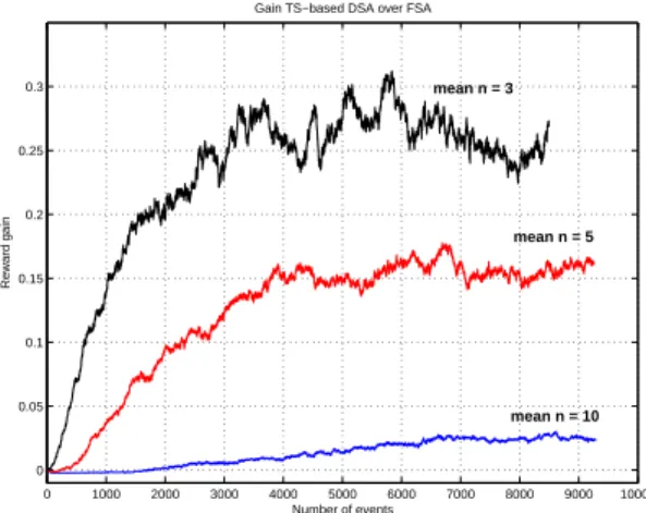
3.3. Simulation Results
Fig.9and Fig.10give the gain in rewards and the standard
deviation of the number of users/cell respectively. Both metrics are plotted as a function of the number of events and for different values of the mean number of users per
celln.¯ 0 1000 2000 3000 4000 5000 6000 7000 8000 9000 10000 0 0.05 0.1 0.15 0.2 0.25 0.3
Gain TS−based DSA over FSA
Number of events
Reward gain
mean n = 10 mean n = 5 mean n = 3
Figure 9. Gain in rewards for the operator at different mean number of users per cell.
We can notice from both figures that the gain in rewards increases in time along with the spatial heterogeneity of the RAN. The users distribution in the RAN, represented by the standard deviation of the number of users per cell, increases in time (with the increase of the number of
events) until it stabilizes, as shown in Fig 10. The same
behavior is noticed for the gainG, as shown in Fig9. This
result is coherent with the one obtained in section2.3(see
Fig2) where TS-DSA is deployed on a RAN of one cluster.
As heterogeneity grows, the gain in reward increases.
0 1000 2000 3000 4000 5000 6000 7000 8000 9000 0 0.5 1 1.5 2 2.5 3 3.5 4 4.5 users distribution σ Number of events User’s standard deviation σ
mean n = 5
mean n = 10
mean n = 3
Figure 10. Standard deviations of the number of users per cell as a function of the number of events.
We can also notice from Fig 9that the gain decreases
with the increase of the traffic load. For mean number of
users per cell ¯n = 3, 5 and 10, the gain G stabilizes at
approximately26%, 15% and 3% respectively.
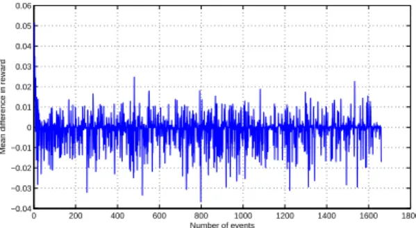
Fig.11gives the difference in rewardsδ as a function
of the number of events forn = 5 users per cell. We can¯
see that the values ofδ are mostly negative values, which
means that a local TS optimization causes reward losses for the rest of the RAN. The reward losses are due to the interference generated from the deployment of the solution F A(C). It is worth mentioning that the negative impact is minor with respect to the gain.
Fig.12gives the gainG values, as a function of the mean
number of usersn. Each point on the bar graph represents¯
the obtained gain value after running the simulations for 2000 events. In this case we reduce the number of events as we use the steady state probabilities at the initialization
step (Algorithm2) to admit a certain number of users to
each of the cells. We can notice that the gain decreases with the increase of traffic load. This result is again not surprising, as the load increases in the network, the reward obtained using DSA converges to the one obtained using FSA.
Finally, Tab.2provides the average simulation duration
of the TS-DSA algorithm as a function of the number
of iterations. The duration for MAXITER = 800 has
been obtained while running the algorithm of section2.3.
MAXITER = 300 corresponds to the initial phase of the
algorithm of section 2.4.MAXITER = 100 corresponds
to the initial phase of the distributed TS-DSA. At last, MAXITER = 20 is the number of iterations used in the
0 200 400 600 800 1000 1200 1400 1600 1800 −0.04 −0.03 −0.02 −0.01 0 0.01 0.02 0.03 0.04 0.05 0.06
Mean difference in reward
Number of events
Figure 11. The difference in rewards δ as a function of the number of events. 2 3 5 7 10 12 0 5 10 15 20 25 30 35
Mean number of users/cell at steady state
Reward gain of TS−DSA over FSA [%]
Figure 12. The gain G in percentage as a function of the mean number of users per cell ¯n.
running phase of the distributed TS-DSA. These figures have been obtained on an average laptop and MATLAB. It is expected that using optimized code and a powerful server would drastically decrease them, so that real-time implementation would be possible.
Table 2. Simulation duration of TS-DSA as a function of the number of iterations. M AX I T ER Simulation duration [s] 20 27 100 85 300 213 800 500
4. Conclusion
In this paper, we have first proposed and analyzed a centralized TS-based DSA algorithm for cellular systems. We have considered a spectrum sharing context while focusing on the strategy adopted by one operator to maximize its reward. We have adapted the TS objective function to suit the packet traffic. We have investigated both the spatial and the temporal heterogeneities of the traffic in the network. Our TS-based DSA algorithm is simple and does not require an excessive memory space. Results have also shown that the algorithm is efficient in terms of the convergence speed. The proposed algorithm allows the operator to increase its rewards and to use less spectrum, however at the price of reduced user throughput. We have then extended the TS-based DSA algorithm using a distributed approach in order to suit the deployment on large RANs. We have evaluated the network performance using two metrics: the gain in rewards with respect to FSA and the effect on the locally optimized clusters. Results have shown that the gain using DSA becomes more interesting when the heterogeneity situations increase in the network. The negative impact on the locally optimized cluster is minor compared to the gain.
REFERENCES
1. M.M. Buddhikot. Understanding dynamic spectrum access: Models,taxonomy and challenges. In New Frontiers in Dynamic
Spectrum Access Networks, 2007. DySPAN 2007. 2nd IEEE
International Symposium on, pages 649 –663, Apr. 2007.
2. T. Kamakaris, M.M. Buddhikot, and R. Iyer. A case for coordinated dynamic spectrum access in cellular networks. In New Frontiers
in Dynamic Spectrum Access Networks, 2005. DySPAN 2005. 2005
First IEEE International Symposium on, pages 289 –298, Nov. 2005.
3. FCC Spectrum Policy Task Force. Report of the Spectrum Efficiency Working Group. Technical report, FCC, 2002. 4. FCC Spectrum Policy Task Force. Report of the Spectrum Rights
and Responsibilities Working Group. Technical report, FCC, 2002. 5. M.M. Buddhikot, P. Kolodzy, S. Miller, K. Ryan, and J. Evans. Dimsumnet: new directions in wireless networking using coor-dinated dynamic spectrum. In World of Wireless Mobile
and Multimedia Networks, 2005. WoWMoM 2005. Sixth IEEE
International Symposium on a, pages 78 – 85, June 2005.
6. W. K. Hale. Frequency assignment: Theory and applications.
Proceedings of the IEEE, 68(12):1497–1514, Dec. 1980.
7. G. Chakraborty. An efficient heuristic algorithm for channel assignment problem in cellular radio networks. Vehicular
Technology, IEEE Transactions on, 50(6):1528 –1539, Nov. 2001.
8. D. Thilakawardana, K. Moessner, and R. Tafazolli. Darwinian approach for dynamic spectrum allocation in next generation systems. Communications, IET, 2(6):827 –836, July 2008. 9. A.P. Subramanian and H. Gupta. Fast spectrum allocation in
coordinated dynamic spectrum access based cellular networks. In New Frontiers in Dynamic Spectrum Access Networks, 2007.
DySPAN 2007. 2nd IEEE International Symposium on, pages 320
–330, Apr. 2007.
10. Yao-Tien Wang and Jang-Ping Sheu. A dynamic channel-borrowing approach with fuzzy logic control in distributed cellular networks.
Simulation Modelling Practice and Theory, 12(3-4):287 – 303,
2004. Modeling and Simulation of Distributed Systems and Networks.
11. Yangjie Peng, Lipo Wang, and Boon Hee Soong. Optimal channel assignment in cellular systems using tabu search. In Personal,
Indoor and Mobile Radio Communications, 2003. PIMRC 2003.
14th IEEE Proceedings on, volume 1, pages 31 – 35 Vol.1, Sept.
2003.
12. R. Montemanni, J.N.J. Moon, and D.H. Smith. An improved tabu search algorithm for the fixed-spectrum frequency-assignment problem. Vehicular Technology, IEEE Transactions on, 52(4):891 – 901, July 2003.
13. A. Capone and M. Trubian. Channel assignment problem in cellular systems: a new model and a tabu search algorithm. Vehicular
Technology, IEEE Transactions on, 48(4):1252 –1260, July 1999.
14. H. Kamal, M. Coupechoux, P. Godlewski, and J.-M. Kelif. Optimal, heuristic and q-learning based dsa policies for cellular networks with coordinated access band. European Transactions on
Telecommunications, 21(8):694–703, 2010.
15. M. Coupechoux, H. Kamal, P. Godlewski, and J.-M. Kelif. Optimal and heuristic dsa policies for cellular networks with coordinated access band. In Wireless Conference, 2009. EW 2009. European, pages 102 –106, May 2009.
16. N. Enderle and X. Lagrange. User satisfaction models and scheduling algorithms for packet-switched services in umts. In
Vehicular Technology Conference, 2003. VTC 2003-Spring. The
57th IEEE Semiannual, volume 3, pages 1704 –1709 vol.3, July
2003.
17. H. Kamal, M. Coupechoux, and P. Godlewski. Inter-operator spectrum sharing for cellular networks using game theory. In
Personal, Indoor and Mobile Radio Communications, 2009 IEEE
20th International Symposium on, pages 425 –429, Sept. 2009.
18. F. Glover. Tabu search - part i. ORSA Journal on Computing, 1(3):190–206, Summer 1989.
19. F. Glover. Tabu search - part ii. ORSA Journal on Computing, 2(1):190–206, Winter 1990.