Maintenance Cost Models

HAL Id: hal-01007484

https://hal.archives-ouvertes.fr/hal-01007484 Submitted on 16 Jun 2014

HAL is a multi-disciplinary open access archive for the deposit and dissemination of sci-entific research documents, whether they are pub-lished or not. The documents may come from teaching and research institutions in France or abroad, or from public or private research centers.

L’archive ouverte pluridisciplinaire HAL, est destinée au dépôt et à la diffusion de documents scientifiques de niveau recherche, publiés ou non, émanant des établissements d’enseignement et de recherche français ou étrangers, des laboratoires publics ou privés.

Distributed under a Creative Commons Attribution| 4.0 International License

Maintenance Cost Models

Alaa Chateauneuf, Franck Schoefs

To cite this version:

Alaa Chateauneuf, Franck Schoefs. Maintenance Cost Models. Judith Baroth; Franck Schoefs; Denys Breysse. Construction Reliability: Safety, Variability and Sustainability, Wiley, pp.271-291, 2012, �10.1002/9781118601099.ch14�. �hal-01007484�

Maintenance Cost Models

14.1. Preventive maintenance

Preventive maintenance allows us to ensure an acceptable level of reliability during the structural lifecycle. A conditional maintenance policy is based on periodic inspections of degradation, which eventurally trigger alarms related to repairs and replacements. In practice, however, quantitative knowledge of the state of degradation and operation conditions presents many uncertainties, which leads to a difficult decision-making process. Therefore, reliability-based maintenance becomes mandatory for decision-making.

The total maintenance cost can be written in the form: REP INS PM F M C C C C C _{= + + +} [14.1]

where C_M is the expected total maintenance cost, C_F is the expected failure cost (including operation losses, production losses, and the direct and indirect damages due to failure), C_PM is the expected preventive maintenance cost, C_INS is the expected inspection cost, and C_REP is the expected repair cost. These costs are affected by uncertainties related to the state of degradation of the structure, the results of inspections and to repair/replacement methods. Moreover, these parameters may vary in terms of socio-economic environment, such as the discount rate, inflation and the fluctuations of market prices.

The failure cost is related to direct damage (human lives, economic losses, loss of benefits, environment degradation, etc.) and to indirect damage (procedure fees, commercial impact, market losses, expert works, long term effects, etc.). Depending on the industry concerned, some costs may increase in an exponential way in terms of the failure rate. For example, the public relations/marketing impact, and therefore market losses, can jump considerably when the number of failed products becomes significant (which is the case in mass production, the automotive industry, aeronautics, etc.) or because the perception of risks makes them unacceptable (which is the case for nuclear power plants, dams, railways, etc.). In energy production industries (e.g. power plants, petro-chemical plants, etc.) the main losses are due to benefit losses when production is stopped. Moreover, during the last decade, the public has become more sensitive to aspects related to the environment; failures inducing pollution are severely punished by justice, politics and public opinion.

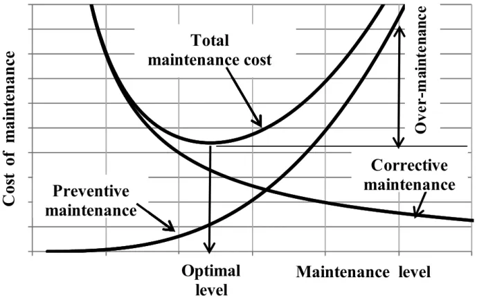
Figure 14.1 illustrates the costs of preventive and corrective maintenance, in terms of the level of planning. A low level of planning leads to larger number of emergency repairs and consequently to a larger total cost. Conversely, a high level of planned maintenance costs more and leads to losses due to over-maintenance. The optimization of the total maintenance cost allows us to find the best equilibrium in terms of the risks to be considered.

Figure 14.1. Illustration of maintenance costs

0 0,1 0,2 0,3 0,4 0,5 0,6 0,7 0,8 0,9 1 0 25 50 75 100 125 150

C

os

t of

m

ai

n

te

n

ance

Maintenance level

Coût total de

maintenance

Coût total de

maintenance

Coût total de

maintenance

Coût total de

maintenance

Coût total de

maintenance

Coût total de

maintenance

Coût total de

maintenance

Total

maintenance cost

Ov er-m ai nt en an ce

Préventive

maintenance

Corrective

maintenance

Optimal

level

For a maintenance cycle

[ ]

0,

_τ

under the assumption of an infinite horizon1, the expectation of the maintenance cost per unit time takes the form:

( )

c f

( )

p ( ) M C P C R C _τ τ τ τ + = [14.2]

where

τ

is the maintenance interval, Cc is the corrective maintenance cost, Cp is the preventive maintenance cost2 and P_f ( )_τ is the accumulated failure probability at

time

τ

; reliability is given by the survival probability R( ) 1_{τ = −}P_f ( )_τ . The choice of maintenance strategy depends on the ratio between preventive and corrective costs; when Cp _<Cc , preventive maintenance becomes useful, otherwise, maintenance should only be performed when the component fails.

14.2. Maintenance based on time

Under this policy, preventive maintenance is performed periodically at predefined times k_τ . When a component fails during an interval

[

(

k ₋1

)

_τ

; k

_τ

]

, corrective maintenance is performed at the failure time. The advantage of this policy lies in its simplicity of application for the management of industrial systems, as preventive maintenance is previously planned and there is no need to monitor the ageing of components. Three versions of the model (I, II, III) can be considered:

– Model I: the failed component is instantaneously replaced when failure occurs; – Model II: the failed component remains unrepaired until the next preventive maintenance;

– Model III: the failed component is subject to minimal repair until the next preventive maintenance.

1 The hypothesis of infinite horizon admits that the maintenance cycles are repetitive and identical at each renewal of the system. By contrast, the hypothesis of finite horizon admits that each maintenance cycle is different from a stochastic or economic point of view.

2 Unlike the notation C_PM and C_F which indicate the mathematical expectation of preventive maintenance and failure costs, respectively. The notation Cp and Cc indicate the deterministic costs of preventive and corrective maintenance (including the cost of failure), respectively. In other words, Cp and Cc are paid only when an event occurs.

14.2.1. Model I

In this model, the failed component is replaced by a new one during the maintenance interval, and all the components are systematically replaced at time intervals

τ

. According to renewal theory, the cost per unit time is obtained by:

( )

c

[

( )

]

p M C E N C C _τ τ τ + = [14.3] with

[

]

¦

∞

( )

=

=

1 ) (

)

(

i i f

P

N

E

τ

τ

being the expectation of the number of failures in the interval

[ ]

0

;

τ

and

P

_f(i)

( )

τ

indicating the probability of having i failures in the interval (i.e.

P

i

( )

P

[

N

( )

i

]

f

τ

=

τ

=

)

( _).

Under the assumption of only one failure of the same component during the interval, the above equation takes the form:

( )

τ

( )

τ_τ p f c M C P C C ₌ + [14.4]

with Cc being the corrective maintenance cost and Cp the preventive maintenance cost.

14.2.2. Model II

In Model I, the component failure is immediately detected when failure occurs. In the absence of monitoring devices, it can be assumed that failure is detected only at the planned maintenance times k . In Model II, the failed component remains

_τ

unusable or unoperating after failure, until its detection. The expectation of the duration between failure and detection times is given by:

³

τ

( )

0

P

f

t

dt

. Therefore,

the maintenance cost per unit time is written as:

( )

τ

( )

_τ

τ _p f ct M

C

dt

t

P

C

C

₌

³

0

+

_[14.5]

14.2.3. Model III

In Model III, it is assumed that the component undergoes minimal repair when failure occurs. The process of the number of failures N

( )

t is not perturbed by the failure–repair couple of events. A Non-Homogeneous Poisson Process (NHPP) represents the behavior, where the expectation of the failure rate is given by:

( )

=

_³

( )

Λ

t

t

h

u

du

0 [14.6]

with h

( )

t ₌ f

( ) ( )

t /R t , called “the hazard function” and Λ “the cumulated hazard

( )

t

function”. The total cost per unit time is therefore:

( )

τ

cm

( )

_τ

τ

p

M

C

C

C

₌

Λ

+

[14.7]

where

C

cm indicates the corrective cost of minimal repair.

14.3. Maintenance based on age

In this model, only the components which have survived till the planned time of preventive maintenance are replaced by new components, otherwise replacement is performed at failure. The advantage of this model is particularly significant when the only considered actions are replacement by a new component (i.e. repair is not considered to be alternative). The total cost per unit time is therefore:

( )

( )

( )

( )

³

+

=

_τ

τ

τ

τ

0

R

t

dt

R

C

P

C

C

p f c M [14.8]

When the investment is damped for a long duration, it is necessary to update the cost by a factor r, called the “discount rate”, taking into account the interest rate, inflation and other economic parameters. The present value of a cost is obtained by multiplying by the discount function 1/

(

1₊ r

)

t , which can be replaced by a continuous function

exp

( )

₋

rt

. Under the assumption of infinite horizon, the updated expected cost is given by:

( )

( )

( )

³

³

− − − ₊ = _T rt rT p T _rt c M dt t R e r T R e C dt t f e C T C 0 0 ( ) _[14.9] 14.4. Inspection models

14.4.1. Impact of inspection on costs

An optimal maintenance policy minimizes the total cost, including inspection and failure costs. A small time span between inspections leads to high costs of inspection operations, while a large time interval does not allow for timely detection of failures, therefore increasing the possibility of failure.

The first modeling consists of performing inspections at specific times, where each inspection is considered as instantaneous and perfect. The policy considers the inspection cost

c

_i and the failure cost c_f . The expected total inspection cost is written:

(

)

(

)

[

]

¦³

∞ = + + − + + = 0 1 1 ) ( 1 k t t i f k f IC k k t dP t t c k c C [14.10]

The solution of this leads to a recursive equation of the time intervals between inspections: f i k k f k f k k c c t f t P t P t t _{+ − =} − − ₋ ) ( ) ( ) ( ₁ 1 [14.11]

with the first interval defined as: ₌

³

1

0 ( ) t f f i c P t dt c

To simplify the solution method, some approximate formulations of the total cost have been proposed in the literature.

If we let n(t) be the approximate number of inspections per unit time, the expected cost until the detection of the failure can be approximated by:

( )

=

_³

∞ +

_³

∞ 0 0 2 ( ) ( ) 1 ) ( ) ( ) ( dP t t n c dt t R t n c t n C_{IC i f f} [14.12]

which can be minimized to give: ( ) ( ) ( ) ( ) / ( ) 2 f i c n t h t with h t f t R t c = = [14.13]

The inspection times thus satisfy the equation: k ₌

³

tk n t dt

0 ( ) where k is an

integer.

14.4.2. The case of imperfect inspections

In situ inspection of structures is performed in conditions that are far from the

ideal conditions found in a laboratory. When the operator has an important influence on the inspection result (precision and disposition of the material, visual reading, etc.), the working conditions directly affect the measurements. External factors such as fog, extreme temperatures, difficult working positions or internal factors such as fatigue and concentration level can be mentioned here as examples. In such cases, we talk about imperfect inspections.

We can use a probabilistic format to define the corresponding quantities of Probability of Detection (PoD) of a defect, and Probability of False Alarm (PFA). The calibration of these probabilities can be performed, either on the basis of statistical analysis, or by signal analysis. It should be noted that, in the case of PFA = 0, a Bayesian updating can be performed on the inspection results in order to modify the distribution of defects after inspection.

The technical performance of Non-Destructive Testing (NDT) devices and the chain of decision processes to achieve the information required are generally observed from two objectives regarding (i) the presence of defects (capacity of detection) and (ii) the measurement of the defect (capacity of measuring the physical or geometrical properties, such as the length and the depth of a crack). We can easily understand that a measurement (e.g. in the case of a lock or immersed piles of a wharf) realized at a number of meters depth is subject to large uncertainties, related to the following events:

– the diver gives s signal to the ground operator (beginning time of measurement

t0);

– the diver can handle the NDT device in operation more or less easily (depending on complexity of inspected joints, agitation due to waves and marine currents);

– the quality of the decision is based on the quality of cleaning of the surface to be inspected, especially of bio-dirtiness;

– diver fatigue and respiration difficulties come to increase the above difficulties. Details on the available techniques, and their respective advantages and disadvantages, for the example of offshore platforms can be found in [ROU 01].

14.4.2.1. Basic concepts and the Non-Destructive Testing (NDT) approach

The application of the concept of Probability of Detection (PoD) was first raised in the 1980s [MAD 87], and then became more popular in the middle of the 1990s, especially in the planning of inspections according to the Risk Based Inspection (RBI) approach [FAB 02a], [FAB 02b], [MOA 97]. [MOA 98], [MOA 99].

Let us assume that a crack has been detected and we are considering the measurement of uncertainties. Let a_d be the detection threshold, that is, the size under which no crack can be detected. If unknown the distribution of defect d is called signal and measured defect “d hat” signal plus noise. The noise is the mathematical notion that allows us to model the errors of measurement, interpretation, see section 14.4.2. The probability of detection of a measured random defect dˆ is therefore defined by:

( )

a = P

[

dˆ ≥ ad

]

PoD [14.14]

This definition is practical as long as the defect a can be described by a random variable. However, in the operational framework of inspection of real structures, defects are generally classified by groups and we prefer a Bayesian definition [ROU 03]:

( )

[

( ) 1 1

]

PoD X ₌ P d X ₌ X ₌ [14.15]

where X is the event of “defect existence” and d(.) the event “decision”. The realization “X = 1” indicates the existence of a defect and “X = 0” the absence of a defect. The interest of this formulation lies in the fact that it offers a clear definition of the Probability of False Alarm (PFA):

( )

[

( ) 1 0

]

If the defect is an event with non-discrete values where the distribution of the signal is known, and the distribution of the noise is known, the theory of detection leads to the following definitions of the two probabilities, PoD and PFA:

( )

³

³

+∞ +∞

=

=

d d a N a SN

d

d

d

f

d

f

ˆ

ˆ

;

PFA

(

η

)

η

PoD

[14.17]

where fSN and fΝ indicate, respectively, the probability densities of the variables

“signal + noise” and “noise”. We can note that the probability density of the noise can be defined by the probability conditioned by the measured value. We shall not detail these considerations because it is extremely difficult to prove and even to quantify them. We can simply note that, physically, for many measurement devices, the operator can tune the signal gain more and more finely, if defects are not detected with the original settings. In this case, the noise evolves with the adjustment and consequently with the defect that we are measuring. The formulas PoD and PFA can be modified to include this information in the conditional probabilities.

For a given size or class of measured defect, we can plot the curve relating to the points with coordinates (PFA; PoD), by modifying the parameters affecting the measurements (according to the case concerned, the parameters can be device adjustment, visibility, operator experience, etc.). This curve, Figure 14.2, is obtained, in a continuous form, by varying the threshold a_d ; the curve is called the curve of Receiver Operating Characteristics, or simply the “ROC curve”.

Figure 14.2. Receiver Operating Characteristic (ROC) curve: evolution of the probability of detection (PoD) versus the probability of false alarm (PFA) [ROU 01]

Note that, in case of inspections under severe in situ conditions, such as in high mountains, offshore platforms and marine structures, the performance of measurement devices is strongly affected (be agitation of waves and storms, visibility, temperature, experience and state of fatigue of divers, quality of the link with platform supervisor, etc.). Campaigns of inter-calibration of type – InterCalibration of NDT for Offshore Structures (ICON) – become necessary, by which we measure, for each class of defect (size and typology), the numbers of good and bad detections, and calculate the observed probabilities corresponding to the two cases:

{

}

1 2 ( ) ( ) ( ) ( ) ( ) ( ) ( ) ( ), ( ) where ( ) ( ) ( ) ( ) ( ) ( ) b b b b n b b r r r r f r n c n c p c n c n c n c P c p c p c n c n c p c n c n c n c ­ = = ° ₊ ° = ® ° _{= =} ° ₊ ¯ [14.18]

{

}

2 1 ( ) ( ) ( ) ( ) ( ), ( ) where ( ) ( ) ( ) F F F F n n n n c p c n c P c p c p c n c p c n c ­ = °° = ® ° ₌ °¯ [14.19]

where n_b(c), n_F(c), n_n(c) and n_r(c) are, respectively, the number of existing and detected defects, the number of non-existing and detected defects, the number of existing and undetected defects, and finally the number of non-existing and undetected defects. According to these definitions, p_F(c) is the PFA and p_b(c) is the PoD. We can, depending on the considered class of defects, build discrete ROC curves.

14.4.2.2. New concepts for decision-making

For a structure manager, the questions are often different and new probabilities have to be introduced [ROU 03]. In fact, when using Bayesian modeling, we have to define the conditional probabilities associated to the following events:

– E1: non-existence of a crack knowing that a crack is not detected;

[

0 ( ) 0

]

]

[E_{1 =}P_{1 =}P X ₌ d X ₌

P

– E2: non-existence of a crack knowing that a crack is detected;

[

0 ( ) 1

]

Pr ]

[E_{2 =}P_{2 =} X ₌ d X ₌

P

– E3: existence of a crack knowing that a crack is not detected;

– E4: existence of a crack knowing that a crack is detected;

[

1 ( ) 1

]

Pr ] [E_{4 =}P_{4 =} X ₌ d X ₌ P

Some of these events are complementary and we can deduce the relationship between their probabilities:

P1 + P3 = 1 ; P2 + P4 = 1 [14.20]

We can write these probabilities in terms of PoD and PFA to find:

( )

(

)

(

( )

)

( )

(

)

( )

(

( )

)

(

( )

)

( )

(

( )

)

( )

( )

( )

(

( )

)

( )

(

)

( )

( )

(

)

( )

(

( )

)

(

( )

)

( )

( )

( )

X

( )

X

( )

X

(

( )

X

)

X X P X X X X X X P X X X X X X P X X X X X X P PCE -1 PFA . PCE PoD PCE PoD PCE -1 PFA 1 . PCE PoD 1 PCE PoD 1 PCE -1 PFA . PCE PoD PCE -1 PFA PCE -1 PFA 1 . PCE PoD 1 PCE -1 PFA 1 4 3 2 1 + = − + − − = + = − + − − =

These equations introduce a new measure of probability: the Probability of Crack Existence (PCE), so named because these definitions were initially developed for the detection of cracks in the oil structure industry. The presence of only probabilities PoD and PFA in the same decision scheme is not, therefore, satisfactory. Moreover, considering only the PoD is equivalent to considering that PoD = P(d(X) = 1). This implies that the two conditions: {PCP = 1 ; PFA = 0}, are satisfied, which are strong assumptions. Parametric studies can thus be performed, in order to identify (for example) the importance of the PFA. Hence, the information transfer during inspection can be drawn as indicated in Figure 14.2, where F1 is an unknown

function and F2 is described by the nonlinear equations above.

We note that the laboratory generated Probability of Detection (PoD) is discontinuous by class of defects, while the decision-maker needs continuous information scales, integrable and differentiable for a numerical analysis.

Figure 14.3. Inspection information transfer in the decision process

Figure 14.4 depicts the evolution of probabilities P2 and P3 for the Probabilities

of Crack Existence (PCE) varying from 0.1 to 0.5. The ROC curves are therefore defined by projections in the plane (PoD, PFA) of the inspection operating curves on these surfaces. Three of the ROC curves are illustrated in Figure 14.4.

Figure 14.4. Variations of P2 (left) and P3 (right) in the plane (PoD; PFA) for the probabilities of crack existence PCE=Ȗ= 0.1 (top figures) and 0.5 (bottom figures)

F

1

F

2 Laboratory PoD(lab) In situ conditions Diver + NDT Performance + Inspection Structure history Planning of inspections Decision-maker In situ conditions

Figure 14.5. Evolution of the Probability of Detection (PoD) as a function of the probability of false alarm (PFA): Receiver Operating Characteristic (ROC) curves for the Probabilities

of Crack Existence (PCE) under various conditional probabilities Pi

From the curves in Figure 14.5, it can be observed that ROC curves are highly sensitive to the variations of PCE and to the studied conditional probabilities Pi.

14.5. Structures with large lifetimes

For structures with large lifetimes, such as civil engineering structures and infrastructures, it is necessary to take into account the evolution of monetary values, which is performed by the mean of discount functions, including interest and inflation rates. Moreover, the assumption of infinite horizon cannot usually be allowed, as the number of actions is often limited during the lifetime of the structure. In this case, the total cost concerning the whole lifetime of the structure should be considered, and should include discount effects. When failure occurs between two inspections at times t_i−1 and t_i, the expected failure cost is written as:

(

)

(

) ( )

( )

i INS t i f i i N i lNS F r t C t F t F N C + − = ₋ =

¦

( ) ( ₁) ₁ 1 [14.21]

where C_f (t_i) is the cost of failure consequences. Moreover, for a number of inspections N_INS , the expression of the total inspection cost is written:

(

)

INS

(

_{)( )}

_i t i ins i N i lNS INS

r

q

C

t

F

q

N

C

+

−

=

¦

=

1

)

(

)

(

1

,

1 [14.22]

where C_insi

( )

q is the cost of the

i

th inspection which depends on type and the quality q , F(t_i) is the cumulated failure probability at the

i

th inspection and

r

is the discount rate (often considered between 0.01 and 0.05, and up to 0.09 in the nuclear industry). At the end of each inspection, we can associate the Probability of Detection PoD(ti) and the Probability of False Alarm PFA(ti); a decision should then

be taken regarding the system repair, taking account for PoD(ti) and PFA(ti). This

decision is generally based on admissible reliability levels. The repair and replacement cost C_{REP depends on the nature and number of actions} N_lNS to be performed:

(

)

INS

_{( )}

t_i i rep i REP N i lNS REP r q C t P q N C + =

¦

= 1 ) ( ) ( , 1 [14.23]

where C_repi′ (q) is the replacement cost at the ith inspection and P_REP

( )

t_i is the

corresponding repair probability.

14.6. Criteria for choosing a maintenance policy

Maintenance policies can be based on various criteria to define optimal strategy. Garabatov & Guedes Soares [GAR 01] compared strategies based on the following criteria:

– pure economic criterion: the time intervals between inspections and replacements are defined by optimal cost of maintenance without constraints on the required reliability level;

– economic criterion with minimal interval: in order to avoid closely scheduled operations, a constraint on the minimum time interval between successive operations is introduced in the cost optimization problem;

– pure operational criterion: for a better management of the system and its availability, a constant time interval is often adopted for maintenance operations; the choice of this interval is based on a minimization of the total maintenance cost;

– pure reliability criterion: the time interval is determined by the time at which the system reliability reaches the minimum acceptable level; due to system degradation, the time intervals vary along the lifetime of the structure;

– reliability criterion based on inspection quality: in this case, the inspection/replacement intervals are regular, but the quality of the operation is adjusted such that minimum reliability is ensured over the whole lifetime.

In general, the purely economic criterion leads to a large reduction of costs, but implies frequent maintenance actions. The choice of a specific policy strongly depends on the nature of the system and the failure consequences. A reliability criterion with consideration of maintenance quality seems to be a reasonable compromise to reduce costs, while ensuring appropriate reliability levels.

14.7. Example of a corroded steel pipeline

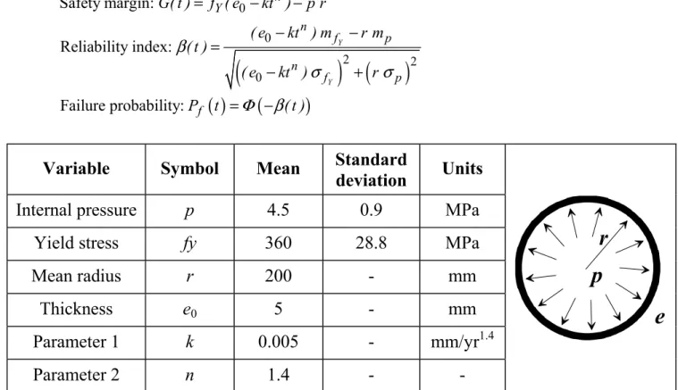
To illustrate some of the above concepts, consider a simple example of a steel pipeline subject to corrosion. The system variables and their distribution parameters are given in Table 14.1 (for simplicity, all the probability distributions are considered as normal). In this example, the tube wall thickness loss is given by the corrosion law of type ktn for t > 1, where t is the time in years, and k and n are the parameters of the corrosion model.

By considering the safety margin corresponding to the material strength regarding hoop stress, the reliability index is found to be 3.904 (the mean of the margin is 4.5 and its standard deviation is 1.153). In the corroded state, the safety margin, the reliability index and the failure probability are given by:

(

)

( )

( ) ( ) 0 0 2 ₂ 0 Safety margin: Reliability index: Failure probability: Y Y n Y n f p n f p f G( t ) f ( e kt ) p r ( e kt ) m r m ( t ) ( e kt ) r P t ( t ) β σ σ Φ β = − − − − = − + = −

Variable Symbol Mean Standard

deviation Units

Internal pressure p 4.5 0.9 MPa

Yield stress fy 360 28.8 MPa

Mean radius r 200 - mm

Thickness e0 5 - mm

Parameter 1 k 0.005 - mm/yr1.4

Parameter 2 n 1.4 - -

Table 14.1. Geometrical and mechanical characteristics of the pipeline

r

e

p

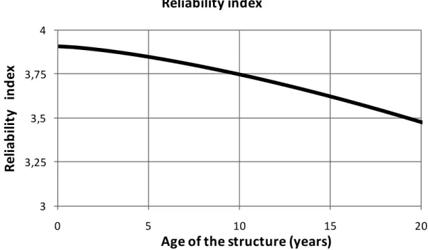
Figure 14.6 depicts the evolution of the reliability index ȕ as a function of the age of the structure t. Table 14.2 indicates various costs involved along the lifetime of the pipe.

Figure 14.6. Reliability index as function of the pipe age

Initial cost of manufacturing and installation _{C0 = 600 k€}

Failure cost _{CF = 30000 k€}

Perfect preventive maintenance cost _{CPM = 20 k€}

Imperfect preventive maintenance cost CIM = 10 k€/mm

Table 14.2. Costs involved during the pipe’s life

In this example, perfect maintenance corresponds to replacement of the pipe by a new one, and imperfect maintenance consists of applying a coating with cost equal to 10 k€ per mm of additional thickness. Without maintenance, the total cost of the pipe is composed of the initial and failure costs. The expected total cost is plotted in Figure 14.7 as a function of the pipe age, where a minimum is observed at 41 years, corresponding to its economic lifetime without maintenance.

3 3,25 3,5 3,75 4 0 5 10 15 20 R el iab il it y in d ex

Age of the structure (years) Reliability index

Figure 14.7. Total cost without maintenance

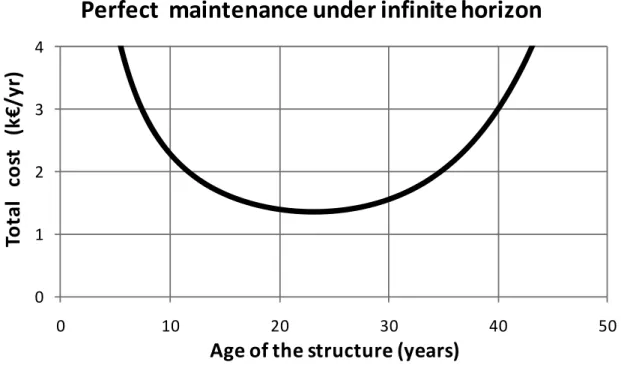
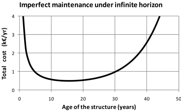
Figures 14.8 and 14.9 depict the costs per unit time in the case of perfect and imperfect maintenance, respectively. In the case of perfect maintenance, optimal maintenance is located at 23 years with a total cost of 1.34 k€/yr. In the case of imperfect maintenance, we have chosen to add 0.3 mm of coating, representing a repair cost of 3 k€. The optimum is located at 16 years with a total cost of 0.49 k€/yr. It is important to note that these values are based on the assumption of an infinite horizon. It can easily be demonstrated that this assumption does not apply in the case of imperfect maintenance, as the maintenance cycles are not identical. In other words, imperfect maintenance is only valid for the first cycle.

Figure 14.8. Perfect maintenance cost according to time interval between operations

0 10 20 30 40 0 10 20 30 40 50 To ta l c o st ( k € /y r)

Age of the structure (years)

Expected cost without maintenance

0 1 2 3 4 0 10 20 30 40 50 To ta l c o st ( k€ /y r)

Age of the structure (years)

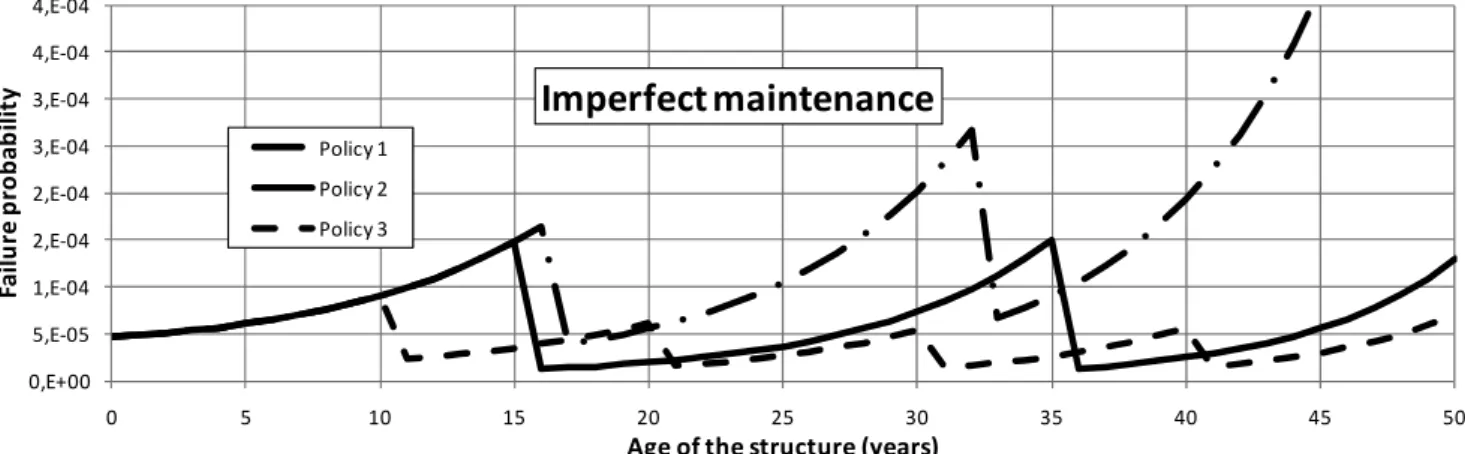
By considering the case of a finite horizon, the curves in Figures 14.10 and 14.11 show the evolution of the failure probabilities associated with different perfect and imperfect maintenance policies, respectively. In this case, we have to calculate the total cost over the service life, which is taken here as 50 years. In the case of perfect maintenance, Table 14.3 indicates various policies and their corresponding costs.

Figure 14.9. Imperfect maintenance cost according to time interval between operations

Perfect maintenance Policy Maintenance

time (years)

Total cost (k€)

Cost per unit time (k€/yr) Remarks One action (infinite horizon) 23 48.9 0.978 Interval obtained

with the assumption of infinite horizon One action

(finite horizon)

25 47.9 0.958 Interval at 50% of the

service life, in order to balance the failure probabilities in the two intervals Two actions 16 and 32 55.7 1.114 Low degradation

levels, but high cost of maintenance

Table 14.3. Maintenance costs in terms of the number of actions and type of horizon

0 1 2 3 4 0 10 20 30 40 50 To ta l c o st ( k€ /y r)

Age of the structure (years)

As the two cycles are supposed to start with a new structure, the failure costs are minimized when the two cycles are identical (i.e. a maintenance operation at 25 years), which explains why the consideration of finite horizon allows us to reduce the total cost. The application of two maintenance actions leads to a significant increase in the maintenance costs, which is not recovered by the benefits of reducing the failure costs.

Figure 14.10. Evolution of the failure probability (perfect maintenance)

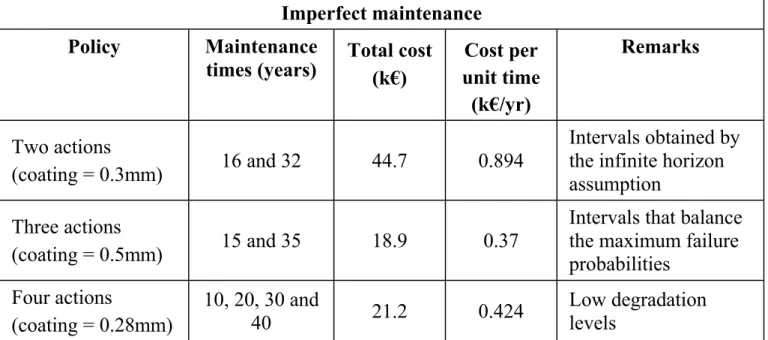
In the case of imperfect maintenance, the assumption of an infinite horizon allows us to optimize the first cycle, but the increase of the failure probability at the end of the lifetime (i.e. at 50 years) leads to very large failure costs. When the maintenance intervals are chosen to balance the failure probabilities by using 0.5 mm of coating, at 15 and 35 years, we obtain a total costs of 18.9 k€ instead of 44 k€. The same strategy is applied with four operations, leading to a higher cost of 21.2 k€.

Imperfect maintenance Policy Maintenance

times (years) Total cost _{(k€) unit time} Cost per (k€/yr)

Remarks

Two actions

(coating = 0.3mm) 16 and 32 44.7 0.894

Intervals obtained by the infinite horizon assumption

Three actions

(coating = 0.5mm) 15 and 35 18.9 0.37

Intervals that balance the maximum failure probabilities

Four actions

(coating = 0.28mm)

10, 20, 30 and

40 21.2 0.424 Low degradation levels

Table 14.4. Maintenance costs in terms of the number of actions and type of horizon

0,E+00 1,E-04 2,E-04 3,E-04 4,E-04 5,E-04 6,E-04 7,E-04 0 5 10 15 20 25 30 35 40 45 50 Fa il u re p ro b a b ilit y

Age of the structure (years) Perfect maintenance

One action (finite horizon) One action (infinite horizon) Two actions

Figure 14.11. Evolution of the failure probability (imperfect maintenance)

14.8. Conclusion

This chapter has introduced several types of reliability-based maintenance models. The main difficulty lies in the estimation of direct and indirect costs of failure, especially when immaterial losses are involved (i.e. human lives, public relations effects, etc.). The formulation of the maintenance cost becomes more difficult when multi-component systems are considered, as economic and stochastic interactions make the analysis very complex. Interested readers can consult the specialized literature, such as [CRE 03], dedicated to the management of infrastructures by considering inspection tool performance, determination of degradation laws, reliability assessment and the choice of maintenance actions.

14.9. Bibliography

[BRE 09] BREYSSE D., ELACHACHI S.M., SHEILS E.,SCHOEFS F., O’CONNOR A., “Life cycle cost analysis of ageing structural components based on non destructive condition assessment”, Australian Journal of Structural Engineering, 9:1, p. 55-66, 2009.

[CRE 03] CREMONA C. (ed.), Application des notions de fiabilité à la gestion des ouvrages

existants, Edition Presses Ponts et Chaussées, Paris, France, 2003.

[FAB 02a] FABER M.H. “RBI: An Introduction”, Structural Engineering International, 3/2002, p. 187-194, 2002.

[FAB 02b] FABER M.H.,SORENSEN J.D., “Indicators for inspection and maintenance planning of concrete structures”, Journal of Structural Safety, 24, 2002.

[GAR 01] GARBATOV Y.,GUEDES SOARES C.,“Cost and reliability based strategies for fatigue maintenance planning of floating structures”, Reliability Engineering and System Safety, 73, p. 293-301, 2001. 0,E+00 5,E-05 1,E-04 2,E-04 2,E-04 3,E-04 3,E-04 4,E-04 4,E-04 0 5 10 15 20 25 30 35 40 45 50 Fa ilu re p ro b ab ilit y

Age of the structure (years)

Imperfect maintenance

Policy 1 Policy 2 Policy 3

[MAD 87] MADSEN H., SKJONG R., TALLIN A. and KIRKEMO F., “Probabilistic fatigue crack growth analysis of offshore structures, with reliability updating through inspection”,

Marine Structural Reliability Symposium, p. 45-55, Arlington, Virginia, USA.

[MOA 97] MOAN T., VÅRDAL O.T., HELLEVIG N.C.,SKJOLDLI, “In-Service Observations of Cracks In North Sea Jackets. A Study on Initial Crack Depth and POD values”,

Proceeding of 16th International Conference on Offshore Mechanics and Arctic Engineering, (O.M.A.E'97), Vol. II Safety and Reliability, p. 189-197, ASME editor,

1997.

[MOA 98] MOAN T., SONG R., “Implication of inspection updating on system fatigue reliability of offshore structures”, Proceeding of the 17th International Conference on

Offshore Mechanics and Arctic Engineering, no. 1214, ASME editor, 1998.

[MOA 99] MOAN T.,JOHANNESEN J.M., VÀRDAL O.T., “Probabilistic inspection planning of jacket structures. In: Offshore Technology Conference Proceedings”, Offshore Technical

Conference, paper no. 10848, Houston, TX, USA, 1999.

[ROU 01] ROUHAN,A., Structural integrity evaluation of existing offshore platforms based on inspection data, PhD, thesis, University of Nantes, France, 2001.

[ROU 03] ROUHAN, A., SCHOEFS, F. “Probabilistic modelling of inspections results for offshore structures”, Structural Safety, 25, p. 379-399, 2003.

[SCH 09] SCHOEFS F., “Risk analysis of structures in presence of stochastic fields of deterioration: coupling of inspection and structural reliability”, Australian Journal of

Structural Engineering, Special Issue - Disaster & Hazard Mitigation, Vol. 9, no. 1, 2009.

[SHE 10] SHEILS E.,O’CONNOR A.,BREYSSE D., SCHOEFS F., YOTTE S., “Development of a two-stage inspection process for the assessment of deteriorating bridge structures”,