Any correspondence concerning this service should be sent to the repository administrator: [email protected]
Official URL:
https://sites.google.com/site/ejaues/home
This is an author-deposited version published in: http://oatao.univ-toulouse.fr/
Eprints ID: 8917
To cite this version:
Attia, El-Awady and Edi, Kouassi Hilaire and Duquenne, Philippe A greedy
heuristic approach for the project scheduling with labour allocation problem.
(2012) In: 12th Al-Azhar Engineering International Conference (AEIC2012),
25-27 Dec 2012 , Cairo, Egypt.
O
pen
A
rchive
T
oulouse
A
rchive
O
uverte (
OATAO
)
OATAO is an open access repository that collects the work of Toulouse researchers and makes it freely available over the web where possible.
1
A GREEDY HEURISTIC APPROACH FOR THE PROJECT
SCHEDULING WITH LABOUR ALLOCATION PROBLEM
El awady ATTIA1, Kouassi Hilaire Edi2, Philippe DUQUENNE1
1 UNIVERSITY OF TOULOUSE/INPT/ ENSIACET/ LGC-UMR-CNRS 5503/PSI/ Industrial Engineering. 4 allée Emile Monso, 31030 Toulouse cedex 4, France. e-mails : {Elawady.attia, Philippe.duquenne}@ensiacet.fr
2 Laboratoire de Mathématique Informatique et Applications, Université Abobo-Adjamé, Abidjan. 21 BP 1288 Abidjan 21. e-mail: [email protected]
Abstract:
Responding to the growing need of generating a robust project scheduling, in this article we present a greedy algorithm to generate the project baseline schedule. The robustness achieved by integrating two dimensions of the human resources flexibilities. The first is the operators’ polyvalence, i.e. each operator has one or more secondary skill(s) beside his principal one, his mastering level being characterized by a factor we call “efficiency”. The second refers to the working time modulation, i.e. the workers have a flexible time-table that may vary on a daily or weekly basis respecting annualized working strategy. Moreover, the activity processing time is a non-increasing function of the number of workforce allocated to create it, also of their heterogynous working efficiencies. This modelling approach has led to a nonlinear optimization model with mixed variables. We present: the problem under study, the greedy algorithm used to solve it, and then results in comparison with those of the genetic algorithms.
Keywords: Robust scheduling, Human resources allocation, temporal flexibility, polyvalence, greedy algorithms.
1 INTRODUCTION
The implementation of an industrial activity requires the analysis and determination of two major entities: first, definition of tasks with their workload moreover to the required skills; the second entity is the workforce with their skills needed to perform these tasks. After the analysis phase, the planner should roughly estimate the work-content, the required resources, and the activities millstones. This stage of planning is known as “macro planning” or the tactical planning level, see, e.g. [1, 2]. After the macro planning, the information becomes available in order to create in some details the operational scheduling that known as the baseline or predictive schedule. But in reasons of the working uncertainty during the execution phase, the orientation is to produce a robust or proactive baseline schedule that is capable to absorb all/some of unforeseen changes. The unexpected events include, but not limited to: unexpected arrival of new orders, cancelling of some orders, shortage of raw material, power shortage, workforce unavailability, machine break-down, accidents at work, over/under estimation of the work-content, etc. As the uncertainty increased as the importance will be to develop firms’ flexibility. This flexibility can be used as a hedge against uncertainty. As defined by [3], the schedule flexibility is the freedom allowed at the execution phase for building the final realized schedule. According to [4, 5], integrating proactive schedules with some built-in flexibility minimises the need of complex search procedures for the reactive algorithm, which also increasing the robustness of the system. Also [4] argued that as the more flexibility in scheduling as the easier to build a robust schedule, moreover, the flexibility indicators can be used to measure the schedule robustness.
Introduced flexibility in scheduling can be done relying on two directions: activities based flexibility, -or resources based flexibility. In activities based flexibility, one can develop the flexibility in activities temporal events, such as the activities start dates. The other dimension is the activities execution sequence; that may have an influence on the start dates also. The activities based flexible schedule can be generated relying on the partial order scheduling as done by [6, 7, 4], or that done by the ordered group assignment [8].
On the other hand, the resources based flexibility refers to the ease of dynamically reallocate one or more resource during the execution phase without disturbing the activities predictive schedule. [9] adopted the general shop problem with integrating: -The multi-resource, -The resource flexibility (a resource may be
2
selected from a given set to create a specified operation with machine dependent processing time), - And the nonlinear routing. Considering the manpower flexibility that we focused on, [10, 11] explored the operational benefits of the job-shop problem by adopting the manpower partial flexibility (cross-trained workers). Recent works in project management [12, 13, 14, 15, 16], in operation management [17, 18] led authors to strongly recommend the developing of multi-functional flexibility in companies workforce. This qualitative dimension of manpower flexibility was stated in the literature with different names such as versatility, multi-skilled, multi-functional, or polyvalence flexibility. It refers to the fact that each operator has one or more secondary skill(s) beside his principal one, his mastering level being characterized by a factor we call “efficiency”. Recently the current authors in [19] investigated some of the factors that can affect this flexibility dimension. On the other side, the temporal flexibility with annualized working time strategy, i.e. the workers have a flexible time-table that may vary on a daily or weekly basis, with respecting legal and modelling millstones. This temporal fluctuation in workforce time-tables provides firms with dynamic working capacities to face the seasonal variations. Many works have been conducted on workforce scheduling with this new flexibility lever (for example, [20, 21, 22, 23, 24].
Answering the increasing need of responsiveness and flexibility for manufacturing companies facing market volatility and uncertainty, the present authors developed a model to characterize the project planning and scheduling problem with workforce allocation in [12, 25]. It refers simultaneously to the two dimensions of the workforce flexibility: The first is the operators’ polyvalence; and the second refers to the working time modulation. This modelling approach has led to a nonlinear optimization model with mixed variables. Therefore, solving it with mathematical programming is tedious due to side constraints, and huge number of variables which produce a combinatorial explosion, so the computational time is extremely increased [26]. Knowing that, the traditional resources constrained project scheduling proposed a great challenge in the arena of operational research due to its NP-hard complexity nature [27, 28, 29 page.34]. This complexity was gradually increased, first by adopting the discrete Time/Cost trade problem, next by considering multi-skilled workforce, [13], and then with the addition of working time constraints [25]. Consequently, the use of these exact methods for solving such problems of industrial size presents a challenge in the arena. We therefore directed towards approximate solutions that can be obtained with heuristic methods. The current authors developed a methodology to solve this problem using genetic algorithm in [25]. Others like [30] developed a “memetic” algorithm for solving only multi-skilled workforce problem with activities pre-defined durations and heterogeneous effectiveness, the algorithm is a hybrid one that combines an evolutionary algorithm (genetic algorithm) and a local search algorithm (for improving). Here, we developed another algorithm to solve this problem rapidly, this greedy algorithm relying mainly on pre-specified priority rules; we called it allocation by priority rules (APR). It consists of presenting the competitive workers, who could handle a given workload, in order to identify the most appropriate one(s). It gives us more interesting results than the genetic algorithm regarding to the pre-defined priorities.
We organized our article as follows: in section 2, we present the model’s mathematical formulation. Sections 3 and 4 introduce an approach to bring a solution: in section 3, a feasibility study will be computed, and section 4 presents the greedy algorithm used to bring a solution. In section 5, an illustration example will be presented. Finally, the conclusions and directions for further research are presented in Section 6.
2 PROBLEM DESCRIPTION
In this paper, we address the project scheduling problem that we introduced in [25]. A project consists of some activities; each one of them contains a set of I unique and original tasks. We only consider one activity (work-package or sub-project) at time. Each task iI requires a given set of competences for its
execution, taken within a group K of all the competences, present in the company. In the other side, our resources are a set A of human resources, each individual or employee (or actor) from these manpower can be able of performing one or more competences from the set K with time dependent performance rate. That is to say, we consider the actors as multi-skilled. Each actor a has a value which indicates his performance for practicing a given competence k, known as his efficiency θa,k . The efficiency θa,k is
3
always between [0,1]; if the actor has an efficiency θa,k = 1, thus this actor can be considered as having a
nominal skill in the competence k. So when this actor is allocated for this skill on a given task, he will perform his job in the standard task’s duration, whereas other actors, whose efficiencies are lower than unity for this skill, will require a longer working time. In this model θa,k [θmin ,1] : θmin represents the
lower limit below which the allocation is not considered as acceptable, for economic and/or quality reasons. While the activity is being processed, competence k of a task i requires a workload Ωi,k, we
assume this workload is well known in advance. For this execution process, if the candidate actor is considered as an expert (θa,k = 1) then the actual competence execution time or the work ωi,k is not
changed, thus ωi,k = Ωi,k . But, in the other case when an actor with (θa,k < 1) is assigned, then the actual
work for this competence workload can be calculated as a function of his efficiency as: ωi,k = Ωi,k / θa,k >
Ωi,k, resulting in an increase of both execution time and labour cost. From this point of view, the actual
execution duration of a task competence di,k is not known in advance and will be considered as a
consequence of the decision about actors’ allocations. Of course there is a relation between the two variables, but this relation is not linear because the skills’ execution process, that may require more than one actor, each actor having his own efficiency. In addition to the multi-skill aspect of the actors, we consider that the company works under a working time modulation strategy. Accordingly, the timetables of its employees may be changed according to the required workloads to be executed. Thus, to balance between the workloads required and the actors’ availability, to respect duration constraints and to minimize execution cost, we must optimize the resources allocation and the competences’ execution periods.
As a result, the problem consists in minimizing a cost function, subject to a set of allocation, scheduling and regulation constraints. First, the objective function is the sum of four cost terms (f1,…f4), as shown in
equation (1). The first term (f1) represents the actual working cost of workforce without overtime, with
standard working hourly cost rate “Ua”. The second term (f2) represents the cost increase due to overtime,
which can be computed by applying a multiplier “u” to the standard hourly rate. The third term (f3)
represents a virtual cost associated to actors’ loss of flexibility at the end of the project, via a virtual cost rate “UFa”: it is a function of the average actors’ occupation rates, relative to the standard weekly
working hours “Cs0”, and it favours the solutions with minimum working hours for the same workload:
this is intended at preserving the future flexibility of the company. The term (f4) charges a penalty cost to
any activity that would finish outside its flexible delivery time window [31]: this cost may result from storage if products are completed too early (useless inventory), or from lateness penalties; it can be calculated with the activity actual duration “LV”, compared to a time window [L – , L + ], defined by
the contractual duration “L” and a tolerance margin . As a result the function (f4) can be written as
equation (1-d). F= f1+ f2+ f3+ f4 (1)
A a S S s as a FW SW U f 1 , 1 (1-a)
A a S S s as a FW SW HS u U f 1 , 2 (1-b)
A a S S s as a S Cs UF f FW SW 1 , 3 /( 0) 1 (1-c)
L LV L L LV L LV L LV UL f f f LV L j if, 0 1 1 ( ) 3 1 4 (1-d)The model constraints:
4
, 1 , , ,
knkaaikj aA, iI, j (2)They ensure that any actor “a” should be assigned for only one competence k, and only on one task i during the working time instance j. The allocation variable a,i,k,j=1 if the actor a is assigned with skill k
on the task i during the working time period j; a,i,k,j=0 otherwise.
- Resources availability constraints: ,
,
, k
i jERik j A
j, kK (3) Constraints (3) insure that, for the set “ρj” of all the tasks under process at the date “j”, the need ofresources ER to perform the workload of the skill “k”, is always lower than or equal to the total staff in this skill (Ak).
- Tasks’ temporal relations constraints:
dSc = dSi +SSi,c, (i ,c) ЄESS (4)
dFc = dSi+ SFi,c, (i ,c) ЄESF (5)
dSc= dFi + FSi,c, (i ,c) ЄEFS (6)
dFc = dFi +FFi,c, (i ,c) ЄEFF (7)
Constraints (4) to (7) denote the constraints of global temporal relations between any (i, c) two tasks’ start dates “dS” and their finish dates “dF”, with a temporal delay, between their events of start (S) or/and
finish (F). For example, the constraints (4) models the synchronisation between “dSi” the start date of task
i to “dSc” the start event of the task c, this synchronisation can be delayed with a lead or lag amount of
time “SSi,c”.
- Skills’ qualitative satisfaction constraints
θmin,k ≤ a,k a,i,k,j ≤ 1, aA, kK, j (8)
The skills’ satisfaction constraints (8) express that the actors cannot be assigned on a given competence without having the minimum level of qualification θmin,k.
- The skill’s quantitative satisfaction constraints , , 1 , , , , , , , , , , k i ER a df dd j aikj aik j ak k i k i k i
iI, kK (9)The workload satisfaction constraints (9) ensure that the total actors’ equivalent working hours for a given competence balance the required workload.
- Tasks duration’s constraints: ,
D d
Dimin i,k imax i, k (10)
Constraints set (10) express that the duration variables di,k must be within the limits of the task’s temporal
window; the task execution time di will be calculated as di = max(di,k) k=1,……to, K.
- Actors’ working time regulation constraints: - For a period of one day:
, 1 1 ,,, ,,, DMaxJ I i K k aikj aikj
a, j (11)5
Where: , , , , , , , k i k i k i j k i a d EE a ERi,k, and
0 , , , , , , min, , ,
j k i a k k a k i and ER a ak k i EE The actors’ maximum number of working hours per day (constraint 11) is always lower than or equal to a pre-specified maximum value of DMaxJ. Considering this, the real workforce ERi,k, available to fulfil the
workload Ωi,k within a period di,k should be defined, representing an equivalent manpower of EEi,k.
- For a period of one week:
, 1 ) 1 ( 1 1 ,,, ,,, ,
NJS s s NJS j I i K k aikj aikj s a aA, sS (12) ωa,s ≤ DMaxS,aA, sS (13)The constraints (12) and (13) express that actors’ working hours per week “ωa,s” is always lower than or
equal to the legal weekly working time “DMaxS”.
- For a reference period of twelve successive weeks:
) ( , , 12 12 1 1 11 , s week A a S DMax p For s s p ap
(14)Equation (14) represents the constraints of actor’s maximum average working hours during a reference working period of 12 successive weeks “DMax12S”; we assumed that the data concerning the actors’ involvements on previous activities have been accurately recorded and are available at any time (this should be included in the data file concerning the company …).
- For a period of one year:
, , a S S s as DSA FW SW
aA (15)The constraints set (15) guarantee that for each actor, his total working hours for the current activity are always lower than his residual yearly working hours, where ωa represents the actor’s working time in the
current year on previous activities, and “DSA” is the maximum annual working hours of any actor.
- Overtime constraints Otherwise 0 , , , DMaxMod if DMaxMod HS as as s a (16) , , a S S s HSas HSA HSR FW SW
aA, (17)Finally the sets (16) and (17) modulate the overtime constraints; overtime hours “HS” can be calculated from equation (16). Accordingly, each actor always has HSa,s [0, DMaxS – DMaxMod] for each
working week “s”, where DMaxMod represents the maximum weekly working time, based on the company internal agreement modulation. Constraints (17) represent the overtime limitations for each actor: from this, an actor’s overtime is always kept lower than or equal to a pre-specified yearly maximum “HAS”. Here we assumed that the actual amount of each actor’s overtime hours “HARa”
performed on other previous activities is available.
3 FEASIBILITY STUDY
Before the generation of the baseline schedule, our general methodology provides a feasibility study, to examine the compatibility between the workload required by activities to be performed, and the capacity assigned to the project during the considered planning horizon. The feasibility study consists in using the maximum flexibility limits, so that if it is impossible to find a satisfactory solution without violating some constraints, it can be pointed out rapidly. Such a validation would stop the procedure before undertaking a long and tedious computing process; moreover it can be used as indicators to allow negotiation for more
6
resources. In the description of the feasibility study and the exploration methodology mentioned above, we will present an illustration example in section 5.
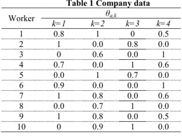
In the present approach, the data necessary to generate the baseline schedule are gathered according to their nature in three different files, as shown in tables (1, 2 and 3): - The file ‘company’ provides all the data concerning the company in charge of performing the activity: mainly the inventory of the actors with their competences, including their respective efficiencies on these competences, table 1. - The file ‘regulation’ gathers the data resulting from the regulation on the working time modulation, table 2. - The file ‘activity’ describes the activity to be carried out, table 3.
From these data, an initial PERT scheduling will be carried out based on the tasks’ standard durations Di,
these durations corresponding to a standard way to proceed in the company. From the result of this initial scheduling, we can calculate: - the initial starting dates of each task dSi, - the activity duration, which will
become by default its fixed contractual duration L, - and the total float of each task fti.
Table 1 Company data Table 2 The regulatory data
Worker θa,k DSA 1600 hours
k=1 k=2 k=3 k=4 HSA 180 hours 1 0.8 1 0 0.5 DMaxS 48 hours 2 1 0.0 0.8 0.0 DMax12S 44 hours 3 0 0.6 0.0 1 DMaxMod 39 hours 4 0.7 0.0 1 0.6 Cs0 35 hours 5 0.0 1 0.7 0.0 DMaxJ 10 hours 6 0.9 0.0 0.0 1 NJS 5 days 7 1 0.8 0.0 0.6 U 11 money unit 8 0.0 0.7 1 0.0 u 0.25 9 1 0.8 0.0 0.5 10 0 0.9 1 0.0
Table 3 Activity data
Task
No. Di Dimin Dimax k=1 k=2 Ωi,k (hours) k=3 k=4 Successors task Relation Delay
1 4 2 6 0 60 0 50 2 – 3 – 4 E-S +0 2 5 3 7 45 68 0 0 3 – 5 – 7 E-S +0 3 4 3 7 0 63 45 35 5 – 6 E-S +0 4 7 5 10 53 0 60 0 6 – 9 E-S +0 5 4 2 6 0 65 0 60 7 – 8 E-S +0 6 3 1 5 60 0 35 0 8 – 9 E-S +0 7 5 3 7 35 56 0 40 10 E-S +0 8 5 3 8 0 0 47 50 10 E-S +0 9 4 2 5 0 45 26 0 10 E-S +0 10 3 2 4 35 30 35 30 -- -- --
The feasibility study is intended to explore the possibility for the company to carry out the activity, taking into account the workforce available to perform it in the considered duration L. More precisely, it makes it possible to highlight the impossibility of the activity execution, without prejudging the actual feasibility. The objective is to eliminate any idea from non-feasibility of the activity by using the maximum limits of the flexibility constraints. This study is processed on two distinct and successive levels: initially, we proceed to a comprehensive study of the availability and the workloads on each competence for the entire duration L; if any conclusion can be emitted with the non-feasibility, we are engaged in a second part with a detailed study.
7
3.1 AGGREGATED ANALYSIS BY COMPETENCE
In the aggregated calculation, we take each competence independently from each other. For each one of them, the available workers are taken into account according to their efficiency, in contrast to the required workload from each skill:
- The maximum equivalent overall capacity of the workers: we understand by this overall capacity, the
equivalent of overall work that can be performed by the workers within the limits of the working time regulation, taking into account their efficiencies. This overall capacity by competence can vary while keeping the workforce of the workers constant. If we call Qk,L the maximum capacity of the workers
having a sufficient efficiency in competence k for the period L, we can define Qk,L as the product of the
maximum duration of weekly work DMaxS by the equivalent workforce of the considered competence
EEk and the number of weeks that we count during the period L; this gives:
1 1 , DMaxS EE LNJS QkL k , k where , min , 1 ,
k a A a ak k EE k (18)In this equation, EEk represent the equivalent workforce of the workers assigned in the competence k
based on their productivities, and NJS the number of working days considered in one week.
- The overall workload by competence: for each task, the workloads Ωi,k are known on all the required
competences. Therefore, we calculate the overall workload by competence wk with the following relation:
, w 1 ,
I i ik k k (19)The project is considered as infeasible and a conclusion of insufficient resources towards the workload will be returned, if we have:
wk ≥ Qk,L, k (20)
In the opposite case, no conclusion can be emitted; we then turn to a more detailed study.
3.2 DAILY ANALYSIS BY COMPETENCE
During this analysis, we use the initial scheduling, which provides for each task: the initial start date dSi
and the total float fti. In order to analyse in some details the compatibility between the workload and the
available capacity of the workforce, we release some constraints of the problem (for the purposes of this test only). We assign to each task the greatest possible duration, which will be the maximum of the following two values: the maximum duration that the activity can take according to its essential data (Dimax), or the period of the standard duration plus the float that previously determined by the initial
scheduling (Di +fti): this duration will then be equal to max(Dimax , Di +fti). This aims to minimize the
daily workloads for each task; as for the preceding study (overall study by competence), it is aimed at highlighting an impossibility of performing the considered activity rather than demonstrating its feasibility. Thus, the inability for the company to cover the workloads as minimized as possible will lead to the conclusion that a research of any further solution is illusory. While assigning to the tasks their maximum durations, we release the precedence constraints for ever in the considered planning horizon (we consider that each task is independent so the initial start dates remain unchanged). Thus the extension of the tasks’ durations defers a part of their workloads on the dates on which their successors are held. That can help to draw the non-compatibility conclusion, between workloads and resources availability during the planning horizon L, of course during the schedule exploration the precedence constraints will obligatorily respected.
- Expression of the maximum daily workload by competence: from the start dates of initial scheduling we
can determine ρk,j, the set of all tasks which are achievable on the day j and mobilizing the competence k.
We make the assumption that the workload Ωi,k of each task is uniformly distributed over its duration (the
duration that we have just fixed at the maximum value that it can take). The global daily workload for a competence is given by the following relation:
k j i i i i k i j k , max( D ,D ft) w max, , , k, j (21)8
After relaxation of the precedence constraints and the attribution of the maximum durations of the tasks, we identify for a day j and for a competence k the workload Ωi,k of tasks which are likely to be realized.
- Expression of the daily maximum availability by competence: during the aggregated calculation, we
determined Qk,L. In the same manner, for each competence, if we call Qk,j , the maximum daily available
capacity, we then have:
L Q Q kL
j
k, , , k (22)
In this relation, we suppose that Qk,j is identical for each day j. In proceeding in this manner, to declare
the activity as non-feasible, it is enough that for a given day j, there is a competence k for which the daily maximum available capacity is lower than the daily maximum workload, that is to say:
k | wk,j ≥ Qk,j , j (23)
As for the global analysis, if this test is verified, we will state the non-feasibility of the activity and stop any search for a solution, to negotiate the resources augmentation. In the opposite case, no conclusion can be emitted at this stage: thus we have to go on solving the problem by exploring solution approach.
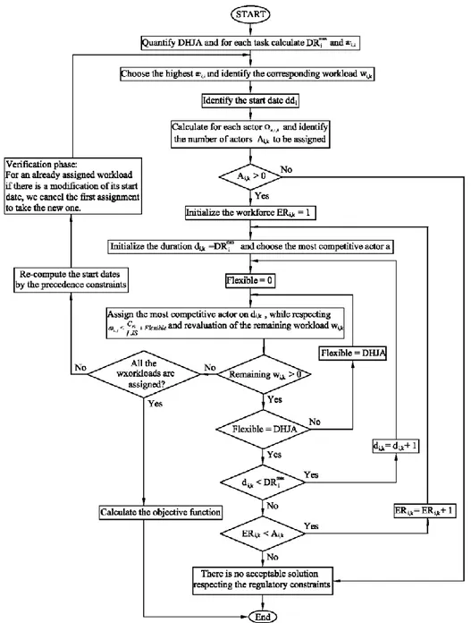
4 THE GREEDY ALGORITHM
The current greedy algorithm is based on the priority rules; we call it allocation by priority rules “APR”. It is a heuristic that is inspired from the same logic of allocation problems with the objectives of: - finding the completion periods of the various tasks, - respecting the calendar targets of the activity, - choosing the best available actors for each task in order to reduce the difference between the workload and the working time, taking into account that the efficiency of some actors may be lower than the nominal value. These objectives imply that the most qualified actors and the most available ones will be privileged for the sake of quality of the outcome. This heuristics will be based on the concept of ‘critical competence’ (Edi, 2007), which will make it possible to index the tasks where the workloads Ωi,k are important and hard to
be executed in the interval of a definite duration [Dimin, DRimax] (where, DRimax = min(Dimax, Di
+ ft
i)
incomparison with the availability of the resources. The principle is to put in competition all the workers likely to be assigned on a workload, and to establish the set of priorities according to which the allocation will be decided.
4.1 CRITICALITY OF COMPETENCE
The criticality τci,k of the workloads Ωi,k on the noted competences allows to prioritize the order of
processing them, knowing that the competences that are the most “charged” (referring to the ratio between workload and available capacity) will be the most ‘rare’, and that it will be advisable to book the corresponding actors as soon as possible. In order to respect the duration interval of task realization and the float obtained in the initial scheduling. Thus, we have:
max , , i k k i k i EE DR c (24)
A given competence will be considered as the more ‘rare’ as τci,k will be higher , - and the sooner its
allocations will have to be treated in the process. And once the treatment sequence of the workloads is established, the choice of the actors will be done by simultaneously taking into account two fundamental criteria: quantitative and qualitative.
4.1.1 Quantitative criterion: intensity of the allocation
The allocation intensity consists in defining the number of actors to be assigned on a task, first of all to balance the workload required upon the expected duration; this problem is then recurring; for a side, the choice of the actors, whose efficiencies may not be nominal, can modify the task duration; on the other side, the same matter of availability can lead the planner to a significant modification of the task duration (within the interval [ min
i
D , max
i
DR ]), which in turn will have an impact on required workforce. Let us note
9
4.1.2 Qualitative criterion: efficiency of human resources
Taking into account the human resources efficiencies in the assignment process, it consists in allocating the most efficient available actors, in order to minimize both the necessary working time (thus the cost), and the impact over the task duration. Because of the availability constraints of the actors, the result may be the assignment of non-optimal resources by using multi-skill concept. The assembly of the two criteria given above makes it possible to establish the rules of priorities that are presented in the next section.
4.2 DESCRIPTION OF THE APPROACH
An actor will be known as ‘competitive’ (i.e. ‘could be assigned’) if the equivalent work “ωa,i,k” that he
must work on the workload Ωi,k is significant compared to that of other actors (knowing that, ωa,i,k
depends on his efficiency θa,k), and if this work can be performed smoothly over the real maximum
duration DRimax. Therefore, the actors whose work can not be evenly spread over the task duration will be
penalized. For every workload Ωi,k to be executed, the equivalent work ωa,i,k for each actor will be
calculated as follows:
min , max , 1 , , ,
k a i i i k a DR dd dd j aj k i a DMaxJ , a, i, k (25)Where, (DmaxJ – Ωa,j) represents the maximum availability of the actor a in the day j and ωa,j represents
his daily global work resulting from all the previous assignments. An “actor penalty” can be applied as follows: for example if (DmaxJ – ωa,j) = 0 for one day j[ddi, (ddi +DRimax–1)], it means that there is no
possibility of assignment of this actor (because he/she reached his/her maximum daily availability), thus we can withdraw (DmaxJθa,k) in the equation of ωa,i,k as a sort of penalty for not to give him/her the
priority (because his work on the workload Ωii,k will not be smooth).
On the basis of this criterion, the group of the actors Ai,k, that can be assigned on the workload will be
prioritized. However, for an actor, it is necessary for him/her to have at least the availability on the period max
i
DR , to have a favourable decision for allocation, i.e.
0 1 , max
i i i DR dd dd j aj DMaxJ , a (26)The maximum daily work of an actor DMaxJ is composed of two durations: a standard duration and a flexible duration. Figure 1 below, shows an example of the distribution of the daily work, within the framework of the modulation of working time regulations in France (where DMaxJ = 10 hours) and in a company where the standard duration of work is fixed at 7 hours.
Figure 1 Distribution of the daily work of an actor
In this methodology, to respect the working time modulation, it is necessary to determine the flexible duration that we can authorize with each actor. We will call DHJA the excess of daily hours allowed for not violating the periodic constraints of the working time. To determine it, we take the most demanding of the regulatory constraints per period; this is calculated over twelve consecutive weeks DMax12S, then we have: NJS C S DMax DHJA 12 s0 (27)
DHJA will be the flexible duration of an actor daily work. According to the adopted regulations (the
French one), this duration will be: DHJA= (44–35)/5=1.8 hours/day, or 9 hours/week. This flexible working time can be regularly used when the seven standard hours are not enough to cover the workload.
10
This average regular temporal flexibility can be used irregularly from working week to other, i.e. it is permissible to increase the weekly working hours for a given worker to 48hours/week, but the average work per a period of 12 weeks should respect the milestone of 44 hours. Knowing that and according to equation 16, the overtime will be computed started from the internal agreement of DMaxMod = 39 hours, this overtime is a very useful but expensive flexibility. Therefore, this flexible duration will be exploited in two stages:
- First, we will use half of this excess, i.e., 1.8/2= 0.9 hours, which will result in an increase of hours per week of 0.95=4.5. Thus a total work of 35+4.5=39.5 hours with overtime of half an hour;
- In the second time, if this excess is still unable to cover the workload, then we use second half that is to say the remaining 4.5 hours with overtime of 5 hours per week.
4.3 CHOICE OF ACTORS AND DETERMINATION OF DURATION
4.4.1 The choice of actors assignment decisions:
a,i,kSetting a competition between actors allows us to choose the best suitable one(s) for performing a workload: they are ranked in order of priority starting from the more competitive according to ωa,i,k.
Therefore the choice will be processed starting with the first actor of the list. From this choice, the real workforces ERi,k is constituted at the same time with the determination of the duration di,k, and thus the
total work that cover the considered workload.
4.4.2 Determination of the durations d
i,kand constitution of workforce ER
i,kConsidering one workload of a task, the determinations of the execution period and of the required workforce, are done simultaneously by incrementing with respecting the lower and maximum limits of each variable; for a workload Ωi,k 0, we must have: Dimin ≤ di,k ≤ DRimax and 1 ≤ ERi,k ≤ Ai,k. Thus, we
begin with setting the real workforce ERi,k value at 1, and the duration di,k at Dimin. If these data do not
cover the workload, then we increment the duration by one day, without affecting the workforce, until it reaches the maximum duration DRimax. If the workload is not always covered with workforce ERi,k =1 and
di,k = DRimax, we increment the workforce by one actor, we re-initialize the duration with his minimal
value, and start again the process until finding a balance which covers the workload. The originality of this procedure is that each time we increment the workforce, the duration is automatically reset at its minimal value di,k = Dimin.
The increment of the duration goes quicker than that of workforce with a simple goal of demanding the lowest possible number of actors, with utilizing the time interval available to us. However, the contrary case can be considered: in a context where the duration would take precedence over the availability of the actors, we could choose to use more actors and to minimize the duration. This case, identical to the previous approach, is not treated here. When an actor is chosen, initial affectation respects daily standard work Cs0/NJS; the flexible part DHJA will be used when the assigned equivalent availability cannot cover
the workload (as illustrated by figure 2).
5 APPLIED NUMERICAL EXAMPLE AND RESULTS
We consider a company where there are K=4 competences and A=10 actors; they are all multi-skilled, each one having one main competence (with an efficiency of θa,k = 1), and additional competences for
which θa,k [θmin,1] (as shown in table 1); in addition, they are working under the working time
regulation shown in table 2; the company must carry out an activity consisting of I=10 tasks for which the data are represented in table 3. In this example, we suppose that all the actors are paid the same hourly rate U (in monetary unit: mu) and that the overtime hours are raised of u=25% compared to the normal hours. The relations between tasks are of the Finish-Start type with zero delays. According to initial
PERT scheduling established with the standards durations Di, the contractual fixed duration is L=25 days,
11
to this contractual duration. To avoid pay lateness penalties, or to support storage cost, it is necessary that the real duration LV lays between: L – ≤ LV ≤L + 20 ≤ LV ≤30 days.
Figure 2 Algorithm of allocation by priority rules: APR
This application example will be used to present our methodology. For presenting it in an easier way, this example is deliberately simple, too much simple to claim to be representative of a real industrial application. However a set of applications of important size is tested and solved with the proposed approach, in conformity with what can be encountered in “the real-world”. In all tested instances the computing rapidity and quality of the solution was proven. For the feasibility study, we will consider two aspects:
- Considering the actors’ multi-skill,
- Case without actors’ multi-skill (in this case, only the principal competence of each actor is considered; all the other additional competences that the actor can acquired are not taken into account).
The methodological approach consists of three inter-dependent parts. Initially, we read the data of the model, starting from data files. Then we enter the feasibility study procedure to investigate the adequacy between the workload and the availability of the company resources; if we find insufficient evidence of the availability to cover the workload (and those in both cases of our study), then we validate the study of
12
non-feasibility of the activity – in other words, we stop looking for a solution, in order to augment the resources. Otherwise we begin the exploration process, as presented above.
5.1 FEASIBILITY STUDY
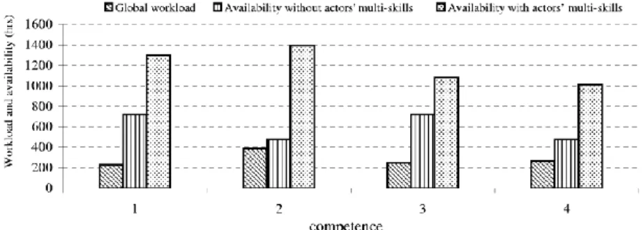
As presented in section 3, the feasibility study is mainly a comparison between the actors’ available capacity and the required workload, either globally for the activity duration or on daily bases. We present in a graphical form (shown in figure 3) the maximum availability Qk,L for each competence in the two
cases (with or without multi-skill), and the global (aggregated) workload wk induced by the activity (these
quantities are expressed in hours). For our example, no conclusion can be emitted with the non-feasibility of the activity, with or without multi-skill; the equivalent overall availability for each competence exceeds the respective aggregated workload. We cannot conclude yet about feasibility, but nothing justifies to stop the calculations at this stage (however, in the case without multi-skills, we note that competence k2 and k4,
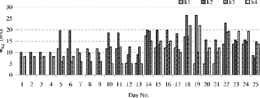
for which we have little difference between the workload and the availability, will certainly cause some concerns). In conclusion, a more detailed study is needed so a daily study for each competence must be conducted. The figure 4, displays the calculation of the actors’ maximum daily availability, and figure 5, provides the maximum daily workload. For reasons of clarity, we separated those two representations. In the case without actors’ multi-skills, no conclusion can be emitted for competences k1 and k3 because their
availabilities (29 hours per day for each one) largely exceed the workload requested. On the other hand, the workloads needed on competences k2 and k4 cannot be assured with the actual availabilities for days
18 and 19 (figure 5).
Figure 3 Aggregated studies by competence
Therefore, without having multi-skilled operators, this application example cannot be carried out by the company. But with multi-skilled actors, the daily workloads for each competence are largely lower than the daily availabilities. Here again, no definitive conclusion can be emitted concerning the feasibility: thus an exploration study is necessary to find the possible solutions.
13
Figure 5 Maximum daily workload by competence
5.2 EXPLORATION WITH APR
This application was tested on a calculator of the type: ‘Intel dual core Xeon 2.4 Ghz with 2.5 GB of Ram’. The coding was carried out on the programming software ‘Visual C++’. The duration of exploration to achieve a workable solution is 1 second (against, from 74 to 155 seconds for the genetic algorithms) as shown in table 4. We present the results in tables and figures allowing a good legibility of the solution. The global durations for each task and those on competences as well as the start dates are represented in table 5. We make the following analysis with task 3: In that table 5, task 3 presents a total duration of execution of: d3 = max(d3,k)k=1 to 4 = 4 days, which respects the duration
constraints( 3) ( 4) ( max 7) 3 3
min
3 d D
D . However, durations of competences (d3,k)k=1 to 4 are all different
but they respect the duration constraint. Thus, actors assigned on the workloads w3,2 and w3,4 work 4 days
while the responsible in charge of w3,3 is released at the end of 3 days. The analysis is the same for the
other tasks. For the precedence constraints, we make the same analysis as follows: table 5, gives the start dates of the tasks. In the ‘activity’ data file, task 3 has for successors, tasks 5 and 8 and as predecessors, task 2. The result provided by table 8 indicates that the start date of task 3 is of dd3= 7 with duration of
d3= 4 days that gives an end of dd3+ d3 = 7+4 =11 days. However the start dates of its successors are: for
task 5 we have (dd5=11) ≥ (dd3+d3=11) and for task 8 we have (dd8=15) ≥ (dd3+d3=11). And for its
predecessor, it is (dd3=11) ≥ (dd2+d2=3+4=7). We notice that the precedence constraints are completely
respected in this case. It is the same for all other tasks. From the data of table 8 we deduce the real duration from execution of the activity LV= max(ddi+di)i=1 to 10 = 22 days . The workforce is represented
too in table 8; we notice that for task 3, the real workforce assigned on the workload w3,2 is of ER3,2=2
actors that represents an equivalent workforce of EE3,2=2 . That means that all the assigned actors have a
nominal efficiency. The global efficiency resulting from this allocation is then:
9450 . 0 60 7 . 56 /10 1 4 1 , 10 1 4 1 ,
i k ik i k ik ER EE opt , and the global work:
10 1 22 1 , 3 . 1173 a j aj hours,
corresponding to a global workload which, of course, has not changed and is still:
10 1 4 1 , 1128 w w i k ik hours.By verifying the daily work of each worker, results indicate to us that no daily constraint has been violated whatever the actor and whatever the day, ωa,j ≤ DMaxJ =10 hours, a,j ; no daily work reaches
9 hours. Also, the summation of work of the actors that we’ve done shows no violation of weekly constraints (like previously, the test was not made over a floating period of twelve consecutive weeks because the real total duration is 22 days). The residual flexibility that represented in equation (27) which records the preserved availability of the actors at the end of the activity is represented by figure 6. Knowing that Oa,s is the worker occupational rate compared to the standard one during the week s, for
more details see, [25].
1
/
1
1
1 / 1 1 ,
NJS
LV
Int
O
FlexR
NJS LV Int s as a
(27)14
Within table 4, we present the different components of performance measures of the proposed heuristic in contrast with genetic algorithms. In the APR, we did not present sub function f5 which represents the
violation of the modulation constraints: indeed, the methodology of the APR does not authorize this violation: f5 can’t have any value but zero.
As a summary the assignment by priorities rules is a heuristics installed to solve in an intelligent way the problem of resources allocation using the concept of competences’ workloads criticality. The capacity of workforce on the workloads and the determination of the tasks durations are done in a simultaneous way until the work of the assigned actors can cover the corresponding workload. Also, the APR is a heuristics which explores the solution set in a reasonable time (1 second in the case of our application example). To demonstrate the effectiveness of either approach, we now will carry out the confrontation of the two results obtained with both methods of exploration.
Table 4 Comparison between results of APR and GA.
Comparison criteria GAs APR
opt
0. 858 0 . 945
Objective function (F) in monetary unit 6 834 . 94 6 316 . 36 Workforce costs without overtime (f1) 14 316. 54 12 816 . 11
Overtime cost (f2) in monetary unit 66 . 68 91 . 69
f3 (storage or lateness penalty cost) 0.00 0.00
f4 (cost of residual flexibility) 7 548.28 6 591.44
F5 : Cost of violation of modulation constraints 0.000 ---
Computing time in second 155 1
Total duration of the activity LV in days 30 22
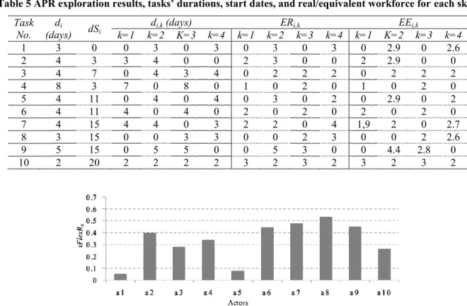
Table 5 APR exploration results, tasks’ durations, start dates, and real/equivalent workforce for each skill. Task
No. (days) dSdi i k=1 k=2 K=3 k=4 k=1 k=2 k=3 k=4 k=1 K=2 k=3 k=4 di,k (days) ERi,k EEi,k
1 3 0 0 3 0 3 0 3 0 3 0 2.9 0 2.6 2 4 3 3 4 0 0 2 3 0 0 2 2.9 0 0 3 4 7 0 4 3 4 0 2 2 2 0 2 2 2 4 8 3 7 0 8 0 1 0 2 0 1 0 2 0 5 4 11 0 4 0 4 0 3 0 2 0 2.9 0 2 6 4 11 4 0 4 0 2 0 2 0 2 0 2 0 7 4 15 4 4 0 3 2 2 0 4 1,9 2 0 2.7 8 3 15 0 0 3 3 0 0 2 3 0 0 2 2.6 9 5 15 0 5 5 0 0 5 3 0 0 4.4 2.8 0 10 2 20 2 2 2 2 3 2 3 2 3 2 3 2
Figure 6 Distribution of average residual flexibility by actor
5.4. THE PROPOSED ALGORITHM VERS GENETIC ALGORITHMS
This paragraph compares our two exploration methods in order to determine which one offers the best results. The comparison criteria that we retained are:
15
- the allocation optimization rate: τopt, to have an idea of the rational use of the actors, - the value of the objective function (F) which represents the overall costs of the activity, - the computing time (duration of exploration),
- the utilization of actors’ multi-skills (which increases the total work thus the cost of working manpower),
- the overtime cost (F2),
- workforce costs without overtime (F1), - real activity total duration LV.
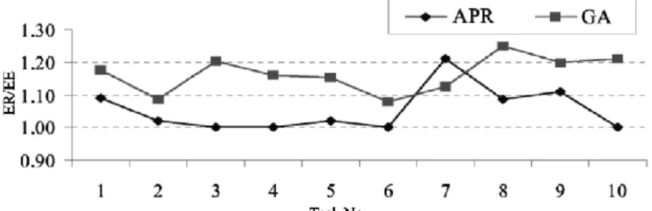
For the criterion of the actors’ multi-skills utilization, we present them on figures 7 and 8. Figure 7, gives the relationship between real to equivalent workforce for each task:
i
EE
ER
EE
ER
K k ik K k ik i i
,
/
1 , 1 , .Indeed, in the company data that provide efficiencies θa,k of each actor, it is clear that each human
resource has a nominal efficiency value for only one competence and non-zero values which are strictly lower than the nominal value in their additional competences. We notice in figure 7 that the allocation made with the APR uses less multi-skill than that of GAs. This logically results from the fact that the APR favours as much as possible the best actors (based one their efficiency, θa,k) to assign them on the
workloads. For example, tasks 3, 4, 6 and 10 have actors’ multi-skills utilization ratio equal to unity: they do not use any additional competence of the actors. On the other hand all the tasks require the multi-skill in the case of exploration with the GAs.
As shown in figure 8, this heavy use of multi-skill flexibility leads to an increase in global work on all competences in the case of GAs, which involves an increase in the workforce costs carried out the workload. On the other hand, with the APR we obtain equality between global work and the total workload on competences 1 and 3 of the company. This result seems odd: competences 2 & 4, that are supposed to be the more critical, should have been affected in priority: thus, the /w ratio should be close to 1 for these competences; a higher value indicates that despite their priority, allocation of less-qualified resources has been necessary to perform the job: it is likely that without multi-skill, this allocation problem would have had no solution. It is also noticed that the curve representing the APR is in all the cases more interesting than that of the GAs.
Figure 7 The ratio between real workforce ER to the equivalent manpower EE
16
Based on these analyses, although both methods produced feasible results without any constraints violation, the exploration with the APR proves to be the most interesting one at all points of view. This is recorded in Table 4, where we note that on all the retained criteria, the APR gives the best result with reduced computing time. Despite the good performances obtained with the two exploration methods, results which enabled us to validate our model, we recognize that the treated example does not reflect industrial reality.
6 CONCLUSIONS
In the article, a greedy heuristic algorithm was presented to generate a robust project baseline schedule, it relying mainly on priority Rules. The solution robustness was achieved based on the integration of some of the workforce flexibility; the workers multi-skilled and the working time modulation with annualised working hours. Furthermore an application example was used to present our methodologies in a detailed form. A comparison between the proposed methodology and genetic algorithms was carried out according to different types of measuring criteria to show the most favourable one. And we found that, the allocation made with the APR “consumes” less multi-skills than that of genetic algorithms – which is quite a logical result since the APR favours as much as possible the best actors to assign them on jobs. And the exploration with the APR proves to be the most interesting, for it provided the best result with a considerably reduced computing time. Despite the good performances obtained with both methods (for they gave feasible solutions without any constraint violation), we must admit that the example presented here does not reflect industrial reality: some more investigation are required to validate our model on a real-life case study. However, the capability of the proposed approaches to solve difficult instances with high number of activities was investigated. One of our perspectives aligned to this work is to develop a rules engine to generate the proactive base line schedule, moreover to dynamically produce the best reactive schedule to changes, if any.
REFERENCES
[ 1] Hans, E.W., Herroelen, W., Leus, R., Wullink, G., “A hierarchical approach to multi-project planning under uncertainty”, Omega, Vol.(35), 2007, pp.563–577.
[ 2] Masmoudi, M., “Tactical and operational project planning under uncertainties: application to helicopter maintenance”, PhD thesis, Toulouse University, France, 2011.
[ 3] Billaut, J.-C., Moukrim, A., Sanlaville, E., “Introduction to Flexibility and Robustness in Scheduling”, in: Billaut, J.-C., Moukrim, A., Sanlaville, E. (Eds.), Flexibility and Robustness in Scheduling. ISTE, 2010, pp.15–33.
[ 4] Herroelen, W., Leus, R., “Project scheduling under uncertainty: Survey and research potentials”, European Journal of Operational Research, Vol.(165), 2005, pp.289–306.
[ 5] Aloulou, M.A., Portmann, M.-C., “An Efficient Proactive-Reactive Scheduling Approach to Hedge Against Shop Floor Disturbances”, in: Kendall, G., Burke, E.K., Petrovic, S., Gendreau, M. (Eds.), Multidisciplinary Scheduling: Theory and Applications. Springer US, 2005, pp. 223–246.
[ 6] Policella, N., Smith, S.F., Cesta, A., Oddi, A., “Generating robust schedules through temporal flexibility”, in: Proceedings of the 14th International Conference on Automated Planning \& Scheduling. Presented at the ICAPS’04, 2004, pp. 209–218.
[ 7] Policella, N., Oddi, A., Smith, S., Cesta, A., “Generating Robust Partial Order Schedules”, in: Wallace, M. (Ed.), Principles and Practice of Constraint Programming – CP 2004, Lecture Notes in Computer Science. Springer Berlin / Heidelberg, 2004, pp. 496–511.
[ 8] Artigues, C., Billaut, J.-C., Esswein, C., “Maximization of solution flexibility for robust shop scheduling”, European Journal of Operational Research, Vol.(165), 2005, 314–328.
[ 9] Dauzère-Pérès, S., Roux, W., Lasserre, J.B., “Multi-resource shop scheduling with resource flexibility”, European Journal of Operational Research, Vol.(107), 1998, pp. 289–305.
[10] Daniels, R.L., Mazzola, J.B., “Flow Shop Scheduling with Resource Flexibility”. Operations Research Vol(42), 1994, pp.504–522.
[11] Daniels, R.L., Mazzola, J.B., Shi, D., “Flow Shop Scheduling with Partial Resource Flexibility”, Management Science, Vol.(50), 2004, pp.658–669.
17
[12] Edi, H.K., “Affectation flexible des ressources dans la planification des activités industrielles: prise en compte de la modulation d’horaires et de la polyvalence”, PhD thesis, Toulouse University, France, 2007.
[13] Bellenguez-Morineau, O., Néron, E., “A Branch-and-Bound method for solving Multi-Skill Project Scheduling Problem”, Operations Research, Vol(41), 2007, pp. 155-170.
[14] Drezet, L., Billaut, J., “A project scheduling problem with labour constraints and time-dependent activities requirements”, International Journal of Production Economics, Vol(112), 2008, pp.217–225. [15] Li, H., Womer, K., “Scheduling projects with multi-skilled personnel by a hybrid MILP/CP benders
decomposition algorithm”, Journal of Scheduling Vol.(12), 2009, pp.281–298.
[16] Valls, V., Perez, A., Quintanilla, S., “Skilled workforce scheduling in Service Centres”, European Journal of Operational Research, Vol.(193), 2009, pp.791–804.
[17] Yang, K.-K., Webster, S., Ruben, R.A., “An evaluation of worker cross training and flexible workdays in job shops”. IIE – Transactions, Vol.(39), 2007, pp.735-746.
[18] Davis, D.J., Kher, H.V., Wagner, B.J., “Influence of workload imbalances on the need for worker flexibility”, Computer & Industrial Engineering, Vol.(57), 2009, pp.319–329.
[19] Attia, E.-A., Dumbrava, V., Duquenne, P., “Factors Affecting the Development of Workforce Versatility”, in: Theodor, B. (Ed.), Information Control Problems in Manufacturing. Presented at the 14th IFAC Symposium on Information Control Problems in Manufacturing, Elsevier, Bucharest, Romania - May 23-25, 2012, pp. 1221–1226.
[20] Hung, R., “Scheduling a workforce under annualized hours”, Int. J. of Production Research, Vol(37), 1999, pp.2419–2427.
[21] Grabot, B., Letouzey, A., “Short-term manpower management in manufacturing systems: new requirements and DSS prototyping”, Computers in Industry, Vol.( 43), 2000, pp.11–29.
[22] Azmat, C., “A case study of single shift planning and scheduling under annualized hours: A simple three-step approach”, European Journal of Operational Research Vol(153), 2004, pp.148–175.
[23] Corominas, A., Pastor, R., “Replanning working time under annualised working hours”, International Journal of Production Research Vol.(48), 2010, pp.1493–1515.
[24] Hertz, A., Lahrichi, N., Widmer, M., “A flexible MILP model for multiple-shift workforce planning under annualized hours”, European Journal of Operational Research, Vol.(200), 2010, pp.860–873. [25] Attia, E.-A., Edi, H.K., Duquenne, P., “Flexible resources allocation techniques: characteristics and
modelling”, Int. J. Operational Research, Vol(14), 2012, pp.221–254.
[26] Oliveira, F., Hamacher, S., Almeida, M.R., “Process industry scheduling optimization using genetic algorithm and mathematical programming” Journal of Intelligent Manufacturing Vol.(22), 2011, pp.801–813.
[27] Neumann, K., Zhan, J., “Heuristics for the minimum project-duration problem with minimal and maximal time lags under fixed resource constraints”, Journal of Intelligent Manufacturing Vol(6), 1995, pp.145–154.
[28] Shue, L.-Y., Zamani, R., “An intelligent search method for project scheduling problems”, Journal of Intelligent Manufacturing, Vol.(10), 1999, pp.279–288.
[29] Brucker, P., Knust, S., “Complex Scheduling”. 2nd ed. Springer Verlag, 2011.
[30] Yannibelli, V., Amandi, A., “A Memetic Approach to Project Scheduling that Maximizes the Effectiveness of the Human Resources Assigned to Project Activities”, in: Corchado, E., Snášel, V., Abraham, A., Wozniak, M., Graña, M., Cho, S.-B. (Eds.), Hybrid Artificial Intelligent Systems, Lecture Notes in Computer Science. Springer Berlin / Heidelberg, 2012, pp. 159–173.
[31] Vidal, E., Duquenne, A., PINGAUD, H., “Optimisation des plans de charge pour un flow-shop dans le cadre d’une production en Juste A Temps: 2- Formulation mathématique”. Presented at the 3ème Congrès Franco-Quebequois de Génie Industriel, Montréal, Québec, Canada, 1999, pp. 1175–1184.