O
pen
A
rchive
T
OULOUSE
A
rchive
O
uverte (
OATAO
)
This is an author-deposited version published in :
http://oatao.univ-toulouse.fr/
Eprints ID : 11386
To link to this article : DOI:10.1109/TSP.2013.2282909
URL :
http://dx.doi.org/10.1109/TSP.2013.2282909
To cite this version : Pascal, Frederic and Bombrun, Lionel and
Tourneret, Jean-Yves and Berthoumieu, Yannick Parameter
estimation for multivariate generalized Gaussian distributions. (2013)
IEEE Transactions on Signal Processing, vol. 61 (n° 23). pp.
5960-5971. ISSN 1053-587X
Any correspondance concerning this service should be sent to the repository
administrator:
staff-oatao@listes-diff.inp-toulouse.fr
OATAO is an open access repository that collects the work of Toulouse researchers and
makes it freely available over the web where possible.
Parameter Estimation For Multivariate
Generalized Gaussian Distributions
Frédéric Pascal, Lionel Bombrun, Member, IEEE, Jean-Yves Tourneret, Senior Member, IEEE, and
Yannick Berthoumieu
Abstract—Due to its heavy-tailed and fully parametric form,
the multivariate generalized Gaussian distribution (MGGD) has been receiving much attention in signal and image processing applications. Considering the estimation issue of the MGGD parameters, the main contribution of this paper is to prove that the maximum likelihood estimator (MLE) of the scatter matrix exists and is unique up to a scalar factor, for a given shape pa-rameter . Moreover, an estimation algorithm based on a Newton-Raphson recursion is proposed for computing the MLE of MGGD parameters. Various experiments conducted on synthetic and real data are presented to illustrate the theoretical derivations in terms of number of iterations and number of samples for different values of the shape parameter. The main conclusion of this work is that the parameters of MGGDs can be estimated using the maximum likelihood principle with good performance.
Index Terms—Covariance matrix estimation, fixed point
algo-rithm, multivariate generalized Gaussian distribution.
I. INTRODUCTION
U
NIVARIATE and multivariate generalized Gaussian distributions (GGDs) have received much attention in the literature. Historically, this family of distributions has been introduced in [1]. Some properties of these distributions have been reported in several papers such as [2]–[4]. These properties include various stochastic representations, simulation methods and probabilistic characteristics. GGDs belong to the family of elliptical distributions (EDs) [5], [6], originally introduced by Kelker in [7] and studied in [8], [9]. Depending on the value of the shape parameter , multivariate GGDs (MGGDs) and the distributions of spherically invariant random vectors share common properties (see [10], [11] for more details).MGGDs have been used intensively in the image processing community. Indeed, including Gaussian and Laplacian distri-butions as special cases, MGGDs are potentially interesting for modeling the statistical properties of various images or features extracted from these images. In particular, the distribution of wavelet or curvelet coefficients has been shown to be modeled
accurately by GGDs [12]–[15]. This property has been exploited for many signal and image processing applications including image denoising [16]–[19], content-based image retrieval [20], [21], image thresholding [22] or texture classification in indus-trial problems [23]. Other applications involving GGDs include radar [24], video coding and denoising [25]–[27] or biomedical signal processing [26], [28], [29]. Finally, it is interesting to note that complex GGDs have been recently studied in [30], [31] and that multivariate regression models with generalized Gaussian errors have been considered in [32].
Considering the important attention devoted to GGDs, esti-mating the parameters of these distributions is clearly an inter-esting issue. Classical estimation methods that have been in-vestigated for univariate GGDs include the maximum likeli-hood (ML) method [33] and the method of moments [34]. In the multivariate context, MGGD parameters can be estimated by a least-squares method as in [18] or by minimizing a distance between the histogram of the observed data and the theoretical probabilities associated with the MGGD [35]. Estimators based on the method of moments and on the ML method have also been proposed in [36]–[38].
Several works have analyzed covariance matrix estimators defined under different modeling assumptions. On the one hand, fixed point (FP) algorithms have been derived and analyzed in [39], [40] for SIRVs. On the other hand, in the context of robust estimation, the properties of M-estimators have been studied by Maronna in [41]. Unfortunately, Maronna’s conditions are not fully satisfied for MGGDs (see remark II.3). This paper shows that despite the non-applicability of Maronna’s results, the MLE of MGGD parameters exists, is unique and can be computed by an FP algorithm. Although the methodology adopted in this paper has some similarities with the one proposed in [39], [40], there are also important differences which require a specific analysis (see for instance remark III.1). More precisely, the FP equation of [39] corresponds to an approximate MLE for SIRVs while in [40] the FP equation results from a different problem (see Eq. (14) in [40] compared to (15) of this paper).
The contributions of this paper are to establish some proper-ties related to the FP equation of the MLE for MGGDs. More precisely, we show that for a given shape parameter belonging to (0, 1), the MLE of the scatter matrix exists and is unique up to a scalar factor.1An iterative algorithm based on a
Newton-Raphson procedure is then proposed to compute the MLE of . The paper is organized as follows. Section II defines the MGGDs considered in this study and derives the MLEs of their parameters. Section III presents the main theoretical results
1From the submission of this paper, another approach based on geodesic
of this paper while a proof outline is given in Section IV. For presentation clarity, full demonstrations are provided in the Appendices. Section V is devoted to simulation results conducted on synthetic and real data. The convergence speed of the proposed estimation algorithm as well as the bias and consistency of the scatter matrix MLE are first investigated using synthetic data. Experimentations performed on real images extracted from the VisTex database are then presented. Conclusions and future works are finally reported in Section VI.
II. PROBLEMFORMULATION
A. Definitions
The probability density function of an MGGD in is defined by [42]
(1)
for any , where is a symmetric real scatter matrix, is the transpose of the vector , and is a so-called density generator defined by
(2)
where is the indicator function on and and are the scale and shape parameters of the MGGD. The matrix will be normalized in this paper according to , where
is the trace of the matrix . It is interesting to note that letting corresponds to the multivariate Gaussian distri-bution. Moreover, when tends toward infinity, the MGGD is known to converge in distribution to a multivariate uniform dis-tribution [42].
B. Stochastic Representation
Let be a random vector of distributed according to an MGGD with scatter matrix and shape parameter . Gómez et al. have shown that admits the following stochastic representation [2]
(3) where means equality in distribution, is a random vector uniformly distributed on the unit sphere of , and is a scalar positive random variable such that
(4) where is the univariate gamma distribution with param-eters and (see [43] for definition).
C. MGGD Parameter Estimation for Known
Let be independent and identically dis-tributed (i.i.d.) random vectors disdis-tributed according to an MGGD with parameters , and . This section studies esti-mators of and based on for a known value
of .2 The MGGD is a particular case of elliptical
distribution that has received much attention in the literature. Following the results of [45] for real elliptical distributions, by differentiating the log-likelihood of vectors with respect to , the MLE of the matrix satisfies the following FP equation
(5)
where . In the particular case of an MGGD with known parameters and , straightforward com-putations lead to
(6)
When the parameter is unknown, the MLEs of and are obtained by differentiating the log-likelihood of
with respect to and yielding
(7)
(8)
After replacing in (6) by its expression (8), the following result can be obtained
(9)
As mentioned before and confirmed by (9), can be estimated independently from the scale parameter . Moreover, the fol-lowing remarks can be made about (9).
Remark II.1: When , (9) is close to the sample
covari-ance matrix (SCM) estimator (the only difference between the SCM estimator and (9) is due to the estimation of the scale pa-rameter that equals 1 for the multivariate Gaussian distribution). For , (9) reduces to the FP covariance matrix estimator studied in [45]–[47].
Remark II.2: Equation (9) remains unchanged if is
re-placed by where is any non-zero real factor. Thus, the solutions of (9) (when there exist) can be determined up to a scale factor . The normalization will be adopted in this paper and will be justified in the simulation section.
Remark II.3: Let us consider the function defined by
(10)
2We note here that most values of encountered in practical applications
belong to the interval (0,1). For instance, is suggested in [44] as a good choice for most images.
where is a positive constant independent of (the index is used here to stress the fact that changes with but does not depend on ). Equation (9) can be rewritten as
(11)
Roughly speaking,3, satisfies Maronna’s conditions
(re-capped below, see [41, p. 53] for more details) for any except the continuity at .
Maronna’s conditions for a function
(i) is non-negative, non increasing, and continuous on .
(ii) Let and . The function
is non decreasing and strictly increasing in the interval
defined by with .
(iii) Let denotes the empirical distribution of . There exists such that for all hy-perplanes with
(12) Because of non continuity of around 0, the properties of M-estimators derived by Maronna cannot be applied directly to the estimators of the MGGD parameters. The objective of Section III is to derive similar properties for the estimator of defined by the FP (9).
D. MGGD Parameter Estimation for Unknown
When the shape parameter of the MGGD is unknown, the MLE of , and is obtained by differentiating the log-likelihood of with respect to and and , i.e., by combining (7) and (8) with the following relation
(13)
where is the digamma function. Equations (9) and (13) show that and can be estimated independently from the scale parameter .
III. STATEMENTS OF THEMAINRESULTS
As the estimation scenario presented in the previous section has some similarities with the FP estimator studied in [39], sim-ilar results about the estimator existence, uniqueness (up to a scale factor) and FP algorithm convergence are expected to be true. This section summarizes the properties of the FP estimator defined by (9) for a known value of (all proofs are provided in the Appendices to simplify the reading). The case of an unknown value of will be discussed in the simulation section.
3Actually, Maronna’s function depends only on the th sample and not on all
the samples as it is the case here!
A. Notations
For any positive integer , denotes the set of integers . For any vector , denotes the Euclidean norm of such as , where is the transpose of . Throughout the paper, we will use several basic results about square matrices, especially regarding the diagonalization of real symmetric and orthogonal matrices. We invite the reader to consult [48] for details about these standard results. Denote as the set of real matrices, the set of orthogonal matrices and the transpose of . The identity matrix of will be denoted as . Several subsets of ma-trices used in the sequel are defined below
• is the subset of defined by the symmetric positive definite matrices;
• is the closure of in , i.e., the subset of defined by the symmetric non negative definite matrices; • For all
(14) where is a compact subset of , being the Frobenius norm.
For , we introduce the open-half line spanned by defined by . Note that the order associated with the cone structure of is called the Loewner order for symmetric matrices of and is defined as follows: for any pair of two symmetric real matrices ,
( respectively) means that the quadratic form defined by is non negative (positive definite respectively), i.e., for all non zero , , ( 0 respectively). Using that order, one has ( respectively) if and only if ( respectively).
This section will make use of the following two applications
(15)
and
(16)
where , and .
The function is the likelihood of in which the parameter has been replaced by its estimator (8), up to a mul-tiplicative constant and a power factor. Indeed
It is clear that is homogeneous of degree zero whereas is homogeneous of degree one, i.e., for all and , one has
In order to understand the relationships between the two func-tions and , we can compute the gradient of at . Straightforward computations lead to
(17) Clearly is an FP of if and only if is a critical point of the vector field defined by on , i.e., .
Remark III.1: There are some close links between the
MGGDs and the SIRV distributions (that are both specific elliptical distributions). However, all MGGDs are not SIRV distributions and conversely. As a consequence, the FP (9) associated with the MGGDs relies on the function which differs from the FP equation studied in [39] (which corresponds to the particular case ) and from that of [40] which corresponds to SIRVs with random multipliers . Similarly, the shape of the function differs significantly from the likelihoods studied in [39] and [40] that are defined as products of integrals depending on the distribution of the unknown multipliers (see [39], [40] for more details).
In the sequel, we also use for to denote the -th iterate of , i.e., , where is repeated times. We also adopt the standard convention , where
is the identity function defined in . To finish this section, we introduce an important assumption about the vectors for • : For any set of indices belonging to and
sat-isfying , the vectors are
linearly independent.
This hypothesis is a key assumption for obtaining all our sub-sequent results. Hypothesis has the following trivial but fundamental consequence that we state as a remark.
Remark III.2: For all vectors with
, , the vector space generated by has dimension .
B. Contributions
The contributions of this paper are summarized in the fol-lowing theorems with proofs outlined in the next section.
Theorem III.1: For a given value of , there exists
with unit norm such that, for all , admits a unique FP of norm equal to . Moreover, reaches its maximum in , the open half-line spanned by
.
Consequently, is the unique positive definite ma-trix of norm one satisfying
(18)
where .
Remark III.3: Theorem III.1 relies on the fact that
reaches its maximum in . In order to prove this result, the function is continuously extended by the zero function on the boundary of , except for the zero matrix. Since is positive and bounded in , we can conclude (see Appendix A for details).
As a consequence of Theorem III.1, the following result can be obtained.
Theorem III.2: Let be the discrete dynamical system
de-fined on by the recursion
(19) Then, for all initial conditions , the resulting sequence
converges to an FP of , i.e., to a point where reaches its maximum.
Theorem III.2 can be used to characterize numerically the points where reaches its maximum and the value of this max-imum. Note that the algorithm defined by (19) does not allow the norm of the FP to be controlled. Therefore, for practical con-venience, a slightly modified algorithm can be used in which a -normalization is applied at each iteration. This modified al-gorithm is proposed in the following corollary
Corollary III.1: The recursion
(20) initialized by
(21) yields a sequence of matrices which converges to the FP up to a scaling factor. Moreover, the matrices
are related to by
IV. PROOFOUTLINE
This section provides the proofs of Theorems III.1 and III.2. Each proof is decomposed into a sequence of lemmas and propositions whose arguments are postponed in the Appendices. For the proofs that can be directly obtained from those of [39], we refer to [39]. In these cases, the differences due to the definitions of the function and the MGGD model for the observed vectors , for , imply only slight modifications.
A. Proof of Theorem III.1
The proof of Theorem III.1 is the consequence of several propositions whose statements are listed below. The first propo-sition shows the existence of an FP satisfying (9).
Proposition IV.1: The supremum of in is finite and is
reached at a point with . Therefore, admits the open-half line as fixed points.
It remains to show that there is no other FP of than those belonging to . For that purpose, it is sufficient to show that all FPs of are collinear. However, Corollary V.1 of [39] indicates that all FPs of are collinear if all the orbits of are bounded in . We recall here that the orbit of associated with is the trajectory of the dynamical system defined in (19) starting at (See [49] for more details about orbits in dynamical systems). Moreover, according to [39], when a function admits an FP, every orbit of is bounded if the following proposition is verified.
Proposition IV.2: The function verifies the following
properties
• (P1): For all , if , then (also true with strict inequalities); • (P2): for all , then
(22) where equality occurs if and only if and are collinear.
Proof: Since the function used in this paper differs from the one used in [39], a specific analysis is required. It is the objective of Appendix B.
To summarize, Proposition IV.1 establishes the existence of matrices satisfying the FP (9) while Proposition IV.2 together with the results of [39] can be used to show that there is a unique matrix of norm 1 satisfying (9).
B. Proof of Theorem III.2
In order to prove Theorem III.2, we have to show that each orbit of converges to an FP of . For that purpose, we con-sider for all the positive limit set associated with , i.e., the set of cluster points of the sequence when
tends to infinity, where and .
Since the orbit of associated with is bounded in , the set is a compact of and is invariant by : for all , . It is clear that the sequence converges if and only if reduces to a single point. According to [39], reduces to a single point if the following proposition is satisfied.
Proposition IV.3: The function is eventually strictly
in-creasing, i.e., for all such that and , then
(23)
Proof: Since the function used in this paper differs from the one used in [39], a specific analysis is required. It is the objective of Appendix C.
V. SIMULATIONS
This section presents simulation results to evaluate the perfor-mance of the MLE for the parameters of MGGDs. The first sce-nario considers i.i.d. dimensional data vectors
distributed according to an MGGD. These vectors have been generated using the stochastic representation (3) with a matrix
defined as
(24)
Fig. 1. Variations of versus number of iterations for ,
and .
In the following, 1000 Monte Carlo runs have been averaged in all experiments to evaluate the performance of the proposed estimation algorithms. Before analyzing the performance of the FP estimators based on (9), we illustrate the importance of the normalization advocated in this paper.
A. Influence of the Normalization
The main advantage of the normalization (i.e., decomposition of as the product , and trace constraint for the matrix ) concerns the convergence speed of the algorithm. To illus-trate this point, Fig. 1 shows the evolution of the criterion
(25)
where for the blue curves and for the red curves. is the Frobenius norm and is the estimator of at step . As observed, the convergence speed is signifi-cantly faster when a normalization condition is imposed at each iteration of the algorithm.
Fig. 2 shows the evolution of the estimated bias and consis-tency of (the plain curves correspond to whereas for the dotted lines) versus the number of samples when is not estimated (the parameters are , and ). The estimated bias of is defined as where the operator is the empirical mean of the estimated matrices
(26)
For a given sample size, the experiments are performed times ( in the following). Note that the bias criterion based on (26) was used in [47] for assessing the performance of matrix estimators. Note also that other approaches based on computing the mean on the manifold of positive definite matrices could also be investigated [50], [51]. The estimated consistency of is verified by computing . As observed, the estimation performance is the same when a normalization constraint for the scatter matrix is imposed or not.
Fig. 2. Influence of the normalization of the scatter matrix on the estimation performance: estimated bias and consistency versus number of samples .
Fig. 3. Variance of versus number of samples .
A similar comment can be made for the shape parameter when this parameter is estimated (see Fig. 3). The Fisher in-formation matrix has been recently derived for the parameters of MGGDs [36]. It has been shown that this matrix only de-pends on the sample size and the shape parameter . The Cramér-Rao lower bounds (CRLBs) for the MGGD parameters can then be obtained by inverting the Fisher information matrix. These CRLBS provide a reference (in terms of variance or mean square error) for any unbiased estimator of the MGGD param-eters. As observed in Fig. 3, the variance of is very close to the Cramér-Rao lower bound for normalized or non-normalized scatter matrices.
To summarize, the normalization of the scatter matrix (de-composition of as the product , and trace constraint for the matrix ) does not affect the statistical properties of the MLE. However, it ensures an increased convergence speed of the algorithm. Note also that a similar normalization was pro-posed in [46, Eq. (15)].
B. Known Shape Parameter
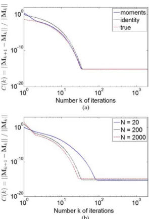
1) Convergence of the Scatter Matrix MLE: Fig. 4 shows
some convergence results associated with the MLE of the scatter
Fig. 4. Variations of for , and . (a) versus number of iterations for different initializations . (b) versus number of iterations for various values of .
matrix . These results have been obtained for ,
(shape parameter) and . Convergence results are first analyzed by evaluating the sequence of criteria defined as
(27) Fig. 4(a) shows examples of criteria obtained for various initial matrices (“moments” stands for equal to the es-timator of moments [36], “identity” stands for and “true” corresponds to ). After about 20 iterations, all curves converge to the same values. Hence, the convergence speed of the proposed algorithm seems to be independent of its initialization. Fig. 4(b) shows the evolution of criteria for various values of . It can be observed that the convergence speed increases with as expected.
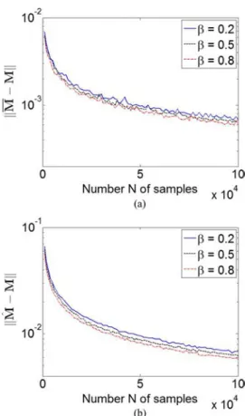
2) Bias and Consistency Analysis: Fig. 5(a) shows the
esti-mated bias of for different values of (precisely for ). As observed, the bias converges very fast to a small value which is independent of . Some consistency re-sults for the proposed estimator are displayed in Fig. 5(b). Here, a plot of as a function of the number of samples is shown for different values of (0.2, 0.5 and 0.8). It can be noticed that, for any value of , converges to a small value when increases.
C. Unknown Shape Parameter
When is unknown, the MLE of and is defined by (9) and (13). If would be known, one might think of using a Newton-Raphson procedure to estimate . The
Fig. 5. (a) Estimated bias for different values of , (b) estimated consistency for different values of .
Newton-Raphson recursion based on (13) is defined by the following recursion
(28)
where is an estimator of at step , and the function has been defined in (13). In practice, when the parameters and are unknown, we propose the following algorithm to es-timate the MGGD parameters.
Algorithm 1: MLE for the parameters of MGGDs 1: Initialization of and .
2: for do
3: Estimation of using one iteration of (9) and normalization.
4: Estimation of by a Newton-Raphson iteration combining (13) and (28).
5: end for
6: Estimation of using (8).
1) Bias and Consistency Analysis: Fig. 6 compares the
al-gorithm performance when the shape parameter is estimated (solid line) and when it is known (dashed line). As observed, the simulation results obtained with the proposed algorithm are very similar to those obtained for a fixed value of .
Fig. 6. Estimated bias and consistency for .
Fig. 7. Estimation performance for parameter . (a) Variance of versus number of samples for , and , (b) Variance of
versus for , and .
2) Shape Parameter : A comparison between the variances
of estimators resulting from the method of moments and the ML principle as well as the corresponding CRLBs are depicted in Fig. 7 (versus the number of samples and versus ). Fig. 7(a) was obtained for , and , while Fig. 7(b)
corresponds to , and . The ML
method yields lower estimation variances compared to the mo-ment-based approach, as expected. Moreover, the CRLB of is very close to the variance of in all cases, illustrating the MLE’s efficiency.
D. Experiments in a Real-World Setting
In this part, we propose to evaluate the performance of the MLE for the parameters of MGGDs encountered in a real-world
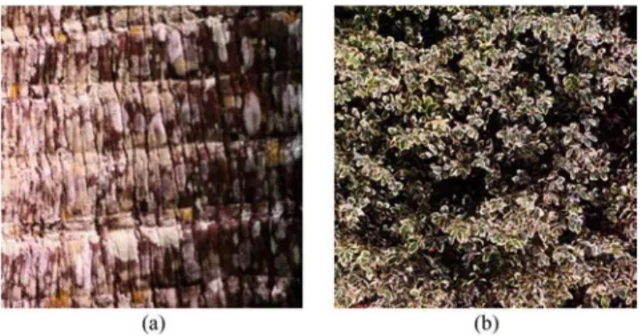
Fig. 8. Images from the VisTex database. (a) Bark.0000 and (b) Leaves.0008. TABLE I
ESTIMATEDMGGD PARAMETERS FOR THEFIRSTSUBBAND OF THEBARK.0000ANDLEAVES.0008 IMAGES
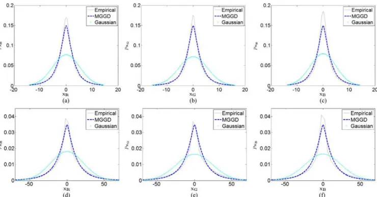
application. MGGDs have been used successfully for modeling the wavelet statistics of texture images [37], [52]. In order to analyze the potential of MGGDs for texture modeling, we have considered two images from the VisTex database [53], namely the “Bark.0000” and “Leaves.0008” images displayed in Fig. 8. The red, green and blue channels of these images have been filtered using the stationary wavelet transform with the Daubechies db4 wavelet. For the first scale and orientation, the observed vector (of size ) contains the realiza-tions of the wavelet coefficients for each channel of the RGB image. MGGD parameters have then been estimated using the proposed MLE for an unknown shape parameter (Algorithm 1), i.e., using the algorithm described in Section V-C. The results are reported in Table I. Fig. 9 compares the marginal distributions of the wavelet coefficients with the estimated MGGD and Gaussian distributions for the first subband of the red, green and blue channels (the top figures correspond to the image “Bark.0000” whereas the bottom figures are for the image “Leaves.0008”). These results illustrate the good potential of MGGDs for modeling color cue dependencies in texture images. For a more in depth analysis, the interested reader is referred to [37], [52] where goodness-of-fit results have been given for wavelet coefficients computed from a large database of natural texture images.
In the next experiments, we have generated 3-dimensional data vectors according to an MGGD with param-eters given in Table I. Fig. 10 shows the MLE performance for these parameters resulting from real texture images. As ob-served in Fig. 10, the performance of the MLE of is very similar when is estimated or not (illustrating the unbiased-ness and consistency properties of the scatter matrix estimator and the MLE efficiency of that have also been observed for synthetic data).
VI. CONCLUSION
This paper has addressed the problem of estimating the parameters of multivariate generalized Gaussian distributions using the maximum likelihood method. For any shape param-eter , we have proved that the maximum likelihood estimator of the scatter matrix exists and is unique up to a scalar factor. By setting to zero the partial derivative with respect to the scale parameter of the likelihood associated with general-ized Gaussian distributions, we obtain a closed form expression of the scale parameter as a function of the scatter matrix. The profile likelihood is then obtained by replacing this expression in the likelihood. The existence of the maximum likelihood estimator of the scatter matrix was proved by showing that this profile likelihood is positive, bounded in the set of symmetric positive definite matrices and equals zero on the boundary of this set. We have also proved that for any initial symmetric positive definite matrix, the sequence of matrices satisfying a fixed point equation converges to the unique maximum of this profile likelihood. Simulations results have illustrated the unbiasedness and consistency properties of the maximum likelihood estimator of the scatter matrix. Surprisingly, these unbiasedness and consistency properties are preserved when the shape parameter of the generalized Gaussian distribution is estimated jointly with the other parameters. Further works include the use of multivariate generalized Gaussian distribu-tions for various remote sensing applicadistribu-tions including change detection, image retrieval and image classification.
APPENDIXA PROOF OFPROPOSITIONIV.1
First, it is interesting to note that if is an FP of , is also an FP of for all . This property is a direct consequence of the homogeneity of degree one of . We start by demonstrating the following lemma.
Lemma A.1: The function can be extended as a
contin-uous function of such that for all non invertible matrix .
Proof: It is enough to show that, for all non invertible
, and all sequence of converging to zero such that is invertible, we have
Using the definition of in (15), the following result can be obtained for all
Since , the conclusion holds true if such that
Fig. 9. Marginal distributions of the wavelet coefficients with the estimated MGGD and Gaussian distributions of the first subband for the red, green and blue channels of the Bark.0000 (a,b,c) and Leaves.0008 images (d,e,f).
End of the Proof of Proposition IV.1: The end of the proof
of Proposition IV.1 is similar to the one given in [39]. Since is defined and continuous in the compact , this function reaches its maximum in at a point denoted as . Since is strictly positive in and equals 0 in , the
inequality leads to . In order to
complete the proof of Proposition IV.1, we need to show the following lemma.
Lemma A.2: Let maximizing the function .
Then, , which implies that is an FP of .
Proof: Since the function defined in (15) differs from
the one used in [39], a specific analysis is required. By definition of , one has
By defining , one has .
The Lagrange theorem ensures that
for . Straightforward computations lead to
Since , one has
which completes the proof of Lemma A.2.
APPENDIXB PROOF OFPROPOSITIONIV.2
We start by establishing . Let with .
Then, and, for all , we have
which proves the property . The reasoning for the case with strict inequalities is identical.
We next turn to the proof of . Using the definition of in (16), the following result can be easily obtained
(B.29)
For all unit vector such that and all , it is well known that
Fig. 10. Estimation performance in a real-world setting. Estimated bias and consistency for (a) the Bark.0000 and (b) the Leaves.0008 settings. Variance of versus number of samples for (c) the Bark.0000 and (d) the Leaves.0008 settings.
where the minimum is reached for the vectors belonging to the line generated by . Moreover, since , one has
For , after noting that the function is un-changed if we replace each vector by the normalized vector
, the following results can be obtained
where
More generally
for all functions and set giving a sense to the previous inequality. The same reasoning can be applied to the function introduced above. Thus, clearly holds true. It re-mains to study when equality occurs in . The property becomes an equality if and only if, for all , one has
(B.31)
which was shown in [39] to be true if and only if and are collinear.
APPENDIXC PROOF OFPROPOSITIONIV.3
The proof of Proposition IV.3 is similar to the proof of Propo-sition V.3 of [39], even if the function used in this paper differs from the one defined in [39]. We first show that for all
, we have
Since implies , for all , we have
Assuming and using hypothesis yields for
all ,
Moreover, assuming that there exists such that
, i.e., implies
which contradicts . Thus,
yields , for all . As a
conse-quence, for all
Since , the previous equality indicates that , for all . Using hypothesis , the claim (C.32) is proved.
We now move to the proof of Proposition IV.3. We consider such that and . As shown above, we
have and , which implies the
existence of an index such that
Note that for , this result reduces to what was obtained in [39]. Up to a relabel, we may assume that , hence
(C.33) which is the same result as the one obtained in [39]. As a conse-quence, the end of the proof of Proposition V.3 derived in [39] can be applied to our problem without any change.
REFERENCES
[1] M. T. Subbotin, “On the law of frequency of error,” Mathematicheskii
Sbornik, vol. 31, no. 2, pp. 296–301, 1923.
[2] E. Gomez, M. A. Gomez-Villegas, and J.-M. Marin, “A multivariate generalization of the power exponential family of distributions,”
Commun. Statist. Theory Methods, vol. 27, no. 3, pp. 589–600, 1998.
[3] E. Gomez, M. A. Gomez-Villegas, and J.-M. Marin, “A matrix variate generalization of the power exponential family of distributions,”
Commun. Statist. Theory Methods, vol. 31, no. 12, pp. 2167–2182,
2002.
[4] K.-S. Song, “A globally convergent and consistent method for esti-mating the shape parameter of a generalized Gaussian distribution,”
IEEE Trans. Inf. Theory, vol. 52, no. 2, pp. 510–527, Feb. 2006.
[5] K. Fang and Y. Zhang, Generalized Multivariate Analysis. Berlin, Germany: Springer, 1990.
[6] K. Fang, S. Kotz, and K. Ng, Symmetric Multivariate and Related
Dis-tributions. New York, NY, USA: Chapman & Hall, 1990.
[7] D. Kelker, “Distribution theory of spherical distributions and a loca-tion-scale parameter generalization,” Sankhyā: The Indian J. Statist.,
Ser. A, vol. 32, no. 4, pp. 419–430, Dec. 1970.
[8] M. Rangaswamy, D. Weiner, and A. Ozturk, “Non-Gaussian random vector identification using spherically invariant random processes,”
IEEE Trans. Aerosp. Electron. Syst., vol. 29, no. 1, pp. 111–124, Jan.
1993.
[9] M. Rangaswamy, D. Weiner, and A. Ozturk, “Computer generation of correlated non-Gaussian radar clutter,” IEEE Trans. Aerosp. Electron.
Syst., vol. 31, no. 1, pp. 106–116, Jan. 1995.
[10] E. Gómez-Sánchez-Manzano, M. Gómez-Villegas, and J. Marín, “Multivariate exponential power distributions as mixtures of normal distributions with Bayesian applications,” Commun. Statist.—Theory
Methods, vol. 37, no. 6, pp. 972–985, 2008.
[11] E. Ollila, D. Tyler, V. Koivunen, and H. Poor, “Complex elliptically symmetric distributions: Survey, new results and applications,” IEEE
Trans. Signal Process., no. 11, pp. 5597–5625, Nov. 2012.
[12] S. G. Mallat, “A theory for multiresolution signal decomposition: The wavelet representation,” IEEE Trans. Patt. Anal. Mach. Intell., vol. 11, no. 7, pp. 674–693, Jul. 1989.
[13] S. Chang, B. Yu, and M. Vetterli, “Adaptive wavelet thresholding for image denoising and compression,” IEEE Trans. Image Process., vol. 9, no. 9, pp. 1522–1531, Sep. 2000.
[14] S. Chang, B. Yu, and M. Vetterli, “Spatially adaptive wavelet thresh-olding with context modeling for image denoising,” IEEE Trans. Image
Process., vol. 9, no. 9, pp. 1532–1546, Sep. 2000.
[15] L. Boubchir and J. Fadili, “Multivariate statistical modeling of images with the curvelet transform,” in Proc. Int. Symp. Signal Process. Its
Appl., Sydney, Australia, Aug. 2005, pp. 747–750.
[16] P. Moulin and J. Liu, “Analysis of multiresolution image denoising schemes using generalized Gaussian and complexity priors,” IEEE
Trans. Inf. Theory, vol. 45, no. 3, pp. 909–919, Apr. 1999.
[17] L. Sendur and I. W. Selesnick, “Bivariate shrinkage functions for wavelet-based denoising exploiting interscale dependency,” IEEE
Trans. Signal Process., vol. 50, no. 11, pp. 2744–2756, Nov. 2002.
[18] D. Cho and T. D. Bui, “Multivariate statistical modeling for image de-noising using wavelet transforms,” Signal Process. Image Commun., vol. 20, no. 1, pp. 77–89, Jan. 2005.
[19] D. Cho, T. D. Bui, and G. Y. Chen, “Image denoising based on wavelet shrinkage using neighbour and level dependency,” Int. J. Wavelets
Multi., vol. 7, no. 3, pp. 299–311, May 2009.
[20] M. Do and M. Vetterli, “Wavelet-based texture retrieval using gener-alized Gaussian density and Kullback-Leibler distance,” IEEE Trans.
Image Process., vol. 11, no. 2, pp. 146–158, Feb. 2002.
[21] G. Verdoolaege, S. D. Backer, and P. Scheunders, “Multiscale colour texture retrieval using the geodesic distance between multivariate gen-eralized Gaussian models,” in Proc. Int. Conf. Image Process (ICIP), San Diego, CA, USA, Oct. 2008, pp. 169–172.
[22] Y. Bazi, L. Bruzzone, and F. Melgani, “Image thresholding based on the EM algorithm and the generalized Gaussian distribution,” Pattern
Recogn., vol. 40, no. 2, pp. 619–634, Feb. 2007.
[23] J. Scharcanski, “A wavelet-based approach for analyzing industrial sto-chastic textures with applications,” IEEE Trans. Syst., Man, Cybern. A,
Syst., Humans, vol. 37, no. 1, pp. 10–22, Jan. 2007.
[24] M. N. Desai and R. S. Mangoubi, “Robust Gaussian and non-Gaussian matched subspace detection,” IEEE Trans. Signal Process., vol. 51, no. 12, pp. 3115–3127, Dec. 2003.
[25] M. Z. Coban and R. M. Mersereau, “Adaptive subband video coding using bivariate generalized Gaussian distribution model,” in Proc.
IEEE ICASSP, Atlanta, GA, USA, May 1996, pp. 1990–1993.
[26] M. Bicego, D. Gonzalo-Jimenez, E. Grosso, and J. L. Alba-Castro, “Generalized Gaussian distributions for sequential data classification,” in Proc. Int. Conf. Pattern Recogn., Tampa, FL, USA, Dec. 2008, pp. 1–4.
[27] J. Yang, Y. Wang, W. Xu, and Q. Dai, “Image and video denoising using adaptive dual-tree discrete wavelet packets,” IEEE Trans.
[28] T. Elguebaly and N. Bouguila, “Bayesian learning of generalized Gaussian mixture models on biomedical images,” in Proc. ANNPR, Cairo, Egypt, Apr. 2010, pp. 207–218.
[29] S. Le Cam, A. Belghith, C. Collet, and F. Salzenstein, “Wheezing sounds detection using multivariate generalized Gaussian distri-butions,” in Proc. IEEE ICASSP, Taipei, Taiwan, Apr. 2009, pp. 541–544.
[30] M. Novey, T. Adali, and A. Roy, “A complex generalized Gaussian dis-tribution—Characterization, generation, and estimation,” IEEE Trans.
Signal Process., vol. 58, no. 3, pp. 1427–1433, Mar. 2010.
[31] M. Novey, T. Adali, and A. Roy, “Circularity and Gaussianity detection using the complex generalized Gaussian distribution,” IEEE Signal
Process. Lett., vol. 16, no. 11, pp. 993–996, Nov. 2009.
[32] M. Liu and H. Bozdogan, “Multivariate regression models with power exponential random errors and subset selection using genetic algorithms with information complexity,” Eur. J. Pure Appl. Math., vol. 1, no. 1, pp. 4–37, 2008.
[33] G. Agro, “Maximum likelihood estimation for the exponential power function parameters,” Commun. Statist.-Simul. Computat., vol. 24, no. 2, pp. 523–536, 1995.
[34] M. K. Varanasi and B. Aazhang, “Parametric generalized Gaussian density estimation,” J. Acoust. Soc. Amer., vol. 86, no. 4, pp. 1404–1415, Oct. 1989.
[35] N. Khelil-Cherif and A. Benazza-Benyahia, “Wavelet-based multi-variate approach for multispectral image indexing,” presented at the SPIE—Conf. Wavelet Appl. Indust. Process., Philadelphia, PA, USA, Oct. 2004.
[36] G. Verdoolaege and P. Scheunders, “On the geometry of multivariate generalized Gaussian models,” J. Math. Imag. Vision, vol. 43, no. 3, pp. 180–193, May 2012.
[37] G. Verdoolaege and P. Scheunders, “Geodesics on the manifold of tivariate generalized Gaussian distributions with an application to mul-ticomponent texture discrimination,” Int. J. Comput. Vis., vol. 95, no. 3, pp. 265–286, May 2011.
[38] T. Zhang, A. Wiesel, and M. Greco, “Multivariate generalized Gaussian distribution: Convexity and graphical models,” IEEE Trans.
Signal Process., vol. 61, no. 16, pp. 4141–4148, 2013.
[39] F. Pascal, Y. Chitour, J. P. Ovarlez, P. Forster, and P. Larzabal, “Covariance structure maximum-likelihood estimates in compound Gaussian noise: Existence and algorithm analysis,” IEEE Trans.
Signal Process., vol. 56, no. 1, pp. 34–48, Jan. 2008.
[40] Y. Chitour and F. Pascal, “Exact maximum likelihood estimates for SIRV covariance matrix: Existence and algorithm analysis,” IEEE
Trans. Signal Process., vol. 56, no. 10, pp. 4563–4573, Oct. 2008.
[41] R. A. Maronna, “Robust M-estimators of multivariate location and scatter,” Ann. Statist., vol. 4, no. 1, pp. 51–67, Jan. 1976.
[42] S. Kotz, “Multivariate distributions at a cross road,” in Statistical
Dis-tributions in Scientific Work, I. Dordrecht, The Netherlands: Reidel, 1968, pp. 247–270.
[43] N. L. Johnson, S. Kotz, and N. Balakrishnan, Continuous Univariate
Distributions. New York, NY, USA: Wiley , 1994.
[44] J. R. Hernandez, M. Amado, and F. Perez-Gonzalez, “DCT-domain watermarking techniques for still images: Detector performance anal-ysis and a new structure,” IEEE Trans. Image Proces., vol. 9, no. 1, pp. 55–68, Jan. 2000.
[45] F. Gini and M. V. Greco, “Covariance matrix estimation for CFAR detection in correlated heavy tailed clutter,” Signal Process., vol. 82, no. 12, pp. 1847–1859, Dec. 2002.
[46] A. Wiesel, “Unified framework to regularized covariance estimation in scaled Gaussian models,” IEEE Trans. Signal Process., vol. 60, no. 1, pp. 29–38, Jan. 2012.
[47] F. Pascal, P. Forster, J. P. Ovarlez, and P. Larzabal, “Performance anal-ysis of covariance matrix estimates in impulsive noise,” IEEE Trans.
Signal Process., vol. 56, no. 6, pp. 2206–2217, Jun. 2008.
[48] R. Horn and C. Johnson, Matrix Analysis. Cambridge, U.K.: Cam-bridge Univ. Press, 1990.
[49] J. Guckenheimer and P. Holmes, Nonlinear Oscillations, Dynamical
Systems, and Bifurcations of Vector Fields. New York, NY, USA: Springer-Verlag, 1983, vol. 42.
[50] S. Sra, “A new metric on the manifold of kernel matrices with appli-cation to matrix geometric means,” in Proc. Adv. Neural Inf. Process.
Syst., 2012, vol. 25, pp. 144–152.
[51] S. Fiori and T. Tanaka, “An algorithm to compute averages on ma-trix Lie groups,” IEEE Trans. Signal Process., vol. 57, no. 12, pp. 4734–4743, Dec. 2009.
[52] R. Kwitt, P. Meerwald, A. Uhl, and G. Verdoolaege, “Testing a mul-tivariate model for wavelet coefficients,” in Proc. Int. Conf. Image
Process. (ICIP), Brussels, Belgium, Sep. 2011, pp. 1301–1304.
[53] MIT Vision and Modeling Group, Vision Texture [Online]. Available: http://vismod.media.mit.edu/pub/VisTex
Frédéric Pascal was born in Sallanches, France in 1979. He received the Master’s degree (“Probabili-ties, Statistics and Applications: Signal, Image and Networks”) with merit, in Applied Statistics from University Paris VII—Jussieu, Paris, France, in 2003. Then, he received the Ph.D. degree of Signal Processing, from University Paris X—Nanterre, advised by Pr. Philippe Forster: “Detection and Estimation in Compound Gaussian Noise” in 2006. This Ph.D. thesis was in collaboration with the French Aerospace Lab (ONERA), Palaiseau, France. From November 2006 to February 2008, he made a post doctoral position in the Signal Processing and Information team of the laboratory SATIE (Système et Applications des Technologies de l’Information et de l’Energie), CNRS, Ecole Normale Supérieure, Cachan, France. From March 2008, he is an Associate Professor in the SONDRA laboratory, SUPELEC. His research interests are estimation in statistical signal processing and radar detection. He is currently on a one-year sabbatical leave in the Electrical and Computer Engineering (ECE) department of the National University of Singapore (NUS).
Lionel Bombrun (S’06–M’09) was born in Tournon, France, in 1982. He received the M.S. and the Ph.D. degrees in signal, image, speech, and telecommuni-cations from the Grenoble National Polytechnic In-stitute (INPG), Grenoble, France, in 2005 and 2008, respectively.
In 2008, he was a Teaching Assistant at Phelma, Grenoble, France. From October 2009 to September 2010, he was a Postdoctoral Fellow from the French National Council for Scientific Research (CNRS) be-tween the Grenoble Image Speech Signal Automatics Laboratory and SONDRA, Gif-sur-Yvette, France. From October 2010 to Au-gust 2011, he was a Postdoctoral Fellow at IMS Bordeaux (UMR 5218). He is currently an Associate Professor at Bordeaux Sciences Agro and a member of the IMS laboratory. His research interests include image processing, stochastic modeling, and texture analysis.
Jean-Yves Tourneret (SM’08) received the in-génieur degree in electrical engineering from the Ecole Nationale Supérieure d’Electronique, d’Elec-trotechnique, d’Informatique, d’Hydraulique et des Télécommunications (ENSEEIHT) de Toulouse in 1989 and the Ph.D. degree from the National Polytechnic Institute, Toulouse, in 1992.
He is currently a Professor with the University of Toulouse (ENSEEIHT) and a member of the IRIT laboratory (UMR 5505 of the CNRS). His research activities are centered around statistical signal and image processing with a particular interest to Bayesian and Markov chain Monte Carlo (MCMC) methods.
Dr. Tourneret has been involved in the organization of several conferences in-cluding the European conference on signal processing EUSIPCO’02 (Program Chair), the International Conference ICASSP’06 (plenaries), the Statistical Signal Processing Workshop SSP’12 (international liaisons), the International Workshop on Computational Advances in Multi-Sensor Adaptive Processing CAMSAP 2013 (local arrangement), and the Statistical Signal Processing Workshop SSP’2014 (special sessions). He has been the General Chair of the CIMI Workshop on Optimization and Statistics in Image Processing, Toulouse, in 2013. He has been a member of different technical committees including the Signal Processing Theory and Methods (SPTM) committee of the IEEE Signal Processing Society (2001–2007, 2010–present). He has been serving as an Associate Editor for the IEEE TRANSACTIONS ONSIGNALPROCESSING
(2008–2011) and for the EURASIP Journal on Signal Processing (since July 2013).
Yannick Berthoumieu received the Ph.D. degree in January 1996 in signal processing from the Univer-sity of Bordeaux I, France.
In 1998, he joined the Ecole Nationale Supérieure d’Electronique, Informatique et Radiocommuni-cations de Bordeaux as an Assistant Professor. He is currently a Professor with the Department of Telecommunications, Poly-technique Institute of Bordeaux, and the University of Bordeaux. His major research interests are concerned with multi-dimensional signal analysis, stochastic modeling, texture analysis, and video processing. Since 2003, he has been with the Signal and Image Processing Research Group, IMS Lab.