Decision support with ill-known criteria in the collaborative supply chain context
12
0
0
Texte intégral
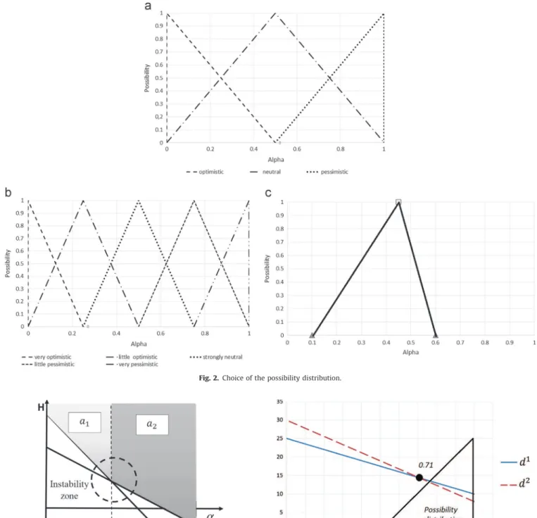
Figure
Documents relatifs
In the literature, different kind of decisions models (short term and long term) treated and considered by many authors separately. For example, different facility location decision
