ESSAIS EN ÉCONOMIE MONÉTAIRE
THÈSE
PRÉSENTÉE
COi\li\lE EXIGENCE PARTIELLE
DU DOCTORAT EN ÉCONOi\lIQUE
PAR
NILOUFAR E\'TEl\HABI
ESSAYS IN MONETARY ECONOMICS
THESIS
PRESENTED
IN
PARTIAL FULLFILMENT
OF THE REQUIREMENTS
FOR THE DEGREE OF
DOCTOR OF PHILOSOPHY IN ECONOMICS
BY
NILOUF AR ENTEKHABI
Avertissement
La diffusion de cette thèse se fait dans le respect des droits de son auteur, qui a signé le
formulaire Autorisation de reproduire et de diffuser un travail de recherche de cycles
supérieurs (SDU-522 - Rév.01-200G). Cette autorisation stipule que «conformément
à
l'article 11 du Règlement no 8 des études de cycles supérieurs, [l'auteur] concède
à
l'Université du Québec
à
Montréal une licence non exclusive d'utilisation et de
publication de la totalité ou d'une partie importante de [son] travail de recherche pour
des fins pédagogiques et non commerciales.
Plus précisément, [l'auteur] autorise
l'Université du Québec
à Montréal
à
reproduire, diffuser, prêter, distribuer ou vendre des
copies de [son] travail de recherche
à
des fins non commerciales sur quelque support
que ce soit, y compris l'Internet. Cette licence et cette autorisation n'entraînent pas une
renonciation de [la] part [de l'auteur] à [ses] droits moraux ni à [ses] droits de propriété
intellectuelle. Sauf entente contraire, [l'auteur] conserve la liberté de diffuser et de
commercialiser ou non ce travail dont [il] possède un exemplaire.»
l ,1m forever indebted t.o m)' ndvisor. Steve Ambler. for his ad vice. inspirnt.ian, guid3nce, availabilit.y, and last bllt Ilot least his finanrial support.
l express my gratitude ta the thesis COIIlInittee: Al3in Guay. André Kurmann, and Hafedh Bouakez for their review of t.he thesis and t.heir const.ruct.in' feeclbark.
l sincerely thank ail our stnff nt the department of Economies and the Ccnt.re Int.eruni\'ersitaire sur le Risque. les Politiques Économiques et l'Emploi (CIRPÉE) for their unfailing caoperMion with stuclents. Special t.hanks to Jérémy Chauclournc for being availnble to h3n<lle the 13st· minute technical issues.
l am thankful for t.he discussions and the valuable suggestions l received during my stay at the University of 1\linnesotn (2004) and my internship nt the International 1\lonetary Fund (2005). l speciill1.l· thnnk AlIbhik Khan. Behzad Diba and Hossein Samiei. Louis Phell1euf is also 3ckllowledged for the scholnrship he offer0d me in 2006.
<lm grateful to my professors. to thosc who gave l'ne the passion for cOlldllct. ing resean:h. l am nlso indebted to 111.1' studellts whose curiosity dC0pelH'c1 ln.Y 0\\'11
understanding of J)1nny complcx ('conomie issues.
Speci,d thanks to my deell' mOIll Il'hose stays during t.l1(' hard times of this thcsis in Cnnnda provided me with the' 1)(>'1('<' of Illilld to studv. Nader. :'-largues. Fnrimah. Abbas. Yalda. 1<al'eh. Dnra. Fati: Pnri. Soravn. \1<1na. 011'<1. Nicolas ,1lld "II otl10r lo\'ed ones <lre gr<lt.efully th,)J)ked.
Finall.\'. thanks to Fréciérie for his cOlltilluing ellcouulgernenL support ancllovc.
LIST OF FIGURES
viii
LIST OF TABLES
xABSTRACT
xiii
RÉSUMÉ ..
xv
INTRODUCTION
1
CHAPTER
l
CLOSE-EMBRACE: CANADA-US COMMON TRENDS
71.1
Introduction.
7
1.2 The Model
101.2.1
The Representative Household
11
1.2.2 The Government
13
1.2.3
The Representative Firm
13
1.2.4
National Accounting .
15
1.2.5
The First Order Conditions
15
1.2.6
Equilibrium Conditions
16
1.3 Econometrie Method .
18
1. 3.1
Identification
19
1.4 Empirical Analysis
21
1.4.1
Data . . . .
22
1.4.2
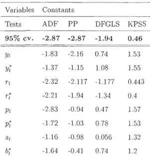
Unit Root Tests
22
1.4.3
Cointegration Tests
23
1.4.4 Estimation and Testing of the Model .
23
1.4.5
Permanent. Shocks or Cornmon Trends .
26
1.5 Conclusions
30
APPENDIX A
APPENDIX B
EQUILIBRIUM CONDITIONS
37
B.1 Fil'st Order Conditions . . .
37
B.2 Derivation of Long-l'un Relations
39
APPENDIX C
FIGURES
42
CHAPTER II
TECHNICAL CHANGE, WAGE AND PRICE DISPERSION, AND THE OPTI
MAL RATE OF INFLATION
47
2.1
Introduction.
47
2.2 The Model
52
2.2.1
Households: Intermediate Labor Market
53
2.2.2
Labor Broker
54
2.2.3
Technology
56
2.2.4
Intel'mediate Goods Firms .
56
2.2.5
Final Goods Firm
58
2.2.6
Monetary Policy
59
2.2.7
Equilibrium .
61
2.3 Steady-State Analysis
62
2.3.1
Steady-State Distortions.
62
2.3.2
Calibration
65
2.3.3
Results
. .66
2.3.4
Steady-State Welfare .
68
2.3.5
Sensitivity Analysis
70
2.4 Dynamic Economy
71
2.4.1
Results
71
2.5
Conclusion
72
APPENDIX A
TABLES . . . .
75
APPENDIX B
EQUILIBRIUM CONDITIONS
79
B.1 The First Order Conditions of Households:
B.2 Key Equations
.
B.3 Steady-State Derivations.
APPENDIX C
FIGURES
CHAPTER III
TO FIX OR TO FLOAT? A THEORETICAL ASSESSMENT
3.1
Introduction.
3.2 Model Economy
3.2.1
Households
3.2.2
International Financial Markets.
3.2.3
Goods Market
3.2.4
Monetary Policy
3.2.5
Government .
3.2.6
Current Account
3.2.7
Shocks .
3.3 Calibration and Simulation
3.3.1
Calibration
3.3.2
Simulation
3.4 Results
.
3.4.1
Steady-State Analysis
3.4.2
Baseline Model . . . .
3.4.3
Impulse Response Analysis
3.4.4
Welfare Analysis ..
3.4.5
Sensitivity Analysis
3.5 Conclusion
APPENDIX A
TABLES . . . .
APPENDIX B
EQUILIBRIUM CONDITIONS
B.1 First Order Conditions . . .
79
80
81
83
88
88
92
94
96
97
97
98
98
99
99
99
101
101
102
102
103
105
106
108
110
118 118B. 2 The System of Equations .
118B.3 Deterministic Steady-State
120
APPENDIX C
FIGURES
123
CONCLUSION .
127
BIBLIOGRAPHY
131
1.1 Impulse response fUllction of one percent deviat.ion shock t,o foreign in terest rat.e ou out,put. . . . . . 42
1.2 Impulse response funct.ion of one percent. c!eviat.ioll shock to foreign in-t.erest rat.e on interest rat.e
1.3 Impulse response function of one percent deviat,ion shock to foreign out put on prices , . . . .. 43
1.4 Impulse response function of one percent cJeviMion shoc:k to foreign Ollt
put, on int.erest rate . . . . 44
1.5 Impulse responsc function or one percent deviat.ion shock to foreigu out put on exch<1nge rate. . . . .. 44
1.6 Impulse response function of one percent. deviiltion shoek to foreign out
put. on output ..
45
1.7 Impulse responsc fllnetion of one percent deviation shock to exchange
rat.e on net accumulation of ilsset·s ..
45
1.8 Impulse respollse funetiou of one percent cJeviHtion shock to rxch<1u?;e
l'Rte on output 46
1.9 Impulse response fllnet iOIl of one percent. cJeviation shock to excil<lnge
rate on interest, l'Rte ..
4G
2.2 Model (ii): 0.5% quarterly growth, and different values for elastieit.y in
the labor and goods markets . . . . . . . . 84
2.3 Priees and wages mark-up distortions 85
2.4 One percent eont.raetionary monetary polie)' shock, Taylor rule with priee
and wage inflations, output growth and smoothing effeet 86
2.5 One percent positive out.put growtlJ ::;hocJ( .
87
3.1 One percent positive real shock in a fixed regirne, when NT stands fol'
Non-t.raders, and T stands for Traders . . . . . . .. 123
3.2 One percent positive monetary shock in il fixed regime 124
3.3 One percent positivE' rE'al shoek in a flexible regime .. 125
1.1 List, of Variables and their Descript ions 31
1.2 Unit. Root. Tests. ;32
1.3 Unit Root. Test.s . 33
1.4 Coint.egrat.ion Rank Tests
34
1.5 Residual- Based Test of the N ull of Coint.egrat.ion Against the Alterna tive
of No Coint.egration . . . . . . . . 34
1.6 VAR Lag Length Selection Criteria
1.7 Test, of \Veak Exogeneit.y . ;15
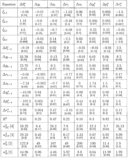
1.8 Errol' Correction Specificat.ion of the i\lodel EconolllY 36
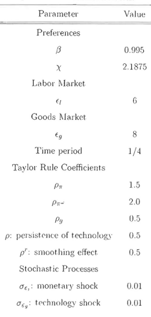
2.1 i\lodeJ Calibration . 7:')
2.2 Sensitivit.y Ana!ysis of Steildy-State Welfarc t.o Stemly-StMe Quarterly
1nfhtion . . . . . . 76
2.3 Scnsitivity AnaJysis or PrieE' I\ larkup Distortion to Stcaclv-State Qu<)[' terJy Inftat ion . . . . . . . . , . . . . . . . . . 7(j
2.4 Sensitivity Ancdysis of Wage l\larkup Distort,iol1 to Steady-State QUM'
ter!y Inflation 76
2.5 Stochastic i\leans basecl on Quarterly Calibration in i\lodeJ (i) , 7G
2.7 Stochastic r.Jeans based on Quarterly Calibration in IVlodel (ii) 77
2.8 St.ochastic Means based on Quarterly Calibration in Model (ii)
78
2.9 Stochastic T\leans based on Quarterly Calibration in Model (ii)
78
3.1 Model Cédibrat.ion . 110
3.2 Steady-StMe VaIlles 111
3.3 Second Moment.s for Symmet.ric Shocks in Baseline Model 112
3.4 Periocl U tilities for Symmet.ric Shocks in BnsclinC' i\Iodcl 112
3.5 \Velfi1reE\1\luilt.ion for Symmet.ric Shocks in Baselinc Model 112
3.6 Business Cycles in the Baseline T\'1odel . . . 113
3.7 Second i\Ioments for Asymmetric Shocks; Dominnncc of i\Ionetary Shock 113
3.8 Period Ut.ilities, Domincmce of rvlonet.ary Shock .. 114
3.9 \iVelfClre Evaluntion. Dominance of Monet.ary Shock 114
3.10 Second i\loment.s for Asymmetric Shocks; Dominimc:e of Real Shock 114
3.11 Periocl Ut.ilities. Dominance of Reni Shock . . . 115
3.12 VVelfClre EH,luCltion, Dominance of Real Shock . 115
3.13 Period U tilit ies. SYll1rnetric Shocks wit h Different Share of NOIl-traders
l'rom Tot,,1 PO]J\lliltion . . . . . . . . ]15
3.14 Period Ut.ilities. Dominance of i\lonetnry Shock with Diff'<:'rent Share of
Non-trndC'rs l'rom Total Populnt.ion . . . 116
3.1S Periocl UtiJities. Dominance of Real Shock \\·it.]} Different SharC' of Non
3.16 Periocl Utilities, Symmetric Shocks with Different Share of Non-traders from Total Population . . . . . 116
3.17 Period Utilit.ies, Dominance of Monetary Shock \Vith Different. Share of
Non-traders from Tot.al Population . . . . . 117
:3.18 Period U tilit.ies, Domini\.nce of Real Shock Dominance with Different
This thesis consists of three essays in monetary economics in general equiJibrium models. Each deals wit.h a probJem that cent.ral banks commonly face: uncertninty, inflation stability, and exchange rate policy.
The first. essay examines t.he interdepenclence of the Canaclian nnd
US
economies with a view t.o common policy allalysis. The est.imatecl struct.ural vector error correc tion model applied to post.-war dat.n confirms t.he presence of four long-run equilibriurn rclationships between the t.wo economies: i) purchasing power parit.y, ii) technological dependence, iii) interest rate parit.y, and iv) net. foreign assets accumulation. Four com mon trenels are also ielentifieel between the two economies: i) technologicaL ii) interest rate, iii) priee, and iv) exchange l'Me relations. The rcsults highJight that exchange rat.e appreciation is consistent with the decrease in foreign assets in Canaclél, that Canada andUS
cycles arc correlHted. that monetary shocks have short-l'un effects on out.puts and permanent effects on pricp levels <Illd pxchange rates in both countries, and thnt t.J1P long-l'un growt.h for bot.h cconomies stems from technologicill innovat.ions. Therefore any expansionary monetnry po\icics in these t.\Vo count.rics should be trcatcc! cautiously as they might leael to inflM.ion in both cconOlllies.The second essi'lY derivE's the opt.imel! rate of priee inflation by adding the clement of long-run growt.h t.o i'I st.anelarel Ne\\' KeYllesian model with both price and wage
rigidities. The resu\ts revive the o leI paradigm of monet.ary economics associated \Vith Frieell1li'ln (1969): milel deflation is the optimal policy. HoweveL in this environment, optimi'll defl(ltion results from growt II. The presence of l'cal gro\Vth in the stcady-state If'ads to a wedge between priee inflation i'lnd wage inflation. In this environl1lenL the st.ei1dy-stnt.e of t.he model is dlill(lcterizecl by four distortions: price dispersion. \Vi1gc c1ispPl'sion, <'lI1d monopoJistic mark-ups of priee a.nd of wage setters Opt.imi:\l infli:ltion is t.he one thM balances these distortions (lt t.be l11i:1l'gin. The welfare gilin of moving fl'Orn zel'O infli:1tion to optimal ckflation is 0.1 o/c: of the steady-state consumption. The c:ost of infléltion in th is environrnent tUl'l1S ou t to be higlJer thi:ln thilt in a mode! \\'it hout gl'Owtlt. This highlights the contribution of growth to the (Ost of inflation. In a stoc:bnstie \'crsion of t he mode!' the mean of \(1l'iables is ilft'ected by SllOCks. As groll'lll tn'(Ilt~s el gèlp bet\reen \vage i1nel priee inflations. the monetary policy ((111 stilbilize \Vilges wh en
tilrgeting a small priee c1eflHtion rate.
The thinl eSSilV addresses the issue of opt.il1wl cxchange rate reginws for (·'m<?rging ceonomies. Il tloes so t hrough t hf' de\'e[opl11ent of n small open econ0l11Y mode! of ('nclo\\'111enl \Vith nOll1ini'll HcxibiJitv i1THI l'Cil 1 rigiclity, i.E'. int'Cl'l1eltional financ:inl In(\1'J«-'t
has important. implicat.ions for t.he choice of ex ch ange regime in these economies. The simulation exercises reveal that. agents who are excluded from t.he foreign exchange market (non-t.raders) marginally prefer flexible exchange rates, while t.hose who have aceess to t.he foreign exchange market (traders) are better off with fixed rates. Flexible rat.es yield a potent.ial Pareto improvement if t.ra.ders represent a very small fraction of the tot.al population. Plausible \veight.s on the two groups in a ut.iJitarian social welfare function give a higher level of social welfare under fixed rates. These results have import.ant implicat.ions for policymakers in emerging markets. An optimal monetary policy, in order to increase t.he average level of welfare. t·urns out t.o be distort.ionary t.owards t.he consumption of non-traders.
Key words: Vector error correct.ion modeL identification, struct.ural shocks, com mon trends, priee inflat.ion, wage inflation, growt.h, staggered cont.racts, welfare evalua tion, monet.ary policy, inftat.ion t.argeting, exchange rate regimes.
Cette thèse est composée de t.rois essais sur l'économie monétaire à lïntérieur du modèle d'équilibre général. Chacun tr(lite d'un problème auquel les bmlques centmles font. souvent· face: l'incert.it.ude, l'iuflat.ion, et. les régimes de t.aux de change.
Le premier essai examine l'interdépendance des économies canadienne et. américaine afin de dégager une analyse des politiques économiques conjoncturelles. Le moclèJe struc t.urel vectoriel des corrections d'erreurs appliqué aux données de l'après-guerre confirme la présence de quatre relations de long terme entre ces deux économies i) la parité du pouvoir d'achélt, ii) la dépendance technologique. iii) la parit.é des taux d'intérêts, et iv) 1'accumulat,ion net.t.e d'actifs ét.r(lngers au Canada. Qu<1t..re tendances communes sont également. identifiées entre les deux économies: i) technologique. (ii) de tnux d'intérêt. (iii) cie prix. et iv) de relat.ion de tnux de ch(lnge. Les résultats suggèrent (jlle
l'appréciation du tnux de chnnge est. conforme à la baisse des actifs (lU Canada, que les cycles cles États-Unis et. du C<'lnada sont corrélés. que les chocs monétaires ont des effets de court terme sur les productions et des effets pcrl1l(lnent..s Sllr les niveaux de prix et· de taux de change dans les deux pays. et que la croissance de long terme des deux pays découle cie l'innovat.ion technologique. Il en résulte que toute politique monétaire expansionnist.e dans ces deux pays doit être gérée avec prudence car el Je pourrait mener
n
de l'inflat.ion.Le second essai dérive Je taux d'inflation optimal des prix en i'\joutant un élémelJt de croissi'\nce de long terme non nulle à un modèle néo-keynesien avec rigidité cie prix et de salaire. Les résultat.s raniment. le vieux pflradigme d'économie monétaire nssocié à Friedman (1969) : une politique légèrement défiéltionnist.e est optimale. Néartlnoins, ce résultat n'est pas dû à l'aspect. monét.aire du mod~~le, mi'\is plut.ôt à un aspect réel de lil croissilnce économique. En effet, dans cet environment, le t<lUX cl'infintion opt.inlilJ équilibre les clistorsions il l'état stationnflire. Ces distortions se résument ainsi: 1" dispersion des prix, la dispersion des sali'\ires, et les marges ajoutées des prix ct des sn!clires dûes ,lUX concurrences monopolistiques cli'\ns les IllMchés de biens cl' du tl'()\,<)i! sur les coûts margini'\ux. Le gain de bien-étre clu fait de pnsser d'une inflation zéro il l'inflfltion optimnle est de 0.1% cie la consolllmation à l'étM stMionnaire. En outre. le coùt de lïnflation dilns cet environnement avec croissance s'avère plus éle\·é.. Cilr la croissance économique crée un éCflrt. entre lïnf!fltion cie prix et cie salaire. Dflns une version stochastique du modèle, lél movenne de lïnflation est affectée par les chocs. Il en résultc qu'une politique monétaire qui ajuste
Je
taux d'int.t'rêt nominal selOlI une règle de TaYlor pour "t\'eindre l'objectif de cible dïnflntion de\Tait viser le tilUX de d{>Hation des prix. afin de Sl'abiliser le taux d'inf~fltion salarial l'rè's prociJe cie ~éro.Le trolsleme essai traite de la question clu reglme de change optimal pour les économies émergentes. Les résultats sont dérivés à partir d'un modèle d:économie de dotat.ion et· OliVette, des prix flexibles et des rigidit.és réelles en termes d'accès allx
marchés financiers. Les simulations du modèle montrent que ceux exclus des marchés préfèrent à la marge un régime de taux de change flexible. Dans cet environemment, un régime fixe augmente le bien-être social de tout le monde. Le coüt de bien-être d'un régime de change non-optimal dans cet. environnement. est élevé: et notamment plus élevé pour les participants aux marchés. Un régime de taux de chnnge flexible aboutit à une amélioration au sens de Pareto si les parts des part.icipants nux mClrchés deviennent. très faible. Ces résultats ont des implicat.ions importnntes en matière de polit.iques économiques dans les marchés émergents. Une politique monétnire opti male, afin d'augmenter le niveau moyen de bien-être socinl: doit porter ses efforts sur J'augmentation de la consommation du groupe d'agents exclus des mmchés financiers, bien que cette polit.ique soit. distortionnaire.
~Iots clés: Modèle vectoriel
à
correction d'erreur: ident.ificntion. chocs structurels:tendances communes, inflation cles prix, croissance, contrAts échelonnés, évaluation cie bien être: politique monét.aire, cibles d:infiat.ion, régimes cie t<lUX cie change.
A travers cette thèse je cherche
à
apporter des éléments de réponse il trois défis auxquels les banques centrales sont souvent confrontées dans un environnement monclial difficile: i) l'incertit.ude et. l'identification des chocs, ii) le choix cie taux d'inflation et iii) le régime approprié de change pour les économies émergentes.Les deux dernières décennies ont. été marquées par des changements majeurs dans la manière dont ln politique monétaire est menée. De plus en plus de banques centrales il travers le monde sont. désormi\is indépendantes et ont développé des systèmes de prévision sophistiqués. La pratique de cibles d'inflation et Je passage il un régime de change floUnnt font partie de ce processus. Le consensus parmi les expert.s est qu'un système trnnsparent cie prévision macroéconomique, un taux d'infl,ltion bas et st.able, et UII régime de change flottant, sont des condit.ions indispensab1rs de la st.abilité
mi\croéconomique et cie la croissance face à la mondialisi\t.ion. Bien que les autorités monétaires clans les pays ind ustrialisés et en développement partagent ces mÊ'mes cieux premiers object.ifs.
la
struct.ure économique de ces différents pays les a menés il des choix différents en matière de régime de change.Le premier essili a en même temps une vocat.ion méthodologique relative au développement. des modèles économiques st.ructurels. et une \'ocntion normative rela tive au développement d'outils plus efficaces pour l'ét.ude des conjonctures économiques. Contrairement aux estimations des modèles empiriques, je développe le modèle d'une petite économie oU\ute et j 'évalue l'équilibre de long terme de ce modèle structurel sim ple avec les données. Le mot structurel fait ici allusion aux chocs structurels, dérivés et propres (lUX structures des économies d'une part. ct à la structure imposée par les équilibres (k long terme (i'<1Utrc pmt..
Les études empiriques ont démontré que les prédictions des différents modèles théoriques au sujet des agrégats macroéconomiques ne sont. pa" toujours conciliables entre elles. Toutefois, ces résult.ats variés semblent être relativement dépendants de la méthodologie adoptée (Sims (1980), Johansen (1988), Blanchard et Quah (1990), Shapiro et Watson (1998), Gall (1999) et Pesaran, Garratt., Shin et Lee (2003)).
Le développement. de mon travail est inspiré par les recherches de Pesaran, Gar
l'Ml, Shill et· Lee (2003) (PGLS) en ce qui concerne la modélisat.ion structurelle, et. cie
King, Plosser, Stock et \Vatson (1991) (KPS\iV) pour l'identification des chocs struc turels. L'approche de PGLS est. générale, simple. flexible et pourra s'èlppliquer afin de test.er les t.héories économiques, en présence de t.outes sortes de frict.ions de court, t.erme sur le marché, pourvu que l'existence d'un état st,at.ionnaire unique soit gRrant.i. Toutefois, cette mét.hodologie présente des failles en ce qui concerne la dynamique du système pour identifier le type cie choc économique.
KPSW (1991) s'inspirent de la méthodologie cie la décomposition d'une variable en une composant.e stationnaire et. une composante non-st.Rtionnaire. Tout.efois leur mét.hodologie repose sur un grand nombre de restrict,ions de long t.erme, sans développer un modèle théorique explicite. Par rapport aux travaux précédents. je franc!lis une étape supplémentaire en combinant PGLS (2003) avec KPSW (1991), afin de développer une méthode d'analyse plus complète des modèles structurels.
J'ut.ilise ensuit.e cette méthodologie pour étudier l'évolution de l"économie cana dienne en rclat.ion avec celle des États-Unis, son principal pa.rtenair<> pconomique. Tèli recours dans cctt.e optique à un modèle de croissè1Dce néoclassiCJue il un secteur de production, enrichi des sources exogènes de perturbation st.ochastique. LC' lllodèle est ensuite est.irné pilr la méthocle de maximum d<' vraissemblance pour 1<>$ vect.eurs de cointegration et avec les données cèll1adiennes et États-uniennes de 1961CJl-2008ql. Les résultats mettent en évidence la présence de quatre liens de Jong "("rme entre les huit variables d'intérêt la production, les prix, les taux <1 'in t.érêt.s , le taux <le ch..-ll1ge du Canadel. el l"accumulCÜ·ion c1"lCt.ifs nets. Ces relatiolls sont. : i) la pHrit{> du pouvoir
d'achat., ii) la dépendance t.echnoJogique mutuel1e, iii) la parité cles t.aux d'intérêt, et. iv) l'accumulat.ion d'actifs net.s reliée au t.aux de change.
L'évolution cie long terme entre les cieux économies est ensuite déterminée par quatre chocs permanents influant. les tendances qui leurs sont communes. 'll'ois de ces tendflDces communes sont. de nat.ure nominales et attestent. de ce que les chocs sur ces variables ont. seulement un effet permanent sur les variables nominales. La dernière est. de nature réelle et démontre que J'évolution de long terme des deux économies dépend des innovations t.echnologiques. L'approche de ce papier constit.ue un out.il promet. teur dans la recherche d'une explication t.héorique des fluctuat.ions et de la croissance économique ent.re les deux pays.
Dans le deuxième essai, je t.raite la question de l'inRat.ion optinwle qu'une oélnque centmJe devrait chercher ~ cibler tla.ns un régime de cible d'inflation Jorsqu'elle tient compt.e de la croissance de long terme de l'économie, dans un cadre standard néo l<eynesien avec rigidité cie prix et de salaires.
Les résult.at.s remettent au goût du jour la règle de FriedmcJn (1969) selon laquelle une faible déflation est opt.imale. Dans cet. essai. la déflntion optimale résulte de la croissance de long t.erme et. de son impac.t. sur l'infl<-1t.ion cles prix et. de salfüre. La croissance élboutit il un !?célrt ent.rp. l'inflat.ion cles prix et lïnflMion salariale. L'état. stationnaire de ce modèle est. caract.erisé par quat.re distorsions: <Iispersion des prix et. des salaires, et concurrence monopolistique chez les ménages et. les firmes. Ainsi une banque centrale avec un object.if de cible d'inflation qui utilisp cornn1P instrument. le taux d'int.érêt. pnr le biais d'une règle de Taylor devrait choisir cette v<)leur d'inflation optimale négat.ive comme .sa cible d'inflation. COl11mp les DlO~'enn('s stochastiques des variables sont· affectées pi1), ks chocs de court. t.el"I11e, la nloyenne de déflation opt.imale s'a pprochera cie zéro.
Cet essai est lié il un certaiu nombre d'études existi1nt.es SUl l'impact nwcro0'conomique
dl' la dispersion des prix dans les modèles néo-keynesiens. Le choc t.l'chnologiquc per mancnt ct le coùt cie bien être des politiques monét,)ircs, les autres sujets traités dans
ce papier, ont fait l'objet de nombreux débats dans la dernière décennie. Une grande partie cie la littérat.ure, cependant, s:appuie sur J'idée cie rigidité cles prix pour étudier la question clu taux optimal d'inflation. King et \Volman (1996), par exemple. furent les premiers à trouver que la marge moyenne ajout,ée des prix par rapport aux coûts margin aux des productions varie avec le taux d'inflat,ion, S'inspirant de cette idée, \\Tolman (2001), sur la base d'un modèle avec contrats échelonnés des prix, a dérivé un niveau légèrement positif pour J'inflation optimale dans l'état stationnaire. Ascari (2005) et· Bakhshi, Lombart.. Khan, et Rudolf (2003) ont. attiré l'attention sur les coûts de bien être de la dispersion de prix. Amano: Ambler et Rebei (2007), montrent comment la non-linéarité peut aussi jouer un rôle important dé\l1S les modèles néo-keynésiens.
Bien que plusieurs papiers récents discutent de l'importance des rigidités salmiales pour améliorer la performance des modèles néo-keynésiens. rebtivement peu d'études ont fait de l'analyse de bien-être en utilisant des Illodèles avec plus d'une rigidité nom inale. Une des rnres except.ions est. Erceg, Henderson et Levin (ci-après: EHD (2000)), qui furent les premiers à développer un modèle cllmulant rigidités de salaire et de prix. Ces derniers ont montré qu'une polit.ique optimale devrait viser une moyenne dûment pondérée de l'inflat.ion des prix et. de salaire.
l\lêrne si ce papier est dans l'esprit d'EHL (2000) et. Wolmnn (2001). il s'intéresse uniquement il J'dficacit,é des politiques monét,aires dans un environnement de croissance de long terme non nulle. Je prolonge l'approche de ces auteurs pm J'ajout de rigidités nominales de salaire, d 'une manière conforme aux contrnt.s de Taylor (1980) pour deux périodes. dans un environnement de croissance positive de ln produd.ivité il long terme. Cene fixa tion faite en a",.)Dce apporte a ux ménages un pO\l\'oir de monopole sur leurs produits et services. pm nature différenciés. La concurrence monopolistique entre les firmes et les ménages conduit. il un écart ent.re Jf'-S prix et les snlClires qui est· dû il la marge ajoutèe des coÎlts marginaux de ces derniers. En outre. la dispersion des prix et des sa!8ires du f(lit (le 1(1 nature échelonnée des contrats représC'lltc une autre source dïnefficacit<'> clu marché. Dans un travi'liJ récent de ln DnllqllC' du ('"nada. All1êlno. ?dor"n. 1\IlIl'chison ct Renisson (2007) étudient k> coftt dl' lïnHiitioll. dans un modèle
semblable à ce travail et t.rouvent également que la déflation est. la polit.iquE' optimille. Ils expliquent qu'une valeur fr1ible pour la déflat.ion minimise les dist.ort.ions dans le marché du travail. Puisque ces marchés sont. plus dist.ort.ionnaires, ces ilut.eurs concluent. que l'object.if de la polit.ique monétaire sera d'éliminer les distortions propres il ce milrché.
Dans mon essai, j'étends l'analyse du t.aux d'inflation opt.in1ill au-delà de l'ét.at st,ationnaire déterminist.e. J'analyse la dynamique du modèle suit.e à cieux chocs: un choc t.ransitoire monét,aire cont.ractionnist.e de la règle de Taylor pour la détermination du taux d'int.érêt, et. un choc t.echnologique permanent,: qui est équivalent ?1 un choc t.ransit.oire sur la croissFlI1ce de long t.erme. L'ét.ude des comport.ements cycliques des v3riables et. les sentiers de réponse sont. conformes aux données. Dans cet environe ment. avec les chocs, lil f,lible déflation rest.e h, polit.ique optimale. car elle permet une stabilisation de l'inflation salariale. Si les taiJles cie chocs rHlgrnentent. ou si hl poli tique monétaire est. IIwins contraignilnt.e (les coefficient.s cie la règle de Taylor sont plus faibles), le taux de déflat.ion optimal devient. plus négatif.
La cont,ribut.ion apportée par mon dernier essai me sit.ue en faveur d'un régime de change fixe pour les économies émergent.es. Ce résultélt. découle de ln struct.ure de ces économies dans lesquelles une part.ie de Iii püpulilt.ion est exclue des trRnsactions sur le mn.}'Ché cie change (marché financier). Les preuves empiriqups démontrent. a ussi que les crises de c:lwnge sont. fortement liées ilUX structures des l1l(1rchés finrlnciers dans ces pnys. notilmmcnt· à l'accès limité des ilgents ?1 ces marchés. D()ns une étude récente, Lahiri, Singh, et Vegh (2007) montrent (lnalytiquement comment diH'érentes sortes de frictions peuvent changer le choix de régime de change. Ils concluent que le type d<' friction est ëll1ssi important que le t.ype de choc dans la dét,erminHtion <lu régirlle optirllnJ.
.Je m'inspire dE' leurs papiers pour If' choix de rnod6Iis(1('ion mais m'en éloigne en optrll1t pour une ilprroche numérique par la calibration et simulation. De filit. dilns mon modèle simple de dotat.ion en économie ouvertE' avec des prix flpxibles et des rigidités réelles en termes d'accès nux mi1rchés financiers. nvec des agent.s qui ont llne contraintf' cie prliement préahlbk pt qui sont confrontés ~ dps cbocs de demande cil' monnaie l'l de
leur dotat.ion, un régime de change fixe est. plus performant. en termes de bien-êt.re des agents. En effet, pour un poids raisonable de deux types d'agents dans une fonction de bien-être social utilitariste, le régime fixe est le régime de change optimal, même si pour ceux exclus des marchés financiers, le régime flexible est optimal à la marge. Les variations du taux de change elles-mêmes deviennent le stabilisateur économique pour ce groupe face aux chocs. Par contre, pour ceux part.icipant aux marchés, un régime fixe protège mieux les fluctuations de la consommat.ion suite aux chocs. Cela est vrai jusqu'à ce que la part des participants au mnrché diminue
il
moins cie 10% de la population. Dans ce cas, la fixité du taux de change sur le marché de change n'est pas possible ct. un régime de change Aexible donne une amélioration a u sens de Pareto. Je calibre le modèle avec les données disponible pour l'Argentine. Aussi simple soit-il, le moclèle reproduit les comportements cycliques des variables après les chocs.Le choix d'un régime de change optimal est un vieux paradigmE' en finance inter nationale. Le consensus de 1\1 undell (1961) pour le choix de ré'gime de ,hange est que les régimes fixes sont. optimaux lorsque l'on R R!faire il des chocs monét.aires. Ainsi. les régimes flexibles sont optimaux en présence des chocs réels. Hel pman et Razin (1079) furent. les premiers
il
conclure que Je choix de régime de change est JWltinent. unique ment lorsque les éléments de rigidit.é nominale avec chocs sont envisagés. Les avis rest·ent pourtRnt part8gés et une majorité des aut·eurs semble sC' prononcer en faveur ues régimes polaires.Ceux en favem des régimes flexibles (Obstfelcl et Rogoff (1095). EcJ\I'arcis et Yeyati (2005) et Edwards et J\lagendzo (2006)) expliquent la. supériorité' de ces régimes par leurs capacités d'absorpt.ion des chocs et IR croissance accrue qu "ils génè'rent. ainsi que leur capacité à diminuer la volatilité réelle des variRbles dRns ulle économie en régime flexible. Ceux défendant le recours il des régimes fixes expliquent I"Rvantage de' crédibilit.é de tels mécanismes (Dornbusch (2001), Calvo et ReinhRrt (2002). C1!VO (2005). ;\jendoza (2001), Arellano et HeRthcote (2007)). )\jes résultRt.s contribuent il cettC' littérature en Mtirant l'at.tention sur les protect"ions qu'un régime de change fixe garantit pour les part.icipRl1ts du marché. contre i<'s ê11éas auxquels les économies OU\'('l"tes font fnCt?
CLüSE-EMBRACE: CANADA-US CÜMMÜN TRENDS
Abstract
This chapter st,udies the joint dynamics of the Canadian economy wit h US economic variables. The methodology employeel is t,hat of t,he st.ructural vect.or error correction model that combines ume strieted short-nm dynamics with long-l'un restrictions derivecl l'rom grO\:vt h theOl·Y. Common trends, as weil as transitory shocks t.o these t\Vo economies are identified. Quarterly c1ata l'rom 1961ql t,o 2üüSql suggests four long-l'un equilibrium relationships: i) purchasing power parity, ii) technological differentials, iii) interest rate parity, ancl iv) net foreign asset accumulation. Four common t.rends or permanent common shocks are also iclentified between the t\Vo economies: i) t.echnological, ii) int.erest rate, iii) priee, and iv) exchangc rate relations. The model explains that exchange rate appreciation is consistent wit,h the decreilse in foreign assets in Cilnac!a, thM Canada and US cycles are correlated, and that technological innovation is the main driving force of long-l'un growt h for both econornies.
Keywords: Vector Errol' Correction I\lodeL ldentificat.ion, Struc turi'tl Shocks.
1.1
Introduction
This paper provides a general model frarnework for the stuely of small open economies in the globaJizeel woriel. It. combines recent advances in t.he ilnilJysis of coin tegra ting systems with those of common trends for a small open economy faced \Vit h uncertainties. This strategy is then ilpplied to Canada to study its long-term relation ship with the US economy. The work is prompted by the empirical observation that the Canadian anel the US economies are hem'il)' interc!ependent. The relationship between t.he t\\'o seems to be the c\osest. and most extensive in the worlel econom)'. The result.ing
interactions are reflect.ed in t.he st.aggering volume of bilat.eral trade - t.he equivalent of $1.5 billion a day, as weil as investment part.nershipsI The convent.ional economic wisdom is t.hat. when t.he US sneezes, Canada catches a cold.
An import.ant. recent line of macroeconomic research addresses t.he issue of int.erde- pendence between count.ries. Vect.or error correction models are relevant t.ools for these analyses, as macroeconomic variables are integrated time series, but. t.heir Iinear combi nRtion migbloecorne stationary. \Vhile considerable emphasis is pJaced on the idea t.hat the ident.ification of the cointegration vect.ors should be t.heoret.ically consist.ent., many of the approaches in the literature have focllsed on the statist.ical properties of t.ime series. without provid ing an explicit. theory 1.0 account for the equilibriul11 concept.2
The met.hodology here innovat.es by combining structural vector el' roI' wrrcct.ion est.imation in an over-ident.ified system wit.h st.ructural shocks derivecJ from the n80 classical growt.h t.heory. Through t.his combinat.ion, it. provides a st.ruct.ural mocieJ in which i) t.he long-l'un is the st.eady-st.at.e solution of t.he model economy, and ii) the shocks me ident.ified wit.hin t.he model. \Vitb dat.a for t.he period l%lql to 2üüSql, the empirical results highlight four equilibrium relationships between the variables of interest.: domestic and foreign out.put.s, prices, int.erest. rat.es, nominal exch<\I1gc rate. and net. accumul,üion of foreign asset·s. These long-term relations "re as follows: i) purchasing power pi'lrit.y. ii) technologicéll clifferentials, iii) interest rate parity, and iv) net foreign asset accumulat.ion. Deviations fl'Om long-rtln relations explain how Canada <)lIt! US cycles are correlat.ed. \Vit.hin t he present data set. élnd wit h four cointegration rclationsh ips all10ng eight. varii'lbles. four commOll t renels are ident ifiecl wit hin the two economies. one real (the technological), anel three nominél] namely i) interest n1tl', ii) price.and iii) exchi'lnge rate relations.
ISlat.istics Canada (2006) confirms that the l'.S. is Cilnilda's largest foreign in\'eslor \\'ith fil'/[ of lotal foreign direct inveslmenl. These in\'estmenU; are prillHlrily in Canada', nlining ilnd slllelting incil,O'tries. C<lI1~c1i~n in\'cst.lllcnt in lhe U.S is 1I10sll." conccntral.ecl in filli1nce ancl inourallC''''.
The impulse responses reveal that while permanent monetary shocks affect out puts only in t.he short l'un, their impact on priee levels (lnd exchange rates in bot.h countries are permanent.. Expansionary monet.ary policies should t.herefore be treated with caution as they might lead 1.0 higher priees in both eountries. The results also indicate t.hat exchange rate appreeiat.ion is consistent with decrease of foreign assets in Canada, and t.hat Jong-run growt.h stems solely from technologieal innovat.ions.
The most cited work in t.he vector error correction Jit.erature is the art.ide by King, Plosser, Stock, and Wat.son ((KPSW), 1991). In that piece, I<PS\'V use US data 1.0 id en tifY stoch(lstic trends in the US economy. This is done by extending the structural vee tOI' autoregressive (SVAR) approach of Blanchard and Quah (1990) with coint.egration vectors. FoJlowing t.heir approach, Hercowit,z and Sampson (1991), j'dellander. Vreclin and Wame (1992), Vredin nnd Soderlind (1995). Crowder. Hoffman and Rasche (1909) examine coiut.egn-lting properties of some simple l'en] business cycle modeJs in cJosed and open economies. A similéH method has been llsed in Shapiro and Watson (1998)
1.0 determine which shocks account for business cycle fr<.'C/uencies. Ogélki (1992), G<,di and Clarida (1994), and Ogaki and Park (1995) consider 1.1)(' implicat.ions of unit.-root processes for t.he est.imation of long-l'un relations in intertemporal ral"ionrd expectations optimizing models. Ogaki and Jang (2001) investignte t.he effeets of Cl monetc1ry poliey shock 1..0 the US economy through a strllct·urnJ vector eITor correction mocle!.
Pesaran, G(lrrat. Lee, and Shin ((PGLS). 2003) propos!:' a new flexible st.ruetural élpproach 1.0 mode] the long-l'lm re1<üionships of the Ul( vminhles in the euro zone. bélsed on accounting élnd élrbitrage concJit.ions. They explniu t-hat t.heir structuréll mode! incorporntes the struct.ural long-l'un relill-ionship as its stendy-state solution. Although PGLS (2003) cleveJop a joint nnaJysis of cointegration estimatioll \\'ith impulse respollses la beied under generéllized impulse responses, t heir met.hodology sti Il falls short. of the exact. identification of shocks.
\Vhile I11Y contribution in this chapter is closely tied 1.0 PGLS (200:1) for long-l'un uerival-iol1s (lml est imation met hod. il. c1ifl'crs in ternIS of 1. h(' met hodoJogv used to derive
long-l'un relations. PGLS (2003) derive their reliltionships l'rom arbit.rage conditions, whereas l derive t.hem explicit.ly from a st.andard growth mode!. l del'elop a homogenous agent., infinite horizon model of a sma.ll open economy interact.ing wit.h t.he rest. of the world. l then derive t.he long-l'un relations l'rom the first. order condit.ions of a.gents' maximization problems. The model economy is very flexible and t,he few assumpt.ions on the functionaJ fonns of t.he ut.ility and the product.ion funct.ions a.re t.hose t.hat. ensure that the steady-state exists, is stable. is unique, and guarantees a bi'danced growt.h p<.lth in t.he long-l'un. Furt.hermore, l a.dd simulation exercises of permanent shoc:ks in t.he spirit. of KPSW (1991). This combinat.ion provides a simple and new t.ool for policy analysis in the complex world of g]obi'dizecl economies.
The chapter is organized a.s fo]lows. The moclel economy is chariict.erizecl in t.he next section. Section 3 describes the stat.istical framework. Sect.ion 4 reports t.he empiriciil results and simulation exercises, Section [) is uevoted t.o t.he conclusion.
1.2
The
Model
The model is a standard neocliissical growth model of <.l small open economy. i.e. home is interacting with t.he l'est of the worlJ. An infinite]y-livecl representative household he"l.S preferences over consumption: Jeisure, and real balances. The necessary restrictions on the functional form of the utility function insure the steady-stat.e growt,h. The represent<ltive agent faces a Ao"" budget constrnint, in eaeh periocJ. Her cOl1lbined expenclit.ure on goocls and on net a('(;ul1lulat,ion of finônciiij i"l.SSets (bonds: dOHlcstic and foreign) must be equal 1.0 her dispos<lble incoll)('. Thcre is aJso a representativc firm which l11i1ximizes its profits in ci1eh pE'riocJ. Households 011"11 the firm. The i1genfs tastes
i1re stiitic over time and me not inAuencE'c1 by exogenous stOdli1Stic shocks. There is no population growth. Foreign variables i\l"e dC'noted with asterisks.
1.2.1
The
Representative
Household
The representative agent maximizes her utility given by the expected discounted sum of her Iifetime utility in consumpt,ion, leisure and holding of real balances:
(1.1) where t is calendar time and i is planning time:
Et
is the expectRt.ion of future values of consumpt,ion Ct+i , leisure L t+i : and real balances MF'" J i' based on the informat.ionL-H
available at time t. The infinite horizon assumption simplifies the anRlysis and is just,ified by the presence of alt,ruist.ic links across generat.ions. The inst'ant'aneous ut.ility funchon is weil behaved in the sense that it satisfies the InadR conditions: it is twice continuously c1ifferent.iable: concave: and increasing in it.s argument.s. The subjective discount fact.or (3 measures the rate of t.ime preference of the economic ,.gents <1l1ci is bet\veen 0 and 1 or (3 E (0,1). The representat.ive agent spJits her t.ime endowment between work NI. and
leisure LI' The time constmint. in each periocl is t.hen nornHlJizcd to one:
(1.2)
Although no specifie funct.ional forl11 is given to t.h<, utility function. this function should respect. t.he balanced growth pRth conditions as explained by King. PlosseL <ind ]·tebeJo (1988). These authors discussed that. for b'llallc<.>d growth to b<.> optimal \\·it.h lRbor supply chosen by agent.s. ut.ilit.y must be such that illcome and substitution <.>ffect.s ,He exact])' offsetting 011 leisure3
3\\ïth only COnSlIlllplion and labor. King. Plos~('I'. ,ln IÎebelo (191);)) proposed llH' fol\oll'ing lItilily additive separable funet.ion
L(Cr. L,)
=
10g(C,)+
1'(L,)..\11 l'hill is l'eqllired here is IhM "(L.) to 1)(' incr<,asing ,11HI ('(ln('<1V<,. Ir the lItilit,· i.' lJ1l1lliplicaliv(>h. S<'P'll'ilble. more conditions ill'e n<,<,dcd.
The household then maximizes her utilit,y (1.1) subject 1.0 the time constraint (1.2) and the sequence of budget constraints as folJows:
where Bt is a domestic real asset, and Bt is a foreign real asset in each period. These
assets are one period risk-free indexed bonds. The domestic asset is denominated in home country currency with the respective net real short-term interest ra t·e ri, for the holding of bonds between time
t
andt
+
1. The foreign bond is denomin<\t.ed in foreign currency with a short-tcrm real intcrest rate equal tort·
The cUITent real exchange rateet is expressed as the domestic priee of the foreign currency, i.e.
P~~'
\Vith St as thenominal exchange rat,e. The real foreign asset or
Bt'
is then mult,iplied in cach perioe! by this real exchange rat.e to give real units of dOl11estic output. fUltherl11ore, purchasing power parity or t.he equilibrium in the goods market.s is assul11ed t.o hale! in the long-l'un. This means that. absent. natural or governmentaJJy imposcd tracle barriers, a commodity should sell for the same price everywhere, at home or in a foreign country. when prices are measurecl in il common numer<1ire. The foreign bond when maturing \Vit.h its gross real return of (1+
Tt)
is convertee! into real units of c10mestic output.. 1\10ncyMt
is helcl due to the ut.ility it. brings for the agent. The rt'<11 balance is the amount of money acljust.e(] by the priee lcvelPt
in each periocl. The real W<1ge 11'1 is the hourly amountof wages given to the householcl or ~. Housebold holcls the stock of c<1pital <Incl rcnts it to the finn. The short-term interest. rate ri is <1lso the apport unit y cost of h~lcling
capital Kt· The evolution of the stock of c<1pitcîl gives im·cstment. or Il. Th<' govcrnment transfers <1 lump-sum <1ll1ount of
'lI
to the household in ('<1ch period. The stock of capit<1jAmbler, Rebei. and Dib (2004) w;t.h (llso real balances illl!Je ulili!,· fllnetion. proposed III<' following
fUJlct.iolWI forlll élnd explained l!JaL this led lo a simple IIIOlle." ùelllanu eqllillion:
Il
(
C,.L,.p''\J,)
=!
...L(;\/')·~II)
() f (1 +"2)-"-'-In
(CI
(I~;,
+b,'t -- - - . ,
1 ~ 'II P, 1
+
-;Jevolves according to:
(1.4 )
where 0 E (0,1) is the depreciation rate and
l/J(Jtf Kt)
is the relative capital acljustment. cost for investment.4 This function is strictly convex; i.e.1/J(Jtf}(l)'
>
0,1/;(11/KtY'
>
O. This means that intertemporally adjust.ing t.he stock of capital is costly. This <1ssumpt.ion helps to 100ver substantially the variability of invest.ment and t.o produce procyclical investment, as confirmed by data.. However, t.he only reason t.o includc such a cosl function is t·o show the robustness of the long-nm economy to the short-l'un restrict.ions.1.2.2 The Government
The government has a balanced budget constraint. It prints a total amount of money M[+ 1 - j\;lt and t.ransfers t.o the household the amount of
Tt
in cach period.1.2.3 The Representative
Firm
Labor is rented out ea.ch period to a representntive competitive firm. This finn also rent.s ci1pital that was accumulated in the last. period by the representative hOllSf' hold. There is no labor mobility i1cross borders. The firm lTIi1ximizes its profit. at cach point in time by producing output according t.o i1 standard consti1nt rcturn to sCelle neoclassical production function. The consti1nt return t.o sCille assumption le,1ds to the natural i1ggregi1t.ion of output by the representative firm. The produc:tion function
y,
is twice continuously clifferentiable, is strictly inc:reasing. is hOl11ogeneous of degref.' one. nnd is a strictl)' qUi1si-conc:ave fllnction. satisfying the Ilsui11 Innda conditions. ln this simple neoc:!assici11 economy, there is only one c:ommodity that can either bf.' consumed or invested, i.e. stored for use in production in the next periocl. The procillC'tion functionis writt.en as follows:
where At is the log of the level of labor-augmenting technological progress. Given the assumption of constant. returns to scale and t.he competit.ive nat.ure of the economy, t.ot.al production is equal to factor payments. There are t.wo fact.or market.s here, one for labor and one for capital services. The rentaI priee of labor is 'LVI or t.he recl! wage, and the rentaI price of capit.al is Tt or real int.erest. rat.e.
(1.
7)
The levels of technologicaJ progress in the two economies are integratecl series
](1).
following a random walk process wit.h clrift. However, productivity differentials exist. bet-ween the t.\Vo countries clue to init.i81 clifferences in technologies ancl enclowments
el,
ancle2·
In any period, the ê\ctual g1'Owth r8t.e will c1eviate by sorne unpredict.able amount of E[~ andEt'.
The vector of error terms nre serially independent., normally distributed \Vit.h mean zero nncl vélriance (72. The relationship bct.ween technologies is:(
~;
)
~
( :: ) + (
~
-
B;0), (
~;~:
)
+
(:~.)
(18)
"·he,,
A,'nd
A! Met.he log of home ,nd fO""gn technolog'''. (
~
-
Ô;i)
~
'!'(i)
is a mat.rix polynominl of coefficient of adjustment to t.he long-rull cquilibriull1. ancl (} is the negative speecl of adjustment to the long-nm equilibrium. The matrixi[J(ê)
has two 1'Oot.s, i.e. À=
1 -è
or l, ancl ensl.lres t.he st.ê\biJit.y of t.he syst.cm.5This representHtion of technologies cê\ptures t.he idea that t.he ppp theory is a Jong-run prop~rty of the moclel ê\ncl cleviations from this theOl'Y are only gracluê\lly over
5Sce Hamiltoll (J'J'J·1) for a dclailcd di,ru:,,,ioll on L1le g-cllcml citanlClcrizdlioll of 111(' tüilltegrill
time, through spilloyer of the technology shock from the foreign country to the home economy. In the long-l'un, domestic technological progress, is determined by the leyel of t.echnological progress in the l'est of t.he world, and technological progress is cointegrated with a cointegrat.ion vector equal to (1, -1).
1.2.4 National Accounting
In equilibrium, there is no holding of domestic bonds by the householù, i.e. private debt
B
t=
O. This is explained by t.he faet that the government does not issue bondsand that they are not. traded internat.ionally. Adcling together t.he budget. constraints of the householcL firm, and the government, and by assurnption th~1t householcl own t.he finn and ail profits are dist.ributecl by firm to the householù, t.he following resoUlce constraint is obtainecl:
(1.9)
This equation gives the econorny's current flccount. i.e. the differcncc het.ween nat.ional income \Vit.h aggregate consumpt.ion anù inyestment. The cUITent account is also equal to the change in the economy's net foreign asset position.
1.2.5 The First Order Conditions
Euler equat.ions. by linking the int.ertemporal decisions bet\Veen priees ancl asset returns in t.he economy. describe opt.imal behavior by the representative agent. l define Vi(t), \Vith i
=
CI, LI,:\/p;!
as the partial derivat.ive of the lItility fllnction wit.h respect to its arguments: cOl1sumption. laboL and real money balances. The representative householù chooses the ioJJowing sequence { Ct. L,. B t+ \. Bt+ l' I<t+l: :\1)/1}CX;
in each,. t=O
period ta rnaximize its utility Aows subject to its budget. constraint êlnd the followillg non-negêltivity constrêlints:
(1.10) (1.11)
The complet.e set of the first order conditions and t.he long-l'un solvency condit.ions is given in Appendix B.l. These equations give t.he equilibrium conditions; marginal ut.ilities of consumption ancllabor, the euler equations for holdings of bonds, the evolu tion of capital or t.he investment., t.he money demand equat.ion, t.he rent,al rate of capit.al and the equation for wages.
1.2.6 Equilibrium Conditions
Long-run relat.ions are the st.eady-st.at.e solut.ions of t.he t.heoret.ical moclel under consideration. The t.heoretical modeJ implies t.he existence of a few long-run relations between variables, at least. one for t.he equilibrium condit.ion of each market., and one for each of the st.eady-st.ate solutions of the model economy. Combining these first. order condit.ions (FOCs) provides t.he Jong-run reJat.ionships between macroeconomic variables that can be te~ted with uatrl (Appendix B gives a detailed c1erivat.ion of these equations).
However, (lS in the tradition of PGLS (2003), only a sub-set. of the long-run relationships are tested with dat.a bere. The choice of t.hese relationships is b(lsed on the fact t.hat. no special functionaJ form Jws been given to the utility function. The model economy developed in this paper is t.oo st.ylized for short-nlll frictions (KPS\iV, (1991)), and t.he long-run equations are consistent \Vit.h the st.eacly-state solutions of a wide range of smaIJ open economy models.
The 10ng-l'1Jn l'f~lationships Cire C'rltegorized in three main blocks. The first. one is a real bloclc combining t.echnologies in t.wo economies. The second one is nominal, resulting from t.he optimization behaviors of t.l)e householcl. It. eontains interest <lI1d exchange rate parit.ies bet,ween domestic and foreign interest. l'ale. ,md between c10rnestic and foreign priee levels expressed in the same eurrency. The last. black is a st.ock-flol\' ident.ity, describing how the representative (lgent a1Joeates wealt.h among domestic and fOleign bonds.
Then, a subset of the equilibrium condit.ions is chosen t.o be t.est.ed \Vit.h dat.a.6 These are t.he following relations where (u,i = 1...4, are st.ructural transitory and sta tionary innovations, i.e. t.he errar correction t.erms. The lower-case varinbles denot.e log-deviations from steady-st.ate values (see Appendix B.2).
(u =
bZ -
YI rv 1(0)(2,1 =rl+l -r7+1 rv1(0)
(1.12)
(31 = 81
+
pt -
Pt rv 1(0) (4.1 = YI -yt
rv 1(0)The first equat.ion gives t.he net external posit,ion of the count.ry (NFA) relat.ive t.o GDP, Schmit.t-Grohé Cind Uribe (2003) explCiin different conditions to ensure stat.ionarity of debt. in a. smaU open economy. The second equation links t,he domest.ic and foreign rcal interest rat.es (interest rat.e parity, IR). This equation sUites that. in t.he steady-st.ate, domestic and foreign bonds become perfect substitutes, nnd t.heir expected rates of return are equal. The neocJassicaJ nature of the economy l1('re impiies thnt, rcal interest rates are stationary. However, the st.ationarity of 1. he interest, rat.e is ort,en l'ejected by data (see Perron and j'l1oon, (2007)). The main l'easons fol' the non-stat,ionarity of the int.erest rate are the presence of risk premia and regime switches. Purchasing power parity (PPP) or the l'eturn 1.0 unique long-run real exchange rat,e is the thil'd equation. The PPP is a long-run relat.ionship and is based on the presence of goods market arbitrage. Information disparities, commercial barricl's. and transport<'lt,ion cost,s arc likely t.o creat·e considerable deviations from PPP in the shol't-nm. The Harrod-Balassa Samuelson effect, explôins ho\\' t,he priee of a basket of trCidec! and non-traded goods rises more l'apidly in countries \Vith higher productivitv gro\\'th in the traded sector, 'l'ben. in smnll open economies models whel'e home and fol'eign cconomy produce goods that. are imperfect, substitutes. a positive technology shock in one country. by increasing the
6This choice is parti." lTloti\'ateù bv ùilla availability. anù thr inLerest of the NJilations for the
supply of it.s out.put., would reduce it.s relat.ive priee. The ret.urn to t.he unique long l'un real exchange rate woutd occur gradual!y t.hrough t.echnology spillover to the other country. The last equat.ion explains t.his out.put. gap, due to different. t.echnologies and initial endowment. gap between t.wo economies. The level of out.put. in the long-run is driven by t.he level of foreign technology.
The econometric t.echnique of vector error correct.ion (VECJ\.1) applied in t.he next sect,jon is t,he best. choice for analyzing t,he long-l'un relat.ionships of my lIlode!. This t.echnique is consistent. wit,h a wide variet.y of economic mechanisms. It focuses on the deviations from the long-run equilibrium and gives a unified framework for studying long-l'un growth wit.h short-tenD fluct,uutions, and t,he interact.ions between them,
1.3 Econometrie Method
This sect,ion describes t.he general econometric strategy and identification method usee! to t.est t,he model economy with the d,üa. The vcetor errar correction model (VECl\'l), which forms the basis of my investigation, is as follows:
1'-1
L'J.zt
=
a
ZQ+
a
z )t - OZ2(/+
L
r
zjL'J.Zt-j+
Vzi (1.13)j=1
with Zt = (11;.
x;)',
where YI is a vector of endogcnous and .1:1 is u vedor of exogenousnon-st.ationary but. integr<lted ] (1) v<lri<lbles.
Cl
zQ=
(bg)
is Cl vector of fixed intercepts.O:zJ defines the trend coefficients in the model t,hat are rest.ricted to zero <lS will be explained further, 0'2 2 is a mat,rix of RcJjust,rrwnt coefficients, (1 =
/3'
ZI-l is a matrixof long-run reduced form disturb<lnces or short-term cJeviat.ions from the long-tenD equilibrillm:
fz]
=(~~)
is Cl matrix of the siJort-mn coefficients. and Uzf =c:~:)
isR vector of disturbances, identically and inciepencJently distributed innovations \Vith
cov<lriance m<ltrix of L
The right choice of t,he deterministic Cümponents of the error correction specifi cMion (constant,s and trends) ensures that the Jong-run rcduccd form crror han~ zero means. One general \Vay to choose these cOl11ponents is to consic1er both in estimation
and to eliminate the coefficients wit.h a
t-t.est
statistic. However, Pesaran, Shin, ancl Smith (2000) demonstrate t.hat t.his eliminat.ion method might. procluce misleacling in ferences. They concJude that if the trend coefficient is l'lot restricted to 7,ero, the mean of variables will vary with the assumecl number of the cointegration relations ancl result in biased estimates. This is the reason why t.he trencl coefficient O'ZI is restrict.ed to zeroin the estimation part of our VECl\l.
The estimation procedure begins by estimat.ing the reduced form errors ((d or the transitor)' cleviations l'rom the long-l'un equilibrium. As explainecl by Lüt.kepohl (1991), when O'Z2(3' = TIz is of full rank (of rn for example), the pari'tmeters can be consistently estimatecl by ordinary lea.st squares (OLS). However, if TIz is rank-cleficient: its rank is T
<
m: ancl there are r cointegn'ltion vectors between variables. then ord inary least.squares estimation is no longer efficient,. Gonzalo (1994) compares clifferent estima tion met.hocls for a coint.egrat.ing syst.cm; orclinary 1cast squares by Engcl and Granger (1987), non-linear !east squares by Stock (1987), three-step estimation by Engel and Yoo (1989): principnl component.s by Stock and YVC\tson (1988). canonicnl correlntions by Bossaerts (1988), full information maximum Iikelihood (Fli\lL) by Johansen (1988): instrument variables (IV) by Hansen ancl Phillips (1990), and spectral regression (SR) by Phillips (1987). He conclucles that FIi\lL estimations provide coefficients estimate t.hat, are median unbia.sC'cI, a.symptotic<llly efficient (smallest variances for the estima tors), and symmetrically clistributccl. Therefore: hypothesis tests ma~; be concluct,ed using a standard asymptotic chi-sCJuared test.. Furthermore. tlw l\lont.(' Carlo studies indicate that t.he finit·e sample properties of FHdL estimat,es are consistent even when the errors are non-Gaussian on<l/or dyni\mics are unknown. These stl.lclies solve t.he problem of inferencc in cointegrnte(1 systems.
1.3.1
Identification
In the tradit ional iclC'nt ificatioll appro,1ches of VAR and VECi\l models. e.g. Frei dm<H1 and Schwi\rtz (l963). B1c\11chard ancl \\"at.son (1986). Sims (1986): Blanchard and Quah (1990): Shapiro and Watson (19911). I<PS'VV (1991): Christiano. Eichcnboum (Ind
Evans (1998), Sims and Zha (1996), Galf (1999), and Romer and R-omer (1990, 1994). the dynflmics of the model are t.ightly constrained wit.h difficult. a-priori, sometimes subjective just.ifications: i.e. exclusion restrictions, variance-covariance rest.rict.ions, nor malization, et.c.
The ident.ificat.ion strategy in t.his paper t.akes into account. an)' set of Jinear restric t.ions that are imposed directly on the matrix of Jong-run coefficients (3. The dynamics of t,he short-rull del1ned by adjusl.ll1eut. coefficiellt,s 0:'2 are Idt umest.ricted. Let \lW
writ.e:
Rvec(/3)
=
b (1.14)where
R
is ans x
nn matrix \-vit.hs as the t.otal number of restrictions
1.0 be t.ested l'Incl is also equal 1.0 R8nk(R), ris t.he number of cointegmtion relations (coJumns of(3).
and vec(./3) is an no. xl vector of Jong-run coefficients which stacks columns of (3 iut.o a vector. Three cases of interest can be distinguished. First, t.he under-iJent.ified case is when s<
r2 Second, the exactly or just.-identifiecl case is when s = 1'2 Finally. the over ident.ified case is whens
>
1'2. The necessary and sufficient conditions for identification are then given by orcier and rank condit.ions as follows. The order condit.ion states t.hat. t.he number of restrictions.s,
should be grei'lter than the nUl11ber of just-iclentifiecl rest.rict.ions:(115) The rank condition asserts that there must be at Jenst l' restrict ions pel' each of l' cointegrnt.ed
vect.ors:
Rank [R(Ir >? 3)]
=
r2 (1.16)The just.-identified mode] is sensit.ive to t.he choice of restrict·ions and is t.hus non-unique. However. PGLS' (2003) strategy makes the moclel unique by imposing <1t most