N. Miyake1,72, T. Sumi1,72, Subo Dong2,3,73, R. Street4,5,74, L. Mancini6,7,8,75, A. Gould9,73,
D. P. Bennett10,72,76, Y. Tsapras4,11,74, J. C. Yee9,73, M. D. Albrow12,76, I. A. Bond13,72,
P. Fouqu´e14,76, P. Browne15,74,75, C. Han16,73, C. Snodgrass17,18,74, F. Finet19,75,
K. Furusawa1,72, K. Harpsøe20,75, W. Allen21,73, M. Hundertmark22,75, M. Freeman23,72, D. Suzuki1,72,
and
F. Abe1, C. S. Botzler23, D. Douchin23, A. Fukui1, F. Hayashi1, J. B. Hearnshaw24,
S. Hosaka1, Y. Itow1, K. Kamiya1, P. M. Kilmartin25, A. Korpela26, W. Lin13, C. H. Ling13,
S. Makita1, K. Masuda1, Y. Matsubara1, Y. Muraki27, T. Nagayama28, K. Nishimoto1,
K. Ohnishi29, Y. C. Perrott23, N. Rattenbury23, To. Saito30, L. Skuljan13, D. J. Sullivan26, W. L. Sweatman13, P. J. Tristram25, K. Wada27, P. C. M. Yock23
(The MOA Collaboration72)
G. Bolt31, M. Bos32, G. W. Christie33, D. L. DePoy34, J. Drummond35, A. Gal-Yam36,
B. S. Gaudi9, E. Gorbikov37, D. Higgins38, K.-H. Hwang16, J. Janczak9, S. Kaspi37,39,
C.-U. Lee40, J.-R. Koo41, S. Koz lowski9, Y. Lee42, F. Mallia43, A. Maury43, D. Maoz37,
J. McCormick44, L. A. G. Monard45, D. Moorhouse46, J. A. Mu˜noz47, T. Natusch48, E. O. Ofek49,50, R. W. Pogge9, D. Polishook37, R. Santallo51, A. Shporer37, O. Spector37,
G. Thornley46
(The µFUN Collaboration73)
A. Allan52, D. M. Bramich53,76, K. Horne15,76, N. Kains15, I. Steele54
(The RoboNet Collaboration74)
V. Bozza6,7,55, M. J. Burgdorf56,57, S. Calchi Novati6,7, M. Dominik15,58,74, S. Dreizler22,
M. Glitrup59, F. Grundahl59, F. V. Hessman22, T. C. Hinse20,60, U. G. Jørgensen20,61, C. Liebig15,62, G. Maier62, M. Mathiasen20, S. Rahvar63,64, D. Ricci19, G. Scarpetta6,7,55,
J. Skottfelt20, J. Surdej19, J. Southworth65, J. Wambsganss62, F. Zimmer62
(The MiNDSTEp Consortium75)
V. Batista66,67, J. P. Beaulieu66,67,68, S. Brillant69, A. Cassan62, A. Cole70, E. Corrales66,67,
Ch. Coutures66,67, S. Dieters66,67,70, J. Greenhill70, D. Kubas66,67,69, J. Menzies71
1Solar-Terrestrial Environment Laboratory, Nagoya University, Nagoya 464-8601, Japan;
nmiyake,sumi,furusawa,dsuke,abe,afukui,fhayashi,hosaka,itow,kkamiya,makita,kmasuda,ymatsu,[email protected]
2Institute for Advanced Study, Einstein Drive, Princeton, NJ 08540, USA; [email protected] 3Sagan Fellow
4Las Cumbres Observatory Global Telescope Network, 6740 Cortona Dr., Suite 102, Goleta, CA 93117 5Dept. of Physics, Broida Hall, University of California, Santa Barbara CA 93106-9530, USA
6Universit`a degli Studi di Salerno, Dipartimento di Fisica ”E.R. Caianiello”, Via Ponte Don Melillo,
84085 Fisciano (SA), Italy
7Istituto Internazionale per gli Alti Studi Scientifici (IIASS), Via G. Pellegrino 19, 84019 Vietri sul Mare
(SA), Italy
8Dipartimento di Ingegneria, Universit`a del Sannio, Corso Garibaldi 107, 82100 Benevento, Italy 9Department of Astronomy, Ohio State University, 140 W. 18th Ave., Columbus, OH 43210, USA;
gould,gaudi,jyee,pogge,[email protected]
10Department of Physics, University of Notre Dame, Notre Dame, IN 46556, USA; [email protected] 11Astronomy Unit, School of Mathematical Sciences, Queen Mary, University of London, London E1 4NS 12Department of Physics and Astronomy, University of Canterbury, Private Bag 4800, Christchurch, New
Zealand
13Institute of Information and Mathematical Sciences, Massey University, Private Bag 102-904, North
Shore Mail Centre, Auckland, New Zealand; [email protected]
14LATT, Universit´e de Toulouse, CNRS, 14 Avenue Edouard Belin, 31400 Toulouse, France
15SUPA, University of St Andrews, School of Physics & Astronomy, North Haugh, St Andrews, KY16
9SS, Scotland, United Kingdom
16Department of Physics, Institute for Basic Science Research, Chungbuk National University, Chongju
361-763, Korea; [email protected]
17European Southern Observatory, Alonso de Cordova 3107, Casilla 19001, Santiago 19, Chile
18Max Planck Institute for Solar System Research, Max-Planck-Str. 2, 37191 Katlenburg-Lindau, Germany 19Institut d’Astrophysique et de G´eophysique, All´ee du 6 Aoˆut 17, Sart Tilman, Bˆat. B5c, 4000 Li`ege,
Belgium
20Niels Bohr Institutet, Københavns Universitet, Juliane Maries Vej 30, 2100 København Ø, Denmark 21Vintage Lane Observatory, Blenheim, New Zealand; [email protected]
22Institut f¨ur Astrophysik, Georg-August-Universit¨at, Friedrich-Hund-Platz 1, 37077 G¨ottingen, Germany 23Department of Physics, University of Auckland, Auckland, New Zealand
24Department of Physics and Astronomy, University of Canterbury, Private Bag 4800, Christchurch, New
Zealand
25Mt. John University Observatory, University of Canterbury, P.O. Box 56, Lake Tekapo 8770, New
Zealand
26School of Chemical and Physical Sciences, Victoria University, Wellington, New Zealand 27Konan University, Kobe, Japan
28Faculty of Science, Department of Physics and Astrophysics, Nagoya University, Nagoya 464-8602, Japan 29Nagano National College of Technology, Nagano 381-8550, Japan
30Tokyo Metropolitan College of Aeronautics, Tokyo 116-8523, Japan 31Perth, Australia; [email protected]
32Molehill Astronomical Observatory, Auckland, New Zealand; [email protected] 33Auckland Observatory, Auckland, New Zealand; [email protected]
34Department of Physics and Astronomy, Texas A&M University, College Station, TX, USA;
35Possum Observatory, Patutahi, New Zealand; john [email protected]
36Department of Particle Physics and Astrophysics, Weizmann Institute of Science, 76100 Rehovot, Israel;
37School of Physics and Astronomy and Wise Observatory, Tel-Aviv University, Tel-Aviv 69978, Israel;
shai,dani,david,shporer,odedspec,[email protected]
38Hunters Hill Observatory, Canberra, Australia; [email protected] 39Department of Physics, Technion, Haifa 32000, Israel
40Korea Astronomy and Space Science Institute, Daejon, Korea
41Department of Astronomy and Space Science, Chungnam National University, Daejeon, Korea and Korea
Astronomy and Space Science Institute, Daejeon, Korea
42Department of Astronomy and Space Science, Chungnam National University, Korea
43Campo Catino Austral Observatory, San Pedro de Atacama, Chile;
[email protected], [email protected]
44Farm Cove Observatory, Centre for Backyard Astrophysics, Pakuranga, Auckland, New Zealand;
45Bronberg Observatory, Centre for Backyard Astrophysics, Pretoria, South Africa; [email protected] 46Kumeu Observatory, Kumeu, New Zealand; [email protected], [email protected]
47Departamento de Astronom´ıa y Astrof´ısica, Universidad de Valencia, E-46100 Burjassot, Valencia, Spain 48AUT University, Auckland, New Zealand; [email protected]
49Division of Physics, Mathematics and Astronomy, California Institute of Technology, Pasadena, CA
91125, USA
50Einstein Fellow
51Southern Stars Observatory, Faaa, Tahiti, French Polynesia; [email protected] 52School of Physics, University of Exeter, Stocker Road, Exeter EX4 4QL, UK
53European Southern Observatory, Karl-Schwarzschild-Straβe 2, 85748 Garching bei M¨unchen, Germany 54Astrophysics Research Institute, Liverpool John Moores University, Liverpool CH41 1LD, UK
55INFN, Gruppo Collegato di Salerno, Sezione di Napoli, Italy
56Deutsches SOFIA Institut, Universit¨at Stuttgart, Pfaffenwaldring 31, 70569 Stuttgart, Germany 57SOFIA Science Center, NASA Ames Research Center, Mail Stop N211-3, Moffett Field CA 94035, United
States of America
58Royal Society University Research Fellow
59Department of Physics & Astronomy, Aarhus University, Ny Munkegade 120, 8000 ˚Arhus C, Denmark 60Armagh Observatory, College Hill, Armagh, BT61 9DG, United Kingdom
61Centre for Star and Planet Formation, Københavns Universitet, Øster Voldgade 5-7, 1350 København
Ø, Denmark
62Astronomisches Rechen-Institut, Zentrum f¨ur Astronomie der Universit¨at Heidelberg (ZAH),
M¨onchhofstr. 12-14, 69120 Heidelberg, Germany
63Department of Physics, Sharif University of Technology, P.O. Box 11365–9161, Tehran, Iran
64School of Astronomy, IPM (Institute for Studies in Theoretical Physics and Mathematics), P.O. Box
19395-5531, Tehran, Iran
65Astrophysics Group, Keele University, Staffordshire, ST5 5BG, United Kingdom
66Institut d’Astrophysique de Paris, UPMC Univ Paris 06, UMR7095, F-75014, Paris, France 67CNRS, UMR7095, Institut d’Astrophysique de Paris, F-75014, Paris, France
68University College London, Gower Street, London WC1E 6BT, UK
69European Southern Observatory, Casilla 19001, Vitacura 19, Santiago, Chile
70School of Math and Physics, University of Tasmania, Private Bag 37, GPO Hobart, Tasmania 7001,
Australia
71South African Astronomical Observatory, P.O. Box 9 Observatory 7925, South Africa 72Microlensing Observations in Astrophysics (MOA) Collaboration,
http://www.phys.canterbury.ac. nz/moa
73Microlensing Follow Up Network (µFUN),
ABSTRACT
We report the gravitational microlensing discovery of a sub-Saturn mass planet, MOA-2009-BLG-319Lb, orbiting a K or M-dwarf star in the inner Galac-tic disk or GalacGalac-tic bulge. The high cadence observations of the MOA-II survey discovered this microlensing event and enabled its identification as a high mag-nification event approximately 24 hours prior to peak magmag-nification. As a result, the planetary signal at the peak of this light curve was observed by 20 different telescopes, which is the largest number of telescopes to contribute to a planetary discovery to date. The microlensing model for this event indicates a planet-star mass ratio of q = (3.95±0.02)×10−4 and a separation of d = 0.97537±0.00007 in units of the Einstein radius. A Bayesian analysis based on the measured Einstein radius crossing time, tE, and angular Einstein radius, θE, along with a standard
Galactic model indicates a host star mass of ML = 0.38+0.34−0.18 M and a planet
mass of Mp = 50+44−24 M⊕, which is half the mass of Saturn. This analysis also
yields a planet-star three-dimensional separation of a = 2.4+1.2−0.6 AU and a dis-tance to the planetary system of DL= 6.1+1.1−1.2 kpc. This separation is ∼ 2 times
the distance of the snow line, a separation similar to most of the other planets discovered by microlensing.
Subject headings: gravitational lensing: micro - planetary systems
1. Introduction
We present the eleventh microlensing planet, following ten previous discoveries (Bond et al. 2004; Udalski et al. 2005; Beaulieu et al. 2006; Gould et al. 2006; Gaudi et al. 2008;
Bennett et al. 2008; Dong et al. 2009; Sumi et al. 2010; Janczak et al. 2010). Microlensing is unique among exoplanet detection methods in that it is sensitive to planets with masses down to 1M⊕ (Bennett & Rhie 1996) at relatively large separations, typically between 1 AU and 6 AU, depending on the mass of the host star. These separations are generally beyond the “snow line” at ∼ 2.7 AU M/M (Ida & Lin 2004; Lecar et al. 2006; Kennedy
74RoboNet,
http://robonet.lcogt.net
75Microlensing Network for the Detection of Small Terrestrial Exoplanets (MiNDSTEp),
http://www. mindstep-science.org
76Probing Lensing Anomalies Network (PLANET),
& Kenyon 2008), the region where planets can form most quickly, according to the core accretion theory. Microlensing confirms this expectation, as a statistical analysis of the prevalence of planets found by microlensing shows that Saturn-mass planets beyond the snow line are more common than the higher mass gas giants found by radial velocities in shorter period orbits (Gould et al. 2010), although the microlensing results are consistent with an extrapolation of the radial velocity results for solar-mass stars to larger orbital distances (Cumming et al. 2008). Furthermore, Sumi et al. (2010) have shown that the number of planets (per logarithmic interval) increases with decreasing mass ratio, q, as q−0.7±0.2, down to ∼ 10M⊕. So, cold Neptunes seem to be even more common than cold Saturns. While the number of planets found by microlensing is relatively small, it is the cold-Neptunes and Saturns discovered by microlensing that represent the most common types of exoplanet yet to be discovered. Microlensing has also found the first Jupiter/Saturn analog planetary system (Gaudi et al. 2008; Bennett et al. 2010), and it should soon be possible to use the microlensing results to determine how the properties of exoplanet systems vary with distance from the Galactic center.
Searches for exoplanets via the microlensing method are currently conducted by two survey groups, the Microlensing Observations in Astrophysics (MOA; Bond et al. 2001;
Sumi et al. 2003) and the Optical Gravitational Lensing Experiment (OGLE;Udalski 2003), which monitor ∼ 40 deg2 of the Galactic bulge to identify stellar microlensing events that can be searched for planetary signals. The planetary signals have durations that range from a few hours to a few days, so a global network of telescopes is needed to search for and characterize planetary signals. The follow-up groups that complete this telescope network are the Microlensing Follow-Up Network (µFUN), RoboNet, Microlensing Network for the Detection of Small Terrestrial Exoplanets (MiNDSTEp), and the Probing Lensing Anomalies NETwork (PLANET). These narrow field-of-view follow-up telescopes can provide very high cadence observations of a small number of events that are known to be interesting, due to known or suspected planetary deviations in progress (Sumi et al. 2010) or high magnification events, which have very high planet detection efficiency (Griest & Safizadeh 1998; Rhie et al. 2000;Rattenbury et al. 2002). The very wide (2.2 deg2) field-of-view of the MOA-II 1.8m telescope with 80M pixel CCD camera MOA-cam3 (Sako et al. 2008) provides high cadence survey observations of the entire Galactic bulge, and this allows MOA to identify suspected planetary deviations in progress and to predict high magnification (Amax ∼ 100) for events>
with relatively short timescales (Einstein radius crossing time tE < 20 days.).
MOA-2009-BLG-319 is one such short timescale high magnification event that was identified as a high magnification event based on MOA data taken ∼ 24 hours prior to peak magnification.
In this paper, we report the discovery of a sub-Saturn mass planet in the microlensing event, MOA-2009-BLG-319. We describe the observations and data sets in Section 2. The
light curve modeling is presented in Section 3. We discuss the measurement of the source magnitude and color in Section 4, and derive the angular Einstein radius in Section 5. In Section 6, we search for a microlensing parallax signal. In Section 7, we use a Bayesian analysis to estimate the masses and distances of the host star and the planet, based on the angular Einstein radius and microlens parallax. We present our conclusion in Section 8.
2. Observations
For the bulk of the 2009 observing season, the MOA group was the only microlensing survey group in operation because the OGLE group completed the OGLE-III survey on 3 May 2009, in order to upgrade to the OGLE-IV camera with a much wider field-of-view. Prompted in part by this fact, MOA adopted a new observing strategy for the 2009 observing season in order to increase the planet detection efficiency. The top 6 fields (a total of 13.2 deg2) yielded 54% of the microlensing events found by MOA in previous seasons, and these were observed every 15 minutes. The next 6 fields (with 25% of the previous years’ events) were observed every 47 minutes, and most of the remaining 10 fields were observed every 95 minutes. This new observing strategy yielded 563 microlensing alert events in 2009, an increase of about 100 over the 2008 total. MOA-2009-BLG-319 was the first of four of these events to yield an apparent planetary signal.
The event MOA-2009-BLG-319 [(R.A., decl.)J2000.0=(18h06m58s.13, -26◦49’10”.89), (l, b)=(4.202, -3.014)] was detected and announced as a normal microlensing alert event by the
MOA collaboration on 20 June 2009 (HJD0 ≡ HJD − 2450000 = 5003.056). The discovery announcement provided a model for this event, which was indicated that this was a high-magnification event, and so MOA immediately began follow-up observations in the I and
V -bands with the University of Canterbury’s 0.6m Boller & Chivens (B&C) telescope at
Mt. John Observatory. Public access to the MOA photometry over the next two nights, led the µFUN, RoboNet, and MiNDSTEp collaborations to begin observations of this event
∼ 2.5 days after its discovery. Three days after the discovery, the MOA data indicated that
this event was quite likely to reach high magnification, and the µFUN group issued a high-magnification alert by email to all interested observers, estimating a peak high-magnification of Amax > 100 (at 1-σ) 18 hours later at HJD0 = 5006.875. This alert message noted “low-level
systematics” in the MOA data, which were, in fact, not systematic errors at all. Instead, this light curve feature was the first (weak) planetary caustic crossing. Then, 14 hours later at June 24 UT 01:12 HJD0 ' 5006.55), data from the µFUN SMARTS CTIO telescope in Chile provided clear evidence for a second, much stronger, caustic crossing feature, which prompted µFUN to issue an anomaly alert. This feature was readily confirmed by the
MiNDSTEp observer at La Silla from data already in hand (see Fig. 1). A large number of telescopes responded to this anomaly alert, resulting in continuous photometric monitoring of the remainder of the planetary signal with no gaps larger than 5 minutes until after the planetary signal finished, some ∼ 20 hours later.
The complete data set for MOA-2009-BLG-319 consists of observations from 20 different observatories representing the MOA, µFUN, PLANET, RoboNet, MiNDSTEp groups, as well as the InfraRed Survey Facility (IRSF) telescope in South Africa. Specifically, the data set includes data from the following telescopes and passbands: MOA-II (New Zealand) 1.8m wide-R-band, the Mt. John Observatory B&C (New Zealand) 0.61m I and V bands, µFUN Auckland Observatory (New Zealand) 0.4m R-band, µFUN Bronberg (South Africa) 0.35m unfiltered, µFUN SMARTS CTIO (Chile) 1.3m V , I, and H bands, µFUN Campo Catino Austral (CAO, Chile) 0.5m unfiltered, µFUN Farm Cove (New Zealand) 0.35m unfiltered,
µFUN IAC80 (Tenerife, Spain) 0.8m I band, µFUN Mt.Lemmon (Arizona, U.S.A.) 1.0m I band, µFUN Southern Stars Observatory (SSO, Tahiti) 0.28m unfiltered, µFUN Vintage
Lane Observatory (New Zealand) 0.41m unfiltered, µFUN Wise (Israel) 0.46m unfiltered,
µFUN Palomar (U.S.A) 1.5m I band, RoboNet Faulkes Telescope North (FTN, Hawaii)
2.0m SDSS-I band, RoboNet Faulkes Telescope South (FTS, Australia) 2.0m SDSS-I band, RoboNet Liverpool Telescope (La Palma) 2.0m SDSS-I band, MiNDSTEp Danish (La Silla)
I band, PLANET Canopus (Australia) 1.0m I band, PLANET SAAO (South Africa) 1.0m I
band, and IRSF (South Africa) 1.4m J , H and KS bands. This is more follow-up telescopes
than have been used for previous planetary microlensing discoveries.
The light curve for this event had four distinct caustic crossing features, which were all observed with good-to-excellent sampling. The first is a weak caustic entry at HJD0 ∼ 5006.05, which is observed by MOA. The second is a caustic exit at magnification A ∼ 60 at HJD0 ∼ 5006.6. This region of the light curve is covered by the CTIO, Danish, Liverpool and Wise telescopes. The next light curve feature is a strong caustic entry, which produced the light curve peak at Amax∼ 205, at HJD0 ∼ 5006.96. The final caustic exit occurs shortly
thereafter at HJD0 ∼ 5007.0 at a magnification of A ∼ 180. This main peak covering the third and fourth caustic crossing has excellent coverage, observed by 16 telescopes.
The images were reduced using several different photometry methods. The MOA data sets were reduced by the MOA Difference Image Analysis (DIA) pipeline (Bond et al. 2001). The µFUN data sets except the CTIO H band and Bronberg were reduced by the MOA DIA pipeline and pySIS version 3.0 (Albrow et al. 2009), which is based on the numerical kernel method invented byBramich(2008). The CTIO H band and Bronberg data sets were reduced using the OSU DoPHOT pipeline. The Danish data were reduced by the DIAPL image subtraction software (Wozniak 2000). The RoboNet and PLANET data sets were
reduced by pySIS version 3.0. The IRSF data set was reduced by the DoPHOT pipeline. The error bars for the data points are re-normalized so that χ2 per degree of freedom for the
best fit model is nearly one.
All of these data sets are used for modeling except for the CTIO V and H band, the Canopus and SAAO I band, and the IRSF J ,H,KS bands. The CTIO V -band, the Canopus
and SAAO I-band, and IRSF J , H, KS-band data sets do not have many observations and
do not cover the planetary deviation region of the light curve. The CTIO H-band data was not used in the modeling because of a cyclic pattern caused by intrapixel sensitivity variations and image dithering. For our modeling of microlensing parallax effects, we have used a binned data set in order to speed up the modeling calculations. Note that we made sure that analysis with unbinned data gives same results.
3. Modeling
Inspection of Figure 1 indicates that the event exhibits a number of caustic crossings, so we expect that this event, like most planetary microlensing events will exhibit significant finite source effects. The first step in modeling is therefore to measure the source color, which then enables us to determine the limb darkening parameters for the various light curves.
3.1. Source Color
Once a microlensing model is found, the dereddened source color and magnitude [I, (V−
I)]0 can be determined by comparing the instrumental values of these quantities to those of the red clump (Yoo et al. 2004). This is described in Section 4. However, before a good model can be found, the limb-darkening coefficients must be determined, which requires an estimate of the source color. This seemingly endless loop can be broken by making a model-independent measurement of the instrumental source color from a regression of V -band flux on I-band flux (and then comparing this value to the instrumental clump color). We find (V − I)0 = 0.82, as reported in greater detail in Section 4.
3.2. Limb Darkening
We adopt a two-parameter square-root law (Claret 2000) for the surface brightness of the source, Sλ(ϑ) = Sλ(0) [ 1− c(1 − cos ϑ) − d(1 −√cos ϑ) ] . (1)
Here, c and d are the limb darkening coefficients, Sλ(0) is the central surface brightness of
the source, and ϑ is the angle between the normal to the stellar surface and the line of sight, i.e., sin ϑ=θ/θ∗, where θ is the angular distance from the center of the source.
Based on the source color estimate of (V − I) = 0.82, the source is likely to have a G8 spectral type and an effective temperature of Teff = 5475 K according toBessell & Brett
(1988). We use limb darkening parameters fromClaret(2000) for a source star with effective temperature Teff = 5500 K, surface gravity log g = 4.5 and metallicity log[M/H] = 0.0 as
presented in Table1.
3.3. Best Fit Model
We search for the best fit binary lens model using a variation of the Markov Chain Monte Carlo (MCMC) algorithm (Verde et al. 2003) due to Doran & Mueller (2004) and Bennett
(2010) that frequently changes the “jump function” in order to find the χ2 minimum more
quickly. There are three lensing parameters in common with single lens events, the time of the closest approach to the center of mass t0, the Einstein crossing time tE, and the minimum
impact parameter u0. Binary lens models require four additional parameters: the planet-star
mass ratio q, the binary lens separation d, which is projected onto the plane of the sky and normalized by the angular Einstein radius θE, the angle of the source trajectory relative to the
binary lens axis α, and source radius relative to the Einstein radius ρ = θ∗/θE. In addition,
for each data set and pass band, there are two parameters to describe the unmagnified source and background fluxes in that band.
We begin by conducting a very broad parameter search. The parameter search has been conducted by two independent codes. We perform 300 separate χ2 minimizations with
initial parameters distributed over the ranges −5 < log q < −1, −3 < log d < 0.3, in order to identify the parameter regimes of models that could explain the light curve. The initial parameters with log d > 0.3 were not prepared because of the d↔ d−1 symmetry. We find that the only models consistent with the observed light curve have q ∼ 10−4 and d ∼ 1, and that the best fit model has q = (3.95± 0.02) × 10−4, d = 0.97537± 0.00007, and other parameters as listed in Table 2. The projected position of the planet is pretty close to the Einstein ring, and therefore d was well constrained. The light curves and caustic of this event
are shown in Figure 1 and Figure 2, respectively, which resemble Figure 8 in Wambsganss
(1997).
4. Source Magnitude and Color
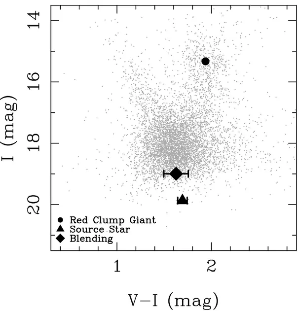
The dereddened source magnitude and color can be estimated as follows. We locate the clump in the color magnitude diagram (CMD) of stars within 20 of the source star, shown in Figure3, with the following method. The stars, which are I < 17 mag and (V − I) > 1.5 mag, were used for the clump estimate. Among them, the stars within 0.3 mag from the clump centroid were picked up. Note that the clump in the first turn was assumed. Then, the mean magnitude of I and mean color (V − I) were calculated using the stars within 0.3 mag and replaced as the new clump centroid. This was iterated until the clump centroid position is converged. Therefore, we find the clump as [I, (V − I)]clump = (15.31, 1.91). The best model source brightness and color are obtained as [I, (V − I)]S = (19.82, 1.69) from the fits. With a 0.05 mag correction due to blending by fainter stars in this crowded field (Bennett et al. 2010), this yields
[I, (V − I)]S− [I, (V − I)]clump = (4.51,−0.22). (2) We adopt the dereddened RCG magnitude MI,0,clump =−0.25 and color (V −I)0,clump= 1.04
fromBennett et al.(2008), which is based onGirardi & Salaris(2001) andSalaris & Girardi
(2002). Rattenbury et al. (2007) find that the clump in this field lies 0.12 mag in the foreground of the Galactic center, which we take to be at R0 = 8.0± 0.3 kpc (Yelda et al.
2010). Hence, the distance modulus of the clump is DM = 14.40. This yields a dereddened RCG centroid in this field of
[I, (V − I)]clump,0 = (14.15, 1.04) . (3)
Assuming that the source suffers the same extinction as the clump, we use the best fit source magnitude and color to obtain the dereddened values for the source,
[I, (V − I)]S,0 = (14.15, 1.04) + (4.51,−0.22)
= (18.66, 0.82). (4)
A comparison of (V−I)S,0estimated by this method to 14 spectra of microlensed source stars at high magnification (Bensby et al. 2010) suggests that (V − I)S,0 is determined with an uncertainty of 0.06 mag. For the uncertainty in IS,0, we estimate uncertainties of 0.08 from R0, 0.05 from the Galactic bulge RCG centroid, and 0.05 from the Rattenbury et al.(2007) offset from the Galactic center, which when added in quadrature yields a total uncertainty of 0.11 mag.
Equation (3) implies extinction of AI = 1.26±0.11 and reddening E(V −I) = 0.87±0.08,
which is consistent within the error with E(V−I) = 0.97±0.03 from the OGLE-II extinction map (Sumi 2004).
5. Measurement of the Angular Einstein Radius, θE
The sharp caustic crossing features in the MOA-2009-BLG-319 light curve resolve the finite angular size of the source star, and these finite source effects allow us to determine the angular Einstein radius θEand the lens-source relative proper motion µrel = θE/tE. Following
Yoo et al.(2004), we use the dereddened color and magnitude of the source [I, (V−I)]S,0from Eq. (4). Next, we obtain the source angular radius using the source V and K magnitude. We estimate (V − K)0 from (V − I)0 and theBessell & Brett(1988) color-color relations for dwarf stars,
[K, (V − K)]S,0 = (17.67, 1.81)± (0.14, 0.15). (5)
We also estimate the K magnitude using IRSF data, KS,0= 18.09± 0.42. This is consistent
with but less accurate than the K magnitude estimated from (V − I)0. So, we use K magnitude estimated from (V − I)0. For main sequence stars, the relationship between color, brightness, and a star angular radius θ∗ was determined by Kervella et al. (2004) to be
log(2θ∗) = 0.0755(V − K) + 0.5170 − 0.2K, (6)
which with K and (V − K) from Eq. (5) implies
θ∗ = 0.66± 0.06 µas. (7)
The fit parameter ρ ≡ θ∗/θE is source star angular radius in units of the angular Einstein
radius. Thus, the angular Einstein radius θE is θE = θ∗
ρ = 0.34± 0.03 mas. (8)
Therefore, the source-lens relative proper motion µ is
µ = θE
tE = 7.52± 0.65 mas yr
−1. (9)
6. Microlensing Parallax Effect
The event time scale is not long, tE = 16.6 days, so one does not expect to detect the
the very sharp third peak was observed simultaneously from Australia, New Zealand, and Hawaii, i.e., along two nearly perpendicular base lines of length, 0.36R⊕and 1.25R⊕, respec-tively. Therefore, there is some chance that these data will reveal a signal due to terrestrial microlensing parallax (Hardy & Walker 1995; Holz & Wald 1996;Gould et al. 2009).
Microlensing parallax is usually described by the parallax parameter, πE, which is the
amplitude of the two-dimensional microlens parallax vector, and the two components of this vector are denoted by πE,E and πE,N, which are the east and north components of the vector
on the sky. The microlens parallax vector has the same direction as the lens-source proper motion, perpendicular to the line of sight. It is related to the lens-source relative parallax
πrel and the angular Einstein radius θE (Gould 2000) by πE =
πrel θE
, πrel = πL− πS, (10)
where πL and πS are the lens and the source parallaxes, respectively.
Our initial search for microlensing parallax included both the orbital and terrestrial effect, as is necessary for a physically correct model. Our initial fits indicated a weak mi-crolensing parallax signal, so we searched for orbital parallax and terrestrial signals sep-arately, in order to determine which type of parallax signal is being seen and to test for possible systematic errors. We must also consider alternative model solutions due to the
u0 > 0 ↔ u0 < 0 degeneracy first noted by Smith et al. (2003). As the model results listed
in Table 2 indicate, orbital parallax can improve the fit χ2 by only ∆χ2 = 0.6, with two
additional parameters, which is not, at all, significant. The best terrestrial parallax model, however, does give a formally significant χ2 improvement of ∆χ2 = 6.2, but this improvement
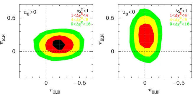
decreases to ∆χ2 = 6.1 for the best physical (terrestrial plus orbital) parallax model. With two additional parameters, this is formally significant at almost the 95% confidence level. Figure 4 shows the ∆χ2 contours for microlensing parallax fits to the MOA-2009-BLG-319
light curve.
The best fit parallax model has u0 > 0 and (πE,E, πE,N) = (−0.15, 0.15) ± (0.07, 0.05),
while the best fit u0 < 0 model has a χ2 value that is larger than the best fit u0 > 0 solution
by 1.7 and only an improvement of ∆χ2 = 4.4 over the best fit non-parallax solution. Thus,
the best u0 < 0 model is neither a significant improvement over the best non-parallax model
nor significantly worse than the best parallax model. We find that χ2 improvement for the
best fit parallax model comes from Mt. John observatory (MOA-II 1.8m and Canterbury 0.6m) telescopes alone, with a total χ2 improvement ∆χ2 = 7.3, while the contribution of all the other data sets is ∆χ2 =−1.2 (i.e. the parallax model is disfavored). One would expect
that χ2 should improve for the many other data sets, and the fact that it does not suggests
If we assume that the scalar parallax measurement of πEis correct, then it implies that
the lens system is located in the inner Galactic disk. Due to the flat rotation curve of the Galaxy, the stars at this location are rotating much faster than the typical line of sight to a Galactic bulge star. As a result, the direction of the parallax vector (which is parallel to the lens-source relative velocity) is most likely to be in the direction of Galactic rotation, which is ∼ 30◦ East of North. This is similar to the direction of the parallax vector for the best
u0 < 0 model, but it is roughly perpendicular to that for the u0 > 0 model. So, the u0 > 0
solution appears to be disfavored on a priori grounds.
Because of the low significance of the microlensing parallax signal and the indications of possible systematic problems with the measurement of the parallax parameters, we will use only an upper limit on the microlensing parallax effect in our analysis.
7. The Lens Properties
We can place lower limits on the lens mass and distance with our measured angular Einstein radius, θE, and our upper limit on the amplitude of the microlens parallax vector, πE. The lens mass is given by
M = θE κπE
, (11)
where κ = 4G/(c2 AU) = 8.1439 mas M −1. With our upper limit from the previous section,
πE < 0.5, gives a lower limit on the total mass of the lens system, M > 0.08M . This implies that the lens primary is more massive than a brown dwarf and must be a star or stellar remnant. From Eq. (10), this implies that the source-lens relative parallax is
πrel < 0.17 mas.
The vast majority of source stars for microlensing events seen towards the bulge are stars in the bulge, and the MOA-2009-BLG-319 source magnitude and colors are consistent with a bulge G-dwarf source. So, it is reasonable to assume that the source is a bulge star with a distance of DS ≈ 8.0 kpc. This implies that the lens parallax is πL = πrel+ πS < 0.30
mas, from Equation (10). The lens parallax is related to the distance by πL = 1 AU/DL, so
a lower limit on the lens distance is DL > 3.33 kpc.
An upper limit on the lens mass may be obtained if we assume that the planetary host star is a main sequence star and not a stellar remnant. We can consider the blended flux seen at the same location of the source beyond the measured source flux from the microlensing models. If we attribute this blended flux to a single star, we can follow the reasoning of
Section4 in order estimate the dereddened magnitude of the blend star
(I, V − I)b,0 = (17.78, 0.75)± (0.12, 0.14) , (12) under the (conservative) assumption that the blend star lies behind all the foreground dust. We can now use this as an upper limit on the brightness of a main sequence lens star. From
Schmidt-Kaler (1982) and Bessell & Brett (1988), we find an upper limit on the host star mass of M < 1.14M .
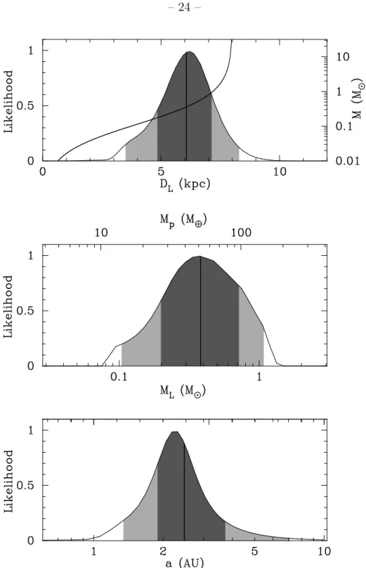
As we found finite source effects in the light curve, we can break out one degeneracy of the lens star mass M , distance DLand velocity v. We calculated the probability distribution
from Bayesian analysis by combining this equation and the measured values of θE and tE
with the Galactic model (Han & Gould 2003) assuming the distance to the Galactic center is 8 kpc. We included the upper limit of microlens parallax amplitude. A constraint of the upper limit for blending light was also included for the lens mass upper limit. The probability distribution from a Bayesian analysis is shown in Figure 5. The host star is a K or M-dwarf star with a mass of ML = 0.38+0.34−0.18 M and distance DL = 6.1+1.1−1.2 kpc,
planetary mass Mp = 50+44−24 M⊕ and projected separation r⊥ = 2.0+0.4−0.4 AU. The physical
three-dimensional separation, a = 2.4+1.2−0.6 AU, was estimated by putting a planetary orbit at random inclination, eccentricity and phase (Gould & Loeb 1992).
8. Discussion and Conclusion
We have reported the discovery of a sub-Saturn mass planet in the light curve of mi-crolensing event, MOA-2009-BLG-319. This event was observed by 20 telescopes, the largest number of telescopes to participate in a microlensing planet discovery to date. The lens system has a mass ratio q = (3.95±0.02)×10−4 and a separation d = 0.97537±0.00007 Ein-stein Radii. The lens-source relative proper motion was determined to be µrel= 7.52± 0.65
mas yr−1 from the measurement of finite source effects. A slightly better light curve fit can be obtained when the (terrestrial) microlensing parallax effect is included in the model, yield-ing an improvement of ∆χ2 = 6.1. This is very marginal statistical significance, and there
are indications that systematic errors may influence the result. So, we use our microlensing parallax analysis to set an upper limit of πE < 0.5.
The probability distribution estimated from a Bayesian analysis indicates that the lens host star mass is ML = 0.38+0.34−0.18 M with a sub-Saturn-mass planet, Mp = 50+44−24 M⊕ and
the physical three-dimensional separation a = 2.4+1.2−0.6 AU. The distance of the lens star is
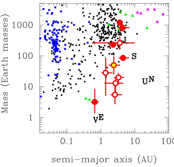
DL = 6.1+1.1−1.2 kpc. The known microlensing exoplanets are summarized in Figure 6 and
estimated to be at asnow = 2.7 AU M/M . This is similar to the separation of other planets
found by microlensing (Sumi et al. 2010).
There is some indications of low level systematic deviations from the best fit model remaining in the light curve, near the third and fourth caustic crossing features (see the bottom panel residuals in Fig.1), which does not affect the results in this analysis. These systematic light curve deviations might be caused by orbital motion of the lens, a second planet, or systematic photometry errors. A more detailed analysis will be performed in the future when the adaptive optics images from the Keck telescope were reduced, and this analysis may shed more light on the mass and distance of the host star.
The next few years are expected to see an increase in the rate of microlensing planet discoveries. The OGLE group has started the OGLE-IV survey with their new 1.4 deg2 CCD camera in March, 2010. This will allow OGLE to survey the bulge at a cadence almost as high as that of MOA-II, but with better seeing that should yield a substantial increase in the rate of microlensing planet discoveries. MOA also plans an upgrade to a ∼ 10 deg2 MOA-III CCD camera in a few years, which will allow an even higher cadence Galactic bulge survey. The Korean Microlensing Telescope Network (KMTNet) is funded to dramatically increase the longitude coverage of microlensing survey telescopes. They plan three wide FOV telescopes to go in South Africa, Australia and South America. When these telescopes come online, we anticipate another dramatic increase in the microlensing planet discovery rate.
The MOA project and a part of authors were supported by the Grant-in-Aid for Scientic Research, the grant JSPS20340052, JSPS18253002, JSPS Research fellowships, the Global COE Program of Nagoya University ”Quest for Fundamental Principles in the Universe” from JSPS and MEXT of Japan, the Marsden Fund of New Zealand, the New Zealand Foundation for Research and Technology, and grants-in-aid from Massey University and the University of Auckland. N.M. was supported by JSPS Research Fellowships for Young Sci-entists. T.S. was supported by the grant JSPS20740104. D.P.B. was supported by grants NNX07AL71G and NNX10AI81G from NASA and AST-0708890 from the NSF. A.G. and S.D. were supported in part by NSF AST-0757888. A.G., S.D., S.G., and R.P. were sup-ported in part by NASA NNG04GL51G. Work by S.D. was performed in part under contract with the California Institute of Technology (Caltech) funded by NASA through the Sagan Fellowship Program. J.C.Y. was supported by a NSF Graduate Research Fellowship. This work was supported by the Creative Research Initiative program (2009-0081561) of the Na-tional Research Foundation of Korea. Astronomical research at Armagh Observatory was supported by the Department of Culture, Arts and Leisure (DCAL), Northern Ireland, UK. F.F., D.R. and J.S. acknowledge support from the Communaut´e fran¸caise de Belgique – Actions de recherche concert´ees – Acad´emie universitaire Wallonie-Europe
REFERENCES Albrow, M. D., et al. 2009, MNRAS, 397, 2099
Alcock, C., et al. 1995, ApJ, 454, L125 Beaulieu, J.-P., et al. 2006, Nature, 439, 437 Bennett, D. P. 2010, ApJ, 716, 1408
Bennett, D. P., & Rhie, S. H. 1996, ApJ, 472, 660 Bennett, D. P., et al. 2008, ApJ, 684, 663
Bennett, D. P., et al. 2010, ApJ, 713, 837 Bensby, T., et al. 2010, A&A, 512, A41
Bessell, M. S., & Brett, J. M. 1988, PASP, 100, 1134 Bond, I. A., et al. 2001, MNRAS, 327, 868
Bond, I. A., et al. 2004, ApJ, 606, L155 Bramich, D. M. 2008, MNRAS, 386, L77 Claret, A. 2000, A&A, 363, 1081
Cumming, A., et al. 2008, PASP, 120, 531 Dong, S., et al. 2009, ApJ, 698, 1826
Doran, M., & Mueller, C. M. 2004, J. Cosmology Astropart. Phys., 9, 3 Gaudi, B. S., et al. 2008, Science, 319, 927
Girardi, L., & Salaris, M. 2001, MNRAS, 323, 109 Gould, A. 1992, ApJ, 392, 442
Gould, A. 2000, ApJ, 542, 785 Gould, A. 2004, ApJ, 606, 319
Gould, A., & Loeb, A. 1992, ApJ, 396, 104 Gould, A., et al, 2006, ApJ, 644, L37
Gould, A., et al. 2009, ApJ, 698, L147 Gould, A., et al. 2010, ApJ, 720, 1073
Griest, K., & Safizadeh, N. 1998, ApJ, 500, 37 Han, C., & Gould, A. 2003, ApJ, 592, 172
Hardy, S. J., & Walker, M. A. MNRAS, 276, L79 Holz, D. E., & Wald, R. M. 1996, ApJ, 471, 64 Ida, S., & Lin, D. N. C. 2004, ApJ, 616, 567 Janczak, J., et al. 2010, ApJ, 711, 731
Kennedy, G. M., & Kenyon, S. J. 2008, ApJ, 673, 502 Kervella, P., et al. 2004, A&A, 426, 297
Lecar, M., Podolak, M., Sasselov, D., & Chiang, E. 2006, ApJ, 640, 1115 Rattenbury, N. J., et al., 2002, MNRAS, 335, 159
Rattenbury, N. J., Mao, S., Sumi, T., & Smith, M. C. 2007, MNRAS, 378, 1064 Refsdal, S. 1966, MNRAS, 134, 315
Rhie, S. H., et al. 2000, ApJ, 533, 378 Sako, T., et al. 2008, Exp. Astron., 22, 51
Salaris, M., & Girardi, L. 2002, MNRAS, 337, 332
Schmidt-Kaler, Th. 1982, in Landolt-B¨ornstein: Numerical Data and Functional Relation-ships in Science and Technology, Vol 2b, ed. K. Schaifers & H. H. Voigt (Berlin: Springer)
Smith, M. C., Mao, S., & Paczy´nski, B. 2003, MNRAS, 339, 925 Sumi, T. 2004, MNRAS, 349, 193
Sumi, T., et al. 2003, ApJ, 591, 204 Sumi, T., et al. 2010, ApJ, 710, 1641 Udalski, A. 2003, Acta Astron., 53, 291
Udalski, A., et al. 2005, ApJ, 628, L109 Verde, L., et al. 2003, ApJS, 148, 195 Wambsganss, J. 1997, MNRAS, 284, 172 Wozniak, P. R. 2000, Acta Astron., 50, 421 Yelda, S., et al. 2010, arXiv1002.1729 Yoo, J., et al. 2004, ApJ, 603, 139
Fig. 1.— The light curve of planetary microlensing event MOA-2009-BLG-319. The top panel shows the data points and the best fit model light curve with finite source and limb darkening effects. The three lower panels show close-up views of the four caustic crossing light curve regions and the residuals from the best fit light curve. The photometric measurements from MOA, B&C, Auckland, Bronberg, CAO, CTIO, Farm Cove and LOAO are plotted as filled dots with colors indicated by the legend in the top panel. The other data sets are plotted with open circles. The data sets of µFUN Bronberg and SSO have been averaged into 0.01 day bins, and the RoboNet FTN and FTS data sets are shown in 0.005 day bins, for clarity.
Fig. 2.— The caustic is plotted in solid curve for the MOA-2009-BLG-319 best fit model, and the dash line indicates the source star trajectory. The circle represents the source star size. The source star crosses the caustic curve four times, with peak magnification of Amax= 205
Fig. 3.— (V − I, I) color magnitude diagram of the stars within 20 of the MOA-2009-BLG-319 source using µFUN CTIO data calibrated to OGLE-II. The filled triangle and square indicate the source and blend stars, respectively, assuming that the blended light comes from a single star. The filled circle indicates the center of the red clump giant distribution.
Fig. 4.— The contours of ∆χ2=1, 4, 9, 16 with orbital and terrestrial parallax parameters.
The left panel is the result with u0 > 0 and the right panel is with u0 < 0. The best fit
result with u0 > 0 is better than u0 < 0 about ∆χ2 = 1.7. Furthermore, the best fit model
Fig. 5.— Probability distribution from a Bayesian analysis for the distance, DL, mass, ML,
and the physical three dimensional separation a. The vertical solid lines indicate the median values. The dark and light shaded regions indicate the 68% and 95% limits. The solid curve in the top panel indicates the mass-distance relation of the lens from the measurement of θE
Fig. 6.— Exoplanets as a function of mass vs. semi-major axis. The red circles with error bars indicate planets found by microlensing. The filled circles indicate planets with mass measurements, while open circles indicate Bayesian mass estimates. MOA-2009-BLG-319Lb is indicated by the gold-filled open circle. The black dots and blue squares indicate the planets discovered by radial velocities and transits, respectively. The magenta and green triangles indicate the planets detected via direct imaging and timing, respectively. The non-microlensing exoplanet data were taken from The Extrasolar Planets Encyclopaedia (http://exoplanet.eu/). The planets in our solar system are indicated with initial letters.
Table 1. Limb darkening coefficients for the source star with effective temperature
Teff=5500 K, surface gravity log g=4.5 and metallicity log[M/H]=0.0 (Claret 2000).
filter color V R I J H K
c 0.3866 0.2556 0.1517 -0.0234 -0.2154 -0.1606
T able 2. The b est fit mo del parameters with v arious effects, finite source, orbital and terrestrial parallax, and u0 . The lines with ” σ ” list the 1 σ error of parameters giv en b y MCMC. HJD’ ≡ HJD-2450000. Note that the u0 con v en tions are the same as Fig. 2 of Gould ( 2004 ). χ 2 v alue is the result of the fitting with 18 data sets, whic h ha v e 7210 data p oin ts. The mo del searc h with finite source and orbital parallax effects w ere done b y a grid searc h. orbital terrestrial u0 > 0 u0 < 0 t0 tE u0 q d α ρ πE ,E πE ,N χ 2 parallax parallax HJD’ [da ys] 10 − 3 10 − 4 [rad] 10 − 3 ◦ 5006.99482 16.57 6.22 3.95 0.97537 5.7677 1.929 ·· · ·· · 7023.8 σ 0.00006 0.08 0.03 0.02 0.00007 0.0005 0.010 ·· · ·· · ◦ 5006.99485 16.56 -6.23 3.95 0.97540 0.5156 1.931 ·· · ·· · 7023.8 σ 0.00005 0.08 0.03 0.02 0.00006 0.0005 0.009 ·· · ·· · ◦ ◦ 5006.99480 16.59 6.22 3.95 0.97540 5.7673 1.929 0.40 0.30 7023.2 σ 0.00007 0.09 0.03 0.02 0.00007 0.0005 0.011 ·· · ·· · ◦ ◦ 5006.99482 16.56 -6.23 3.95 0.97534 0.5155 1.931 0.40 -0.30 7023.4 σ 0.00006 0.08 0.03 0.02 0.00007 0.0005 0.010 ·· · ·· · ◦ ◦ 5006.99477 16.61 6.21 3.94 0.97540 5.7671 1.926 -0.23 0.12 7017.6 σ 0.00006 0.08 0.03 0.02 0.00007 0.0005 0.010 0.07 0.04 ◦ ◦ 5006.99483 16.57 -6.23 3.95 0.97542 0.5161 1.931 -0.02 0.26 7019.2 σ 0.00006 0.07 0.03 0.02 0.00007 0.0005 0.010 0.04 0.07 ◦ ◦ ◦ 5006.99478 16.60 6.21 3.94 0.97540 5.7673 1.926 -0.15 0.15 7017.7 σ 0.00006 0.08 0.03 0.02 0.00007 0.0004 0.010 0.07 0.05 ◦ ◦ ◦ 5006.99481 16.56 -6.23 3.95 0.97538 0.5162 1.932 -0.04 0.23 7019.4 σ 0.00006 0.07 0.03 0.02 0.00007 0.0005 0.009 0.04 0.07
T able 3. P arameters of exoplanets disco v ered b y microlensing. MO A-2007-BLG-400Lb has tw o solutions due to a strong close/wide mo del degeneracy , and details of the MO A-2008-BLG-310Lb parameters are discussed b y Janczak et al. ( 2010 ) and Sumi et al. ( 2010 ). name Host Star Mass Distance Planet Mass Separation Mass estimated b y M L (M ) DL (kp c) M p a (A U) OGLE-2003-BLG-235Lb 0 .63 +0 .07 − 0 .09 5 .8 +0 .6 − 0 .7 2 .6 +0 .8 − 0 .6 M J 4 .3 +2 .5 − 0 .8 θE , lens brigh tness OGLE-2005-BLG-071Lb 0 .46 ± 0 .04 3 .2 ± 0 .4 3 .8 ± 0 .4 M J 3 .6 ± 0 .2 θE , πE , detection of the lens OGLE-2005-BLG-169Lb 0 .49 +0 .23 − 0 .29 2 .7 +1 .6 − 1 .3 13 +6 −8 M⊕ 2 .7 +1 .7 − 1 .4 θE , Ba y esian OGLE-2005-BLG-390Lb 0 .22 +0 .21 − 0 .11 6 .6 +1 .0 − 1 .0 5 .5 +5 .5 − 2 .7 M⊕ 2 .6 +1 .5 − 0 .6 θE , Ba y esian OGLE-2006-BLG-109Lb 0 .51 +0 .05 − 0 .04 1 .49 ± 0 .19 231 ± 19 M⊕ 2 .3 ± 0 .5 θE , πE c 86 ± 7 M⊕ 4 .5 +2 .1 − 1 .0 θE , πE OGLE-2007-BLG-368Lb 0 .64 +0 .21 − 0 .26 5 .9 +0 .9 − 1 .4 20 +7 −8 M⊕ 3 .3 +1 .4 − 0 .8 θE , Ba y esian MO A-2007-BLG-192Lb 0 .084 +0 .015 − 0 .012 0 .70 +0 .21 − 0 .12 3 .2 +5 .2 − 1 .8 M⊕ 0 .66 +0 .19 − 0 .14 θE , πE MO A-2007-BLG-400Lb 0 .30 +0 .19 − 0 .12 5 .8 +0 .6 − 0 .8 0 .83 +0 .49 − 0 .31 M J 0 .72 +0 .38 − 0 .16 / 6 .5 +3 .2 − 1 .2 θE , Ba y esian MO A-2008-BLG-310Lb 0 .67 ± 0 .14 > 6 .0 28 +58 −23 M⊕ 1 .4 +0 .7 − 0 .3 θE , Ba y esian MO A-2009-BLG-319Lb 0 .38 +0 .34 − 0 .18 6 .1 +1 .1 − 1 .2 50 +44 −24 M⊕ 2 .4 +1 .2 − 0 .6 θE , Ba y esian


![Table 1. Limb darkening coefficients for the source star with effective temperature T eff =5500 K, surface gravity log g=4.5 and metallicity log[M/H]=0.0 (Claret 2000).](https://thumb-eu.123doks.com/thumbv2/123doknet/6018700.150309/26.918.192.720.583.689/darkening-coefficients-effective-temperature-surface-gravity-metallicity-claret.webp)
