modelling groundwater flow and transport in a
cross-bedded aquifer
M. Huysmans1 and A. Dassargues1,2 (1)
Katholieke Universiteit Leuven, Department of Earth and Environmental Sciences, Applied Geology and Mineralogy
(2)
Université de Liège, Hydrogeology and Environmental Geology, Department of Architecture, Geology, Environment, and Civil Engineering (ArGEnCo)
0032 16 32 64 49 0032 16 32 29 80
1 Introduction
Sedimentological and erosional processes often result in a complex three-dimensional subsurface architecture of sedimentary structures and facies types. Such complex sedimentological heterogeneity may induce a highly heterogeneous spatial distribution of hydrogeological parameter values in porous media at differ-ent scales (Klingbeil et al., 1999) and may consequdiffer-ently greatly influence subsur-face fluid flow and solute migration (Koltermann and Gorelick, 1996). Because of the limited access to the relevant hydraulic properties, deterministic models often fall short in characterizing the subsurface heterogeneity and its inherent uncer-tainty. In recent decades, numerous stochastic approaches have been developed to overcome this problem. Most of these methods employ a variogram to character-ize the heterogeneity of the hydraulic parameters. Variograms are calculated based on two-point correlations only and therefore have some important limitations. Variograms are not able to describe realistic heterogeneity in complex geological environments. Complex geological patterns including sedimentary structures, multi-facies deposits, structures with large connectivity, curvi-linear structures, etc. cannot be characterized using only two-point statistics (Koltermann and Gorelick, 1996; Fogg et al., 1998). Moreover, variograms, as a limited and parsi-monious mathematical tool, cannot take full advantage of the possibly rich amount of geological information from outcrops (Caers and Zhang, 2004). Multiple-point geostatistics (Strebelle 2000; Strebelle 2002; Strebelle et al. 2002; Caers and Zhang 2003; Feyen and Caers , 2006) aims to overcome the limitations of the variogram. The premise of multiple-point geostatistics is to move beyond
two-point correlations between variables and to obtain (cross) correlation moments at multiple locations at a time (Strebelle and Journel, 2001). Because of the limited direct information from the subsurface, such statistical information cannot directly be obtained from samples. Instead, "training images" are used to characterize the patterns of geological heterogeneity. A training image is a conceptual explicit rep-resentation of the expected spatial distribution of hydraulic properties or facies types. The main idea is to borrow geological patterns from these training images and anchor them to the subsurface data domain. This study demonstrates how multiple-point geostatistics can be applied to determine the impact of complex geological heterogeneity on groundwater flow and transport in a real aquifer. More precisely, multiple-point geostatistics is used in this study to investigate the effect of complex small-scale sedimentary heterogeneity on the short term migra-tion of a contaminant plume and its uncertainty. This paper also shows how a training image can be constructed based on geological and hydrogeological field data.
2 Materials and method
2.1 Geological setting
The aquifer of interest is the Brussels Sands formation in Belgium. Approxi-mately 29,000,000 m³ of groundwater per year is pumped from this aquifer. The Brussels Sands display a complex geological heterogeneity and anisotropy that complicates pumping test interpretation, groundwater modeling and prediction of pollutant transport. The Brussels Sands formation is an early Middle-Eocene shal-low marine sand deposit in Central Belgium (Fig. 1). The depositional environ-ment of the Brussels Sands is studied in detail by Houthuys (1990) based on field studies and descriptions of approximately 90 outcrops and hundreds of boreholes. The Brussels Sands are a tidal sandbar deposit, deposited at the beginning of an important transgression at the southern border of the Eocene North Sea. The Brus-sels Sands display several features and sedimentary structures typical for tidal de-posits, such as important grain size variations, cross-bedding, bottomsets, foresets, mud drapes and unidirectional reactivation surfaces. Bottomset beds are approxi-mately horizontal beds consisting of finer grained sediment and form the base of most bedded beds. Mud drapes are thin layers of mud within the cross-bedded beds.
Figure 1 Map of Belgium showing Brussels Sands outcrop and subcrop area (shaded part) and
the location of the Bierbeek quarry (modified after Houthuys, 1990)
2.2 Field measurements
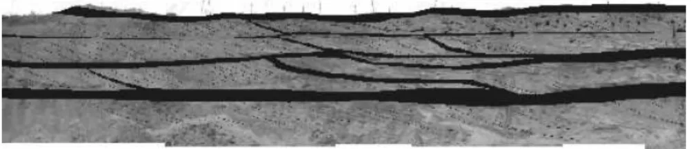
An extensive field campaign is carried out consisting of field observations of the sedimentary structures and 2750 small-scale in situ measurements of air per-meability in the Brussels Sands. The results and conclusions of this field campaign are summarized in this section. More details about this field campaign can be found in Huysmans et al., 2008. A representative Brussels Sands outcrop (Bier-beek quarry near Leuven, Belgium) is mapped in detail with regard to the spatial distribution of sedimentary structures and lithologies. Geological sketches and digital photographs from all faces of the quarry are made. A visual distinction be-tween sand-rich and clay-rich zones, hereafter called the sand facies and the silt facies respectively, is made in situ based on sediment characteristics. Figure 2 shows an interpreted photomosaic of one of the outcrops of the vertical quarry walls, corrected for perspective distortion. Thickness and dip measurements of several sedimentary features are made at various locations in the quarry and ana-lyzed statistically. Histograms of bottomset thicknesses, set thicknesses and lami-nation dipping angles measured during this measurement campaign and from Houthuys (1990) are calculated. Additionally, a total of 2750 air permeability measurements at cm-scale are carried out in situ. Permeability histograms and variograms of the sand and silt facies are calculated. Analysis of the spatial
distri-bution of sedimentary structures and permeability shows that silt facies consisting of clay-rich sedimentary features such as bottomsets and distinct mud drapes ex-hibit a different statistical and geostatistical permeability distribution compared to the sand facies. Variogram map analysis of the air permeability data shows that permeability anisotropy in the cross-bedded lithofacies is dominated by the foreset lamination orientation. The results show that small-scale sedimentary heterogene-ity has a dominant control on the spatial distribution of the hydraulic properties and induces permeability heterogeneity and anisotropy.
Figure 2 Interpreted photomosaic of quarry wall showing the silt facies consisting of clay-rich
bottomsets and distinct mud drapes in black. Height of quarry wall is approximately 4 to 5 m (Huysmans et al., submitted).
2.3 Training image construction
To demonstrate the need for “training images” in multiple-point geostatistics, this section first briefly recalls the mathematical basis behind multiple-point geo-statistics. The remainder of this section describes the training image construction process for this study. Consider an attribute S, taking J possible states {sj, j=1…
J}. S can be a categorical property, e.g. facies, or a continuous value such as
per-meability, with its interval of variability discretized into J classes. A data event dn
of size n centered at location u is constituted by (1) the data geometry defined by the n vectors {hα, α=1… n} and (2) the n data values {s(u+hα), α=1… n}. A data template τn comprises only the previous data geometry. The categorical transform
of the variable S at location u is defined as:
( )
;
0
if
( )
( )
1
if
j jS
s
I
j
S
s
=
=
≠
u
u
u
The multiple-point statistics are probabilities of occurrence of the data events
dn={S(uα)=sj,α, α=1… n}, i.e. probabilities that the n values s(u1) … s(uj) are
jointly in the respective states sj,1 … sj,n. For any data event dn, that probability is
{ }
{
( )
,}
(
)
1Prob
Prob
;
1...
E
,
n n jd
S
αs
αn
I
αj
α αα
=
=
=
=
=
Π
u
u
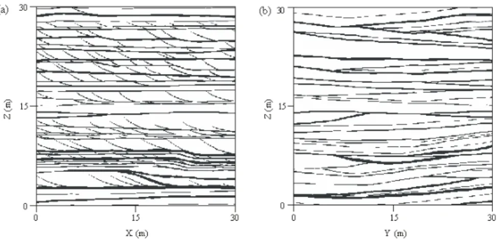
Such multiple-point statistics or probabilities cannot be inferred from sparse field data. Their inference requires a training image depicting the expected pat-terns of geological heterogeneities. Training images can be obtained from obser-vations of outcrops, geological reconstructions and geophysical data (Strebelle and Journel, 2001). In this study, training images are constructed based on observa-tions of outcrops. 2D vertical training images of clay and sand occurrence in dif-ferent orientations are constructed based on field photographs and observations of the geometry and dimensions of the sedimentary structures. The 2D training im-ages are composite sketches composed of smaller scale photographs and field sketches conditioned by the histograms of set thicknesses, bottomset thicknesses and lamination angles. The training image size is 30 m by 30 m. To capture the thin clay drapes, a small grid cell size of 0.05 m by 0.05 m is adopted so that the training image consists of 360000 grid nodes. Figure 3 shows the 2D training im-ages in the N40°E direction and the approximately perpendicular N45°W tion. These training images show that the facies distribution in the N40°E direc-tion is rather complex while almost horizontal layering is observed in the perpendicular direction. Since the facies changes in the N45°W direction are so limited compared to the other direction, 2D analyses are carried out in the remain-der of this paper only consiremain-dering the training image shown in Figure 3a.
Figure 3 Vertical 2D training image of 30 m x 30 m in (a) N40°E direction and (b) N45°W
2.4 Multiple-point geostatistical facies realizations
Multiple-point statistics are borrowed from the training image to simulate mul-tiple realizations of silt and sand facies occurrence using the single normal equa-tion simulaequa-tion (SNESIM) algorithm (Strebelle, 2002). Snesim is a pixel-based sequential simulation algorithm that obtains multiple-point statistics from the training image, exports it to the geostatistical numerical model and anchors it to the actual subsurface hard and soft data. For each location along a random path the data event dn consisting of the set of local data values and their spatial
configura-tion is recorded. The training image is scanned for replicates that match this event to determine the local conditional probability that the unknown attribute S(u) takes any of the J possible states given the data event dn, as
( )
{
}
{
( )
{
( )
( )
,}
}
,Prob
and
;
1...
Prob
Prob
;
1...
j j j n jS
s
S
s
n
S
s d
S
s
n
α α ε αα
α
=
=
=
=
=
=
=
u
u
u
u
The denominator can be inferred by counting the number of replicates of the conditioning data event found in the training image. The numerator can be ob-tained by counting the number of those replicates associated to a central value
S(u) equal to sk. A maximum data search template is defined to limit the geometric
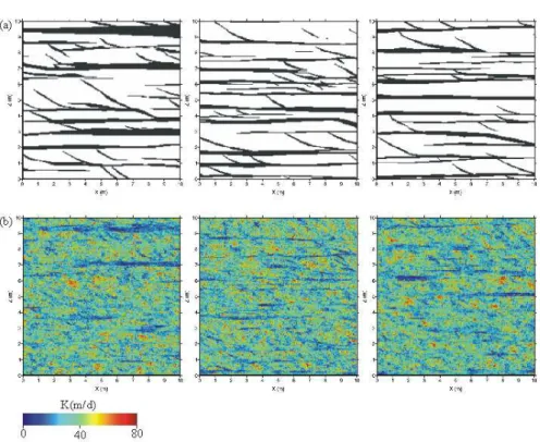
extent of those data events. SNESIM requires reasonable CPU demands by scan-ning the traiscan-ning image prior to simulation and storing the conditional probabili-ties in a dynamic data structure, called the search tree. The theory and algorithm behind SNESIM are described in Strebelle, 2002. Descriptions of SNESIM pa-rameters are in Liu, 2006; Strebelle and Remy, 2005 and Strebelle 2003. The computation time and pattern reproduction quality of SNESIM realizations are strongly dependent on the input parameters selection (Liu, 2006). In this particular case, the input parameters selection is complicated by the nature of the heteroge-neity. The combination of thin clay drapes and relatively large structures results in a large training image size with a small grid cell size. This requires a large tem-plate size and thus a large CPU and RAM demand. To optimally choose the input parameter values, a sensitivity analysis of the input parameters to pattern repro-duction and computation time is carried out. The simulation grid is 10 m by 10 m and consists of 40000 grid cells of 0.05 m by 0.05 m. Template shape, template dimension and multi-grid number prove to be the most influential parameters. An optimal compromise between pattern reproduction and computation time for this case is found for simulations using an elliptical template of 21 by 3 nodes, 6 multi-grids, 48 previously simulated nodes in the sub-grid approach, a re-simulation threshold of 50 and 6 re-simulations iterations. A total of 150 SNESIM realiza-tions of 10 m by 10 m are simulated using the optimal input parameter selection. Figure 4 a shows three example SNESIM facies realizations.
Figure 4 (a) Three example 2D vertical SNESIM facies realizations (white = sand facies, black =
silt facies); (b) Corresponding hydraulic conductivity (m/d) realizations
2.5 Intrafacies permeability simulation
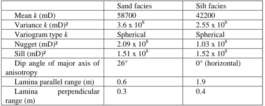
Intrafacies permeability variability within the sand and silt facies is simulated using conventional variogram-based geostatistical methods based on histograms and variograms obtained from the in situ air permeability measurements. The simulation algorithm used in this study is direct sequential simulation with histo-gram reproduction (Oz et al., 2003). The input statistics and variohisto-gram parameters of permeability for both facies are presented in Table 1. Air permeability realiza-tions are converted into hydraulic conductivity realizarealiza-tions to serve as input to a local groundwater flow model. In this way, intrafacies hydraulic conductivity of the 150 facies realizations is simulated. Figure 4b shows the hydraulic conductiv-ity realizations of the facies realizations of figure 4a. The silt facies are visible in the hydraulic conductivity realizations as areas with lower hydraulic conductivity. The low conductivity zones are however no continuous flow barriers since the sand and silt permeability distributions are overlapping.
Table 1 Statistical and variogram parameters of permeability in mD (milliDarcy) for the sand
and silt facies (values from Huysmans et al., 2008)
Sand facies Silt facies
Mean k (mD) 58700 42200
Variance k (mD)² 3.6 x 10⁸ 2.55 x 10⁸ Variogram type k Spherical Spherical Nugget (mD)² 2.09 x 10⁸ 1.03 x 10⁸
Sill (mD)² 1.51 x 10⁸ 1.52 x 10⁸
Dip angle of major axis of anisotropy
26° 0° (horizontal) Lamina parallel range (m) 0.6 1.9
Lamina perpendicular range (m)
0.3 0.4
2.6 Groundwater flow and transport model
The simulated hydraulic conductivity realizations are used as input to a groundwater flow and transport model to investigate the effect of the small-scale sedimentary heterogeneity on early contaminant plume migration. The contami-nant source is a hypothetical source. The location of this hypothetical source in the real world, and hence the location of the model, is not specified and could be anywhere in the Brussels Sands where the type of structures displayed in the train-ing image occur. The model is a small-scale and short-term (3-day) 2D vertical model of 10 m by 10 m, discretized into very small grid cells of 5 cm by 5 cm in order to represent the thin clay drapes present in the Brussels Sands. Constant head boundary conditions are applied to all boundaries so that the average hori-zontal gradient is 10 m/km and the average vertical hydraulic gradient is 5 m/km corresponding to observed gradients in the Brussels Sands. Porosity of the sand and silt facies are both assumed to be 30% since no facies specific porosity infor-mation is available. A hypothetical source of an inert contaminant is assumed at the surface at x=2 with an arbitrarily chosen flow rate of 1000 l/day and an arbi-trarily chosen source concentration of 1000 mg/l. Corresponding to the very small grid cell dimension, a very low longitudinal dispersivity value of 0.01 m is chosen based on extrapolation of the relationships between dispersivity and the scale of observation from Gelhar et al. (1992). Transverse dispersivity is taken one order of magnitude smaller than longitudinal dispersivity (Zhen and Bennett, 1995). Dispersivity values are assumed equal in both facies since no facies specific dis-persivity information is available. The differential equations describing groundwa-ter flow are solved by MODFLOW (McDonald and Harbaugh 1988), a block-centered finite-difference method based software package. Transport by advection
and dispersion is simulated with MT3DMS (Zheng and Wang 1999), using the high-order finite-volume TVD solver. The Courant number used for determination of the time step size for transport calculations is 0.75. This groundwater flow and transport model is run 150 times for the 150 simulated hydraulic conductivity re-alizations. The distributions and uncertainty of the following three relevant output parameters are calculated and studied: (1) the maximum solute concentration after 3 days, (2) the maximum depth where a concentration of 1 mg/l is reached after 3 days and (3) the maximum horizontal distance to the source where a concentration of 1 mg/l is reached after 3 days. The convergence of the output parameter statis-tics in terms of the number of simulations is also studied in order to check whether 150 simulations are sufficient.
3 Results and discussion
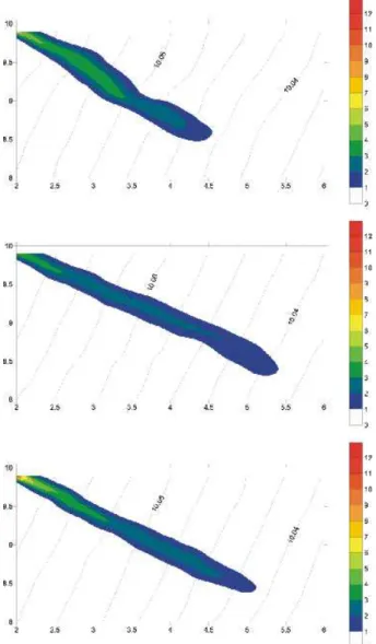
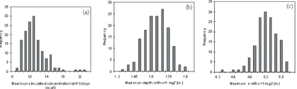
Figure 5 zooms in on the calculated contaminant plume for the three hydraulic conductivity realizations of Figure 4 and shows simulated hydraulic head contours and contaminant concentrations for t = 3 days. These figures show a different plume shape and extent and different maximum concentrations for the different hydraulic conductivity realizations. Figure 6 shows histograms of the three rele-vant output parameters defined in the previous section. The maximum simulated solute concentration for t = 3 days varies between 6.3 and 22.0 mg/l and shows a slightly skewed distribution with a mean of 10.7 mg/l and a standard deviation of 2.7 mg/l. The maximum depth with a concentration of 1 mg/l for t = 3 days varies between 1.3 and 1.9 m and shows a symmetric distribution with a mean of 1.6 m and a standard deviation of 0.1 m. The maximum horizontal distance to the source with a concentration of 1 mg/l for t = 3 days varies between 4.3 and 5.6 m and shows a slightly skewed distribution with a mean of 5.2 m and a standard devia-tion of 0.2 m. The contaminant plumes of different realizadevia-tions thus have signifi-cantly different characteristics. The largest maximum simulated solute concentra-tion is more than three times larger than the smallest maximum simulated solute concentration. The largest maximum depth with c = 1 mg/l is almost 50% larger than the smallest maximum depth with c = 1 mg/l and the largest maximum hori-zontal distance with c = 1 mg/l is 30% larger than the smallest maximum horizon-tal distance with c = 1 mg/l. These results show that the uncertainty on the spatial facies distribution and intrafacies hydraulic conductivity distribution results in a significant uncertainty on the calculated concentration distribution. Especially the maximum simulated concentration value can vary strongly among the different in-put hydraulic conductivity realizations.
Figure 5 Simulated hydraulic head contours and contaminant concentrations for t = 3 days for
the three realizations of figure 4
4 Conclusions
This study applies multiple-point geostatistics in the field of hydrogeology on a real aquifer. This study demonstrates how a training image can be constructed
based on geological and hydrogeological field data and how multiple-point geosta-tistics can be applied to determine the impact of complex geological heterogeneity on groundwater flow and transport in a real aquifer. Application of the proposed approach of a hypothetical contaminant case in Brussels Sands shows that the un-certainty on the spatial facies distribution and intrafacies hydraulic conductivity distribution results in a significant uncertainty on the calculated concentration dis-tribution. The small-scale sedimentary heterogeneity in the Brussels Sands has a significant effect on the calculated concentration distribution and using a homoge-neous model instead of a heterogehomoge-neous model could lead to significant error in the prediction of contaminant plume migration and concentrations. This shows that the type of heterogeneity encountered in the Brussels Sands may have a sig-nificant effect on contaminant transport and should be taken into account in groundwater contamination studies.
Figure 6 Histograms of (a) maximum solute concentration after 3 days, (b) maximum depth where a concentration of 1 mg/l is reached after 3 days and (c) maximum horizontal distance to the source where a concentration of 1 mg/l is reached after 3 days.
Acknowledgements
The authors wish to acknowledge the Fund for Scientific Research – Flanders for providing a Postdoctoral Fellowship to the first author.
References
Bronders, J., 1989. Bijdrage tot de geohydrologie van Midden België door middel van geo-statistische analyse en een numeriek model. PhD thesis, Vrije Universiteit Brussel, Brussel.
Caers J. and Zhang T., 2004, Multiple-point geostatistics: a quantitative vehicle for inte-grating geologic analogs into multiple reservoir models. In: Integration of outcrop and modern analog data in reservoir models, AAPG memoir 80, p. 383-394.
Feyen, L. and J. Caers, 2006, Quantifying geological uncertainty for f low and transport modeling in multi-modal heterogeneous formations, Advances in Water Resources, 29(6), 912-929
Fogg G.E., Noyes C.D. and Carle S.F., 1998, Geologically based model of heterogeneous hydraulic conductivity in an alluvial setting, Hydrogeology Journal 6(1), 131-143. Houthuys R., 1990, Vergelijkende studie van de afzettingsstruktuur van getijdenzanden uit
het Eoceen en van de huidige Vlaamse banken. Aard. Mededelingen 5, Leuven Univ. Press, p. 137.
Huysmans M., Peeters L., Moermans G. and Dassargues A., 2008, Relating small-scale sedimentary structures and permeability in a cross-bedded aquifer, Journal of Hydrology 361(1-2), 41-51.
Koltermann, C.E., Gorelick, S., 1996. Heterogeneity in sedimentary deposits: a review of structure imitating, process-imitation, and descriptive approaches. Water Resour. Res. 32 (9), 2617–2658.
Klingbeil, R., Kleineidam, S., Asprion, U., Aigner, T., Teutsch, G., 1999. Relating Lithofa-cies to HydrofaLithofa-cies: Outcrop-Based Hydrogeological Characterisation of Quaternary Gravel Deposits. Sediment. Geol. 129 (3-4), 299-310.
Liu Y., 2006, Using the Snesim program for multiple-point statistical simulation, Com-puters & GeosciencesVolume 32(10), 1544-1563.
McDonald, M. G. and Harbaugh, A. W. (1988). A modular three-dimensional finite-difference ground-water flow model. Technical report, U.S. Geol. Survey, Reston, VA. Oz B., Deutsch C.V., Tran T.T. and Xie Y., 2003, DSSIM-HR: A FORTRAN 90 program
for direct sequential simulation with histogram reproduction, Computers & Geo-sciences,Volume 29(1), 39-51.
Strebelle, S., 2000, Sequential simulation drawing structures from training images, Doc-toral dissertation, Stanford University, USA, 164 p.
Strebelle, S. and Journel, A, 2001, Reservoir Modeling Using Multiple-Point Statistics: SPE 71324 presented at the 2001 SPE Annual Technical Conference and Exhibition, New Orleans, September 30-October 3.
Strebelle, S., 2002, Conditional simulation of complex geological structures using multiple-point statistics: Math. Geol., v. 34, p. 1–22.
Strebelle, S., 2003, New multiple-point statistics simulation implementation to reduce memory and CPU-demand, in Proceedings to the IAMG 2003, Portsmouth, UK, Sep-tember 7–12.
Strebelle, S., and Remy, N., 2005. Post-processing of multiple-point geostatistical models to improve reproduction of training patterns, in Leuangthong, O., and Deutsch, C. V., eds., Geostatistics Banff 2004, vol. 2: Springer, Dordrecht, p. 979–987 .
Zheng, C., and G.D. Bennett, 1995, Applied Contaminant Transport Modeling, Theory and Practice, John Wiley & Sons, New York, 433 pp.
Zheng C, Wang PP. MT3DMS, a modular three-dimensional multi-species transport model for simulation of advection, dispersion and chemical reactions of contaminants in groundwater systems. Documentation and user’s guide. US Army Engineer Research and Development Center Contract Report SERDP-99-1, Vicksburg, MS, 1999