Trends in regional jobs-housing proximity based on the minimum
1
commute: the case of Belgium
2
Ismaïl Saadia, Kobe Boussauwb, Jacques Tellera, Mario Coolsa,∗
3
aUniversity of Liège, ArGEnCo, Local Environment Management & Analysis (LEMA) Quartier Polytech 1, Allée de la
4
Découverte 9, BE-4000 Liège, Belgium
5
bVrije Universiteit Brussel, Department of Geography, Cosmopolis Centre for Urban Research, Pleinlaan 2, BE-1050 Brussels,
6
Belgium
7
Abstract
8
This paper investigates recent trends in the efficiency of the Belgian territorial structure in terms of
9
commuting, at both the urban and regional scales. The minimum commute distance (MCD) and excess
10
rate (ER) are used to compare observed home-to-work trip lengths with an "optimal" alternative commuter
11
pattern in which the sum of the distance traveled by the working population is minimized. The MCD is a
12
proximity indicator that measures the spatial match between the labor market and the housing stock, which
13
can also be regarded as an interesting indicator of potential border effects on travel behavior, especially
14
in the inter-regional context of Belgium. An MCD calculation requires an origin-destination (OD) matrix
15
and a distance matrix. In our Belgian case study, we employ a recent OD matrix (2010) originating from
16
Social Security (ONSS) data. We compare this matrix with data from the 2001 and 1991 census surveys.
17
In addition to identifying trends in jobs-housing proximity, the article assesses methodological implications
18
regarding geographical scale arising from the use of the two data sources mentioned. Based on the available
19
data, it was found that average actual commuting distance increased over both periods studied, while in
20
general, growth rates of MCD are considerably lower than growth rates of the actual commuting distance.
21
This indicates that the spatial proximity between the labour market and the housing stock in Belgium
22
has declined over all periods studied, although this loss of spatial proximity only explains a small part
23
of the increase of the actual commuting distance. Furthermore, we found that the comparison of excess
24
commuting metrics between regions and time periods sets high standards on data requirements, in which
25
uniformity in data collection and spatial level of aggregation is of great importance. Finally, as the main
26
contribution of this study, the results demonstrate, through a statistical approach, that municipalities that
27
are experiencing a higher-than-average increase in MCD and ER in one of the considered time frames are
28
more likely to continue to exhibit a higher-than-average increase in the subsequent period. Therefore, the
29
observed trends appear to be consistent over time.
30
Keywords: Excess commuting, jobs-housing balance, border effects, Belgium
31
∗Corresponding author
1. Introduction
32
In the 1970s, most industrial countries experienced a general energy crisis, involving petroleum
short-33
ages and high oil prices. In response to this crisis, governments all over the world recognized the necessity
34
of developing a strong policy with the aim of greater independence from oil and increased energy efficiency.
35
Consequently, in the early 1990s, further increases in energy prices and more pronounced concerns about
36
livability, sustainability and climate protection forced authorities to take energy issues at both local and
37
global scales into serious consideration (Blanco et al., 2009). In this context, Hamilton highlighted the
38
necessity of understanding urban commuting efficiency by introducing the concept of excess or wasteful
39
commuting (Hamilton and Röell, 1982). This excess was defined as the difference between the actual mean
40
commute and the theoretical minimized mean commute based on the spatial structure of the considered city
41
(Hamilton and Röell, 1982). This measure is an interesting indicator of how urban spatial structure may
42
influence travel distances for commuting and the associated levels of fuel consumption.
43
As outlined by Boussauw et al. (2011), several reports related to transportation policy and mobility
44
management have emphasized the importance of spatial planning as a key area of policy, which has the
45
potential to improve the sustainability and efficiency of mobility patterns. Indeed, the territorial structure of
46
a region, which constrains the interactions between morphological elements and activities, is regarded as an
47
important factor in explaining travel patterns (e.g., patterns resulting from commuting behavior) (Dujardin
48
et al., 2012; Giuliano and Small, 1993; Van Acker et al., 2007). Various studies have revealed that
commut-49
ing distances have been continuously increasing, especially in European and North American metropolitan
50
areas, mainly driven by households’ aspirations to combine the challenge of dual careers with a
pleas-51
ant residential environment (Aguilera, 2005; Banister et al., 1997; Sandow and Westin, 2010; Sharma and
52
Chandrasekhar, 2014). In contrast to these increasing travel distances, travel times have remained relatively
53
constant because of the urge to employ ever faster means of transport (Ma and Banister, 2006a). Boussauw
54
et al. (2011) argued the importance of distinguishing between the main reasons for expanding commute
55
patterns, such as land-use policies and general growth in prosperity, and other factors such as congestion
56
levels, the quality of the transportation network, and the market price of fuel. In this regard, the concept of
57
excess commuting might help to better understand mechanisms underlying trends in commuting distance.
58
Originally, excess commuting analyses were applied to monocentric urban models (Hamilton and Röell,
59
1982), after which concerns were raised about the implications with respect to actual metropolitan urban
60
structures and about the applicability of the traditional urban economics model to modern metropolitan areas
61
(Ma and Banister, 2006a). In this context, White (1988) re-examined the principle of cost minimization
by considering the minimized excess commute from a "transportation problem" perspective. Following
63
White’s work, no equivalent to the "transportation problem"-based approach arose until recent years. Over
64
the past two decades, the main issues addressed have been related to explaining the underlying reasons for
65
excess commuting (Aguilera, 2005; Banister et al., 1997; Rouwendal, 1999; Sandow and Westin, 2010;
66
Sharma and Chandrasekhar, 2014), estimations of regional variations in jobs-housing proximity and the
67
associated excess commuting (Boussauw et al., 2011; Frost et al., 1998; Lee, 2012; Rodriguez, 2004), and
68
detailed assessments of jobs-housing imbalances (Jiangping et al., 2014; Loo and Chow, 2011; Suzuki and
69
Lee, 2012; Wang and Chai, 2009; Zhao et al., 2011; Zhou et al., 2012).
70
From a methodological perspective, Boussauw et al. (2011) proposed an extension to the work of
71
Niedzielski (2006) and Yang and Ferreira (2008). Two indicators were proposed to characterize spatially
72
homogeneous non-monocentric entities, i.e., the minimum commuting distance and excess commuting.
73
Boussauw et al. (2011) used these indicators as metrics for spatial proximity, considering physical distance
74
instead of time distance because of their focus on environmental concerns and fuel dependency.
Further-75
more, they assumed the existence of important regional variations in minimum commuting distances and
76
excess commuting, for which connections with spatial characteristics (e.g., density, functional mix or
prox-77
imity to major transportation infrastructures) can be established.
78
In the current study, we assess the indicators of the minimum commute distance (MCD) and the excess
79
rate (ER) in order to study the efficiency of the Belgian territorial structure in terms of commuting, at both
80
urban and regional scales. This approach allows a comparison of observed trip lengths with the lengths
81
of trips in an "optimal" alternative overall travel pattern in which the sum of the distances traveled by the
82
working population is minimized. The trip length after minimization is represented by the MCD, whereas
83
the ER is the ratio between the MCD and the observed trip length of the actual commute.
84
This paper contributes to the state of the art in this field of research in several respects. First, it extends
85
the geographical scope of previous research efforts such as that of Boussauw et al. (2011) to cover all
re-86
gions of Belgium, enabling an intraregional comparison. Second, this study verifies whether conclusions
87
with respect to commuting behavior are consistent across different types of data sources. In particular, ESE
88
1991 and 2001 data and ONSS 2010 data are used in this study, whereas previous research such as that of
89
Boussauw et al. (2011) has focused on regional travel surveys. Third, this paper assesses the temporal
con-90
tinuity of the evolution of the minimum commute across different regions of Belgium (Flanders, Brussels,
91
and Wallonia) by investigating the trends of the MCD and ER indicators. Fourth, the paper contributes to
92
the existing literature by critically assessing spatial-scale effects on the level of accuracy with which the
MCD and ER can be measured. Furthermore, we argue that despite differences in regional policies and
94
economies, the national scale of Belgium should be considered paramount in the context of home-to-work
95
distances, given the large interdependency between the three regions with regard to the distributions of jobs
96
and housing (Dujardin et al., 2012). Interestingly, the MCD appears useful as an indicator of potential
97
border effects on travel behavior, especially between Luxembourg and Belgium.
98
Although excess commuting was presented earlier as a standardized way of describing urban structures,
99
we yet want to present our research explicitly as a regional case study, about which we do not necessarily
100
argue that the results are generalizable. The reasons therefore are partly of geographical nature (two-thirds
101
of Belgium consist of a particular polycentric urban network, the functioning of which is strongly affected
102
by language border effects) (van Meeteren et al., 2016), and otherwise of methodological nature (available
103
data is usually aggregated within administrative boundaries, which makes comparison with other cases
104
difficult). Following Flyvbjerg (2006), we argue that despite the possibly non-generalizable results of our
105
research, this case study certainly contributes to a better understanding of the functioning of polycentric,
106
networked, urban systems.
107
Our research hypotheses are formulated as follows:
108
1. The average actual commuting distance in Belgium is growing continuously, while the rate of growth
109
is slowing down over the last study period, as compared to the previous periods. At the one hand, this
110
hypothesis is fuelled by the known general trend of growth of personal mobility, while at the other
111
hand the "peak car" phenomenon that was found in several western countries is at stake (Goodwin,
112
2012).
113
2. The growth of the actual commuting distance is partly attributable to a decrease of spatial proximity
114
between the housing market and the labour market, measured by means of the calculated minimum
115
commuting distance (MCD), and by non-spatial developments such as an increasing degree of
spe-116
cialization of the labour market and a general increase in wealth, which has an impact on the housing
117
preferences of consumers. Regional trends in spatial proximity loss (or gain) and commuting
effi-118
ciency are consistent over time.
119
3. Collection of data that is consistent over time and therefore mutually comparable is of great
impor-120
tance to be able to quantify phenomena such as those described in hypothesis no.2.
121
4. Due to methodological problems, such as the modifiable areal unit problem (MAUP), and
assump-122
tions with respect to intra-zonal trips, both the actual and the minimum commuting distance do not
123
necessarily have an absolute meaning, and may even be in appropriate to compare areas. By contrast,
these metrics do prove meaningful for analyzing trends over time.
125
In order to address the research hypotheses as defined above, the paper is structured as follows. First, a
126
concise literature review on excess commuting and jobs-housing balance is presented in Section 2. Section 3
127
describes the Social Security data (ONSS: Office National de Sécurité Sociale) and the 2001 Census data
128
used in this study and is followed by a discussion of the methodology in Section 4. Subsequently, the main
129
research results are reported in Section 5 and are discussed in Section 6. Finally, Section 7 summarizes the
130
main conclusions of this study.
131
In the remainder of this paper, we distinguish between the MCD at the origin (i.e., zones viewed as
132
residential areas) and at the destination (i.e., zones viewed as working areas). We make a similar distinction
133
with respect to the ER. Therefore, the corresponding MCD and ER measures are respectively abbreviated
134
as MCDo and MCDd, and as ERo and ERd.
135
2. Literature review
136
In many places in the world, actual commuting distances have been growing continuously, although
137
the rate of growth might have slowed down in recent years. Such growth may be partly attributable to a
138
decrease of spatial proximity between the housing market and the labor market. For example, Horner and
139
Murray (2003) proposed a multi-objective approach to assess policy measures geared towards improving
140
jobs-housing balance at the regional scale. That study revealed that policies specifically dedicated to the
141
geographical relocation of workers have a higher impact than those that act directly on job locations to
142
mitigate the average minimum commute. Based on these findings, the authors considered several planning
143
scenarios in which specific levels of residential and job growth in particular areas were favored to decrease
144
commuting. Furthermore, they emphasized that minor reallocations of workers could contribute to a
sig-145
nificant decrease in the average minimum commute. However, the framework presented by Horner and
146
Murray (2003) does not account for the differences between job types, as the authors assumed complete
147
interchangeability of workers. Moreover, the control of spatial correlations and the jobs-housing balance
148
could also mitigate commuting distances (Suzuki and Lee, 2012).
149
In the context of a bi-level analysis at both micro- and macroscales, Buliung and Kanaroglou (2002)
150
have indicated that at the microscale, gender and household composition affect commuting distances. In
151
view of this effect, the distributions of job locations and workers are not necessarily sufficient to explain the
152
observed commuting patterns (Buliung and Kanaroglou, 2002). As outlined by Buliung and Kanaroglou
153
(2002), the formulation of the excess commute lacks sufficient consideration of behavioral factors and relies
on certain assumptions. Aspects related to wealth may also contribute to growing commuting distances.
155
Indeed, for lower-income and lower-skilled individuals, jobs-housing proximity matters as they tend to be
156
constrained by the daily commuting costs (McLafferty, 1997). Their job search area is smaller as they
157
generally face spatial barriers to employment. In contrast, higher-income and higher-skilled individuals can
158
afford to travel larger distances as other factors, such as individual preferences in terms of employment and
159
housing, get more important (Kneebone and Holmes, 2015).
160
Besides, older female workers and female workers with young children are more reluctant to accept
161
jobs that are remote from their residential locations (Rouwendal, 1999). In addition, mothers with young
162
children generally prefer to work part-time so that they can use more time for private purposes. Additionally,
163
the location choices of employers within a given area are also important to ensure that their job openings are
164
filled in an acceptable period of time (Rouwendal, 1999). In this context, the spatial aspects of the locations
165
of jobs with respect to workers appear to play an important role.
166
Furthermore, multiple factors can be involved in the decision-making process regarding occupational
167
and residential locations, e.g., the gender of the decision-maker and the household income (Niedzielski,
168
2006). With respect to the level of income, Niedzielski (2006) has previously indicated the crucial role of
169
this factor in commuting efficiency. For example, in a richer area, people tend to travel longer distances
170
compared with workers coming from poorer areas. Such observations confirm that people are willing to
171
accept longer commuting distances as long as their jobs are worth it, trading trip length for job satisfaction.
172
This is consistent with Van Ommeren et al. (1997). Besides, Niedzielski (2006) also outlined similar trends
173
when he analyzed the spatial variations in commuting efficiency in four Polish cities.
174
From a methodological perspective, Murphy and Killen (2010) used the concept of random commuting
175
to propose two new indicators: commuting economy and normalized commuting economy. They
con-176
cluded that choosing a random commute leads to specific behavior in which the cost is not considered in the
177
decision-making process. Furthermore, the proposed framework assesses to what extent individuals
econ-178
omize their commuting costs from a collective perspective. It has been shown that the observed average
179
commute has shifted away from the average random commute, meaning that improved commuting
effi-180
ciency has been achieved. Indeed, this can be explained as a result of the heterogenic merging of residential
181
and employment patterns (Murphy and Killen, 2010). Based on a disaggregate analysis of the choice of
182
transport modes, Murphy (2009) investigated the excess commute for two time periods (1991 and 2001).
183
His findings revealed that the excess commute for users of private transport is higher than that for users of
184
other modes.
Additionally, Buliung and Kanaroglou (2002) outlined the importance of paying attention to potential
186
transferability. Indeed, it is difficult to confirm that the findings for one area are also true for other
geograph-187
ical areas. Suzuki and Lee (2012) confirmed the previous statements. One must take care when comparing
188
the efficiency of urban structures for different cities. In this regard, excess commute and capacity utilization
189
should be considered simultaneously to assess the efficiency of the urban structure of an area.
190
The measurement of commute metrics can be associated with potential uncertainties. In this regard,
191
Hu and Wang (2015) applied a Monte-Carlo-based approach to show that the reported commuting times of
192
respondents and the scale of analysis can contribute to miscalculation of the excess commute. In another
193
study, Horner and Murray (2002) measured the impact of the MAUP on the excess commute in urban
194
regions, showing that spatial effects and the definition of the areal unit problem in particular may have an
195
important impact on excess commute patterns.
196
The metrics used to study commuting efficiency and the jobs-housing balance can be affected,
some-197
times significantly, by the partitioning of zones and the zone sizes corresponding to various levels of
ag-198
gregation. In this regard, Niedzielski et al. (2013) investigated the effects of scale on jobs-housing and
199
commute efficiency metrics to assess the magnitude of scale effects. Surprisingly, they observed that the
200
metrics proposed after 2002 are completely unaffected by changes in scale. By contrast, those introduced
201
in the pre-2002 period are subject to relative variations, although these variations can be predicted. As an
202
extension of the work of Horner and Murray (2002), MAUP effects on three different metrics, namely, the
203
theoretical minimum commute, the theoretical random commute and the theoretical maximum commute,
204
have been measured (Niedzielski et al., 2013). That study confirmed the insensitivity of these metrics to
205
changes in scale. However, these findings are valid only for the specific case study considered in
Niedziel-206
ski et al. (2013) and cannot be guaranteed for other regions, particularly urban agglomerations exhibiting a
207
polycentric structure. Therefore, the effects of the MAUP on the commute metrics used in this study will
208
be briefly investigated in this paper.
209
To distinguish between job characteristics and worker characteristics, O’Kelly and Lee (2005) proposed
210
a method of disaggregating the total commuting flows within the excess commute framework. They
re-211
vealed that the disaggregation procedure has certain implications regarding the excess commute and the
212
jobs-housing balance. Furthermore, investigations of excess commute patterns and jobs-housing
proxim-213
ity may be subject to measurement uncertainties. From that perspective, based on a set of computational
214
experiments, Horner (2010) highlighted the existence of variability in estimated commuting patterns due
215
to uncertainties in travel time. One can refer to the work of Kanaroglou et al. (2015) for an overview of
the major commuting benchmarks and excess commuting indices. In this review paper, the advantages
217
and limitations of the various concepts are identified from a comparative perspective. Their performances
218
within the commuting efficiency framework are also investigated. Furthermore, the excess commute
frame-219
work has also been applied in the context of non-work trips (Boussauw et al., 2012; Horner and O’Kelly,
220
2007). For example, by considering the spatial structure of Flanders and non-professional trips in that
re-221
gion, Boussauw et al. (2012) demonstrated that travel distances are more important in rural areas than in
222
urbanized areas, as opposed to excess rate patterns.
223
As an extension of the excess commute framework, Ma and Banister (2006b) proposed a technique for
224
quantitatively and qualitatively characterizing the jobs-housing imbalance in Seoul. Their findings revealed
225
that between 1990 and 2000, commuters attempted to mitigate the imbalance from the time perspective
226
rather than the distance perspective. In a generalized framework, Horner (2002) established connections
227
between excess commuting, urban sprawl and urban sustainability. He proposed an alternative
understand-228
ing of the excess commute issue. Specifically, he first determined the commuting capacity of a city and
229
then estimated the extent to which the "available" commute capacity was consumed by the observed one.
230
The results of that study suggest some differences between the excess commute and the consumed potential
231
commute (Horner, 2002).
232
The concepts of the minimum and maximum commute have been criticized for a lack of real spatial
233
behavior. In this context, Charron (2007) argued that Cmin and Cmaxare simply extreme values of a richer
234
distribution. To capture new trends in terms of commuting patterns, the authors generated the distribution of
235
urban forms associated with each city and compared the different distributions. This approach is particularly
236
well suited for comparing commuting patterns in terms of means and standard deviations.
237
Besides, the manner in which data are collected for determining excess commute metrics is of great
238
concern. Zhou et al. (2014) have shown that using smart-card data in addition to household travel surveys
239
is a particularly interesting method of determining excess commute metrics. They compared the minimum
240
commute and the excess commute for two different transport modes in Beijing, namely, car and bus. Their
241
findings revealed that bus use was associated with a better jobs-housing balance compared to car use.
242
Indeed, car users lived farther away from the city center. In this regard, the results of Zhou et al. (2014)
243
confirmed the findings of Murphy (2009). Consistency of longitudinal data collection and comparison is
244
of great importance in order to quantify phenomena such as those described above. In the current paper, a
245
particular attention will be paid to such data consistency issues.
246
In summary, we could consider MCD as a metric that quantifies spatial proximity between the job
market and the housing stock. ER should be considered a metric that quantifies commuting efficiency
248
in relation to the underlying spatial structure. Both metrics prove useful in developing regional planning
249
policy, as they identify regions with oversupply of housing, undersupply of jobs, and overconsumption of
250
transport. In practice, however, comparison of regions in terms of excess commuting metrics often not that
251
straightforward due to a lack of standardization in terms of data collection and spatial aggregation of data.
252
3. Data
253
In order to investigate the evolution of the MCD and ER, data was obtained from two different types
254
of sources . The first type corresponds to population censuses, in which, in addition to basic
socio-255
demographic information, information about professional activities and corresponding trips is collected.
256
The value of using such data sources is highlighted by Cools et al. (2010) in the context of OD matrix
257
estimation. It is important to note that the census collects information about the entire Belgian population
258
(over 10 million persons). In this study, information from the 1991 and 2001 censuses is used.
Unfor-259
tunately, since 2011, the traditional decennial census has been discontinued. Therefore, various existing
260
databases are used to synthesize a 2010 commuting OD matrix. This commuting matrix is provided by
261
the ONSS (Social Security) service. It should be noted that information obtained from the latter source
262
is partially biased by the fact that it does not record independent workers or those working abroad, since
263
such employees depend on other social security services. Therefore, in addition to assessing trends, the
264
current research briefly addresses the effects of variety in scales, institutional borders (especially the
bor-265
der with Luxembourg), and data sources on the MCD and ER metrics obtained. Furthermore, it should be
266
emphasized that at present, Social Security data in Belgium are only available at the municipal scale level.
267
Besides, the practice of allocating each job to just one municipality should be treated with some caution
268
because for some limited number of enterprises, information about employment may not be available at the
269
fine-grain level of enterprise sites but may rather be aggregated at the scale of the entire company. In such
270
cases, the connection between jobs and destinations is based on estimates. However, the overall effect of
271
this replacement procedure is negligible.
272
4. Methodology
273
From a methodological point of view, our calculations of the MCD and ER are based on an iterative
274
algorithm that was developed by Boussauw et al. (2011) for Flanders and Brussels. This algorithm is
275
elaborated through a global optimization process performed in several local optimization cycles. Although
the resulting values are 11 to 15% larger than the solutions generated by classical programs (e.g., lpsolve),
277
this method performs better in terms of local optimization (Boussauw et al., 2011).
278
In this study, the data are aggregated into municipalities, which serve as traffic analysis zones (TAZ).
279
Within each zone, the model matches as many departures as possible with arrivals observed in the same
280
municipality (the intrazonal level). Then, the remaining deficit or surplus is matched with the nearest zone
281
(the interzonal level). The distances covered in all modeled trips are progressively recorded. This process
282
is repeated until all departures are matched with all arrivals. Although, in principle, the methodology works
283
regardless of the chosen scale, the geographical units into which the data are aggregated (municipalities)
284
have some limited impact on the results.
285
In our analysis, the physical distance dij between two zones is defined as the distance between their
286
respective centroids. Thus, the shortest paths between all pairs of centroids in the network are computed
287
using as-the-crow-flies distances. Hence, an OD distance matrix cij is obtained, in which both the rows i
288
and columns j correspond to zones. The cells represent the shortest distances between zone i and zone j.
289
Generally, intrazonal trip lengths have not been considered in previous models (O’Kelly and Lee, 2005).
290
In our study, intrazonal trips are represented by taking half of the distance between the centroid of a given
291
zone and the closest centroid of an adjacent zone. By combining the OD matrix with the distance (cost)
292
matrix, the total distance traveled can be calculated for each zone. This aggregated calculation is performed
293
twice: once for the trips departing from the zone during a given time frame (e.g., the morning rush) and
294
once for the trips arriving in the considered zone. A more detailed description of the algorithm is available
295
in Boussauw et al. (2011).
296
In addition to a static analysis, this paper also presents an assessment of the spatio-temporal dependency
297
of changes in the MCD. To this end, we investigate whether zones in which the jobs-housing proximity was
298
declining more rapidly than average in the 1991-2001 period showed the same trend in the period of
2001-299
2010. In particular, the relative increase in the MCD per time period is calculated for each municipality.
300
For each time period, a dummy variable indicates whether the relative increase in the MCD is above (1)
301
or below or equal to (0) the mean or the median. Fisher’s exact test is adopted to check the dependency
302
between the two dummy variables. If the null hypothesis (independence) is rejected, then this implies that
303
zones in which the value of the considered metrics increased (decreased) over the first period (1991-2001)
304
showed a continuous growth (decline) during the subsequent period (2001-2010). Note that we have chosen
305
a non-parametric test because the assumptions of the parametric alternative (the Pearson chi-square test) are
306
not met.
5. Results
308
5.1. General trend between 1991 and 2010
309
To obtain preliminary insight into the evolution of the jobs-housing proximity patterns in Belgium and
310
its three regions, Table 1 presents the mean MCD and ER values for three moments in time (1991, 2001,
311
and 2010), weighted by the working population in each municipality. From this table, one can observe that
312
the lowest values of the MCD at the origin correspond to the capital area of Brussels, whereas the MCD
313
at the destination (see Figures 2a, 2c and 2e) is high in Brussels. This meets original expectations because
314
the capital accommodates an important concentration of service industries and government activities while
315
also serving as a main center of employment for the entire country. A similar observation can be made for
316
the Antwerp conurbation, where the international port serves as a main source of employment.
317
When comparing Flanders and Wallonia, although the destination MCDs are quite similar, the
at-318
origin MCDs appear larger for Wallonia. This means that globally, Walloon inhabitants must take longer
319
trips to reach their places of work, which are generally situated at the periphery of major Walloon cities or
320
in industrial zones along highways. This difference is also related to the dependency of jobs on the wider
321
Brussels catchment area and the relative lack of jobs in the southern area of Belgium.
322
Belgium (N = 589) Wallonia (N = 262) Flanders (N = 308) Brussels (N = 19)
Year 1991 2001 2010 1991 2001 2010 1991 2001 2010 1991 2001 2010
Actual commute (observed from OD) 12.7 14.3 20.5 14.4 16.9 24.4 12.7 14.1 20.0 6.8 7.4 10.9
MCD at origin 9.8 10.1 10.9 11.3 12 13.2 9.9 10.1 10.8 3.9 3.9 3.9
MCD at destination 6.9 7.1 7.6 6.4 6.5 6.5 6.4 6.6 6.9 12.1 13.8 16.6
ER at origin 1.7 1.9 2.7 1.7 2 2.8 1.7 1.9 2.7 1.8 2 2.9
Table 1: Comparison between the mean actual commute, MCD and ERo values in 1991, 2001 and 2010 for the three Belgian regions and Belgium as a whole
Interestingly, the actual commutes appear to have increased much more rapidly than the MCD metrics,
323
which is also reflected in the growing ERo values. This suggests that people are traveling ever longer
324
distances for their jobs, although the jobs-housing proximity has decreased only slightly (see also Figure 1).
325
Table 1 shows that from 2001 tot 2010, the actual commute increased significantly. However, this trend
326
is not in line with the results of recent surveys (Cornelis et al., 2012), which seem to indicate that even in
327
Belgium we can to a certain extent talk about "peak car", which in the actual commute is reflected as a
ten-328
dency towards stabilization. The inconsistency between our findings and the aforementioned survey results
329
may be partly due to data issues, which will be discussed further. The MCDo increased by 3.0% between
330
1991 and 2001 and by 7.6% between 2001 and 2010 in Belgium. This change was more pronounced in
331
Wallonia (5.7% and 9.9%, respectively). ERo increased by 13.3% between 1991 and 2001 and by 43.5%
Figure 1: Excess rate at the origin determined from 2010 ONSS data
between 2001 and 2010. The spatial pattern of MCDo is quite stable over time. The ERo and ERd values
333
are less stable; nevertheless, more than half of the municipalities are found to be in the same relative classes
334
in 2010 as in 1991.
335
5.2. Transition patterns between the three time periods
336
To assess the stability of MCD and ER, the differences between the two time frames are tabulated.
337
In particular, Table 2 presents the numbers of municipalities in which discontinuous trends over time are
338
observed. A more detailed overview of transition probabilities is provided in Appendix Appendix A. First,
339
the MCDo remained quite stable over the analyzed years, although a considerable number of municipalities
340
showed a decrease (-32.09% in the period of 1991-2010). The MCDd also exhibited a strong change toward
341
lower values during the period of 2001-2010, at a significant rate of 41.6%.
342
We tested the application of the Jenks natural breaks optimization algorithm to categorize the
munic-343
ipalities in terms of MCD and ER performance and to determine the boundaries between the different
- - 2001-1991 2010-2001 2010-1991
Variable Class change N % N % N %
No change 435 73.85 378 64.18 341 57.89
MCDo Upward change 59 10.02 49 8.32 59 10.02
Downward change 95 16.13 162 27.5 189 32.09
No change 540 91.68 339 57.56 362 61.46
MCDd Upward change 43 7.3 5 0.85 11 1.87
Downward change 6 1.02 245 41.6 216 36.67
No change 406 68.93 389 66.04 327 55.52
ERo Upward change 81 13.75 93 15.79 117 19.86
Downward change 102 17.32 107 18.17 145 24.62
Table 2: Changes in performance class between time frames (N = number of municipalities)
categories. The application of this algorithm to the different datasets (years) resulted in different class
345
boundaries for each dataset. Therefore, to allow a time-based comparison of the maps, manual
classifica-346
tion was applied instead of an automatic one.
347
Figure 2 and Table 3 show that the average MCDo and MCDd values are increasing. These results
348
are consistent with previous studies (Banister et al., 1997; Sandow and Westin, 2010; Sharma and
Chan-349
drasekhar, 2014), which also indicate that an increase in the mean minimum commute distance is occurring
350
in developed countries (especially in Northern European countries and in major metropolitan regions of
351
America). Moreover, the results indicate a significant association between municipalities whose indicators
352
showed an above-average increase between 1991 and 2001 and between 2001 and 2010 (the p-values of
353
Fisher’s exact test are below the 0.05 level of significance).
354
The same holds true when the increase in indicators is evaluated with respect to the median instead of
355
the average (relative) change. In other words, municipalities that exhibited a relatively rapid decrease in
356
MCDd, MCDo or ERo during the period of 1991-2001 were likely to continue to exhibit this trend in the
357
period of 2001-2010. These trends are also confirmed by Figure 3, which depicts the spatial distribution
358
of the zones. From this figure, one can observe that for the majority of municipalities, changes in MCDo,
359
MCDd and ERo between 1991 and 2001, are continued in the consecutive time period. This temporal
360
continuity is especially exhibited by the strong increase in ERo (see Figures 3e and 3f).
(a) (b)
(c) (d)
(e) (f)
(a) (b)
(c) (d)
(e) (f)
From Table 2, one can observe that between 1991 and 2010, 57.9% of the municipalities remained in the
362
same performance class in terms of the MCDo, whereas 32.1% of the other municipalities shifted to lower
363
classes. Despite a shift toward higher classes of only 10.0% of the municipalities, positive relative changes
364
in MCDo are observed between 1991 and 2001 and between 2001 and 2010 (6.3% and 11.8%, respectively,
365
according to Table 3). Although these two findings appear to be contradictory, this can be explained by the
366
fact that although the absolute value of the MCDo is increasing, the class transition patterns are based on
367
an automatic classification that accounts for this general increasing trend.
368
Mean Median
Variable 91-01 01-10 p-value 91-01 01-10 p-value
Relative change in MCD at origin 6.3% 11.8% <0.001 0.4% 0.8% <0.001
Relative change in MCD at destination 1.8% 2.3% <0.001 0.0% 0.0% <0.001
Relative change in ER at origin 13.8% 40.5% <0.001 9.0% 33.3% 0.004
Table 3: Relative changes in the MCDo, MCDd and ERo between 1991 and 2001 and between 2001 and 2010
5.3. Border effects
369
The results do not reveal the presence of any major border or language border effects within the country
370
except at the border with Luxembourg. Indeed, at the border between Luxembourg and Belgium, cars are
371
still the most commonly used mode of transport. The number of inhabitants on the Belgian side of the border
372
that travel significant commute distances to work in Luxembourg, is known to be on the rise. Schiebel
373
et al. (2015) highlighted that territorial and functional border effects may affect the choice of travel mode.
374
The attractiveness of public transport plays a role in shifting preferences toward greater sustainability in
375
transport. In this regard, Schiebel et al. (2015) revealed that workers living near the border are more willing
376
to use public transport when direct routes to their workplaces are available. The analysis of Schiebel et al.
377
(2015) can explain the importance of the ERo near the border with Luxembourg. Economic activity in this
378
area is quite low; therefore, a significant percentage of the workers living in this region use their cars to
379
commute to Luxembourg.
380
5.4. MAUP and scale effects
381
In order to assess the effects of scale on MCD and ER, data derived from the 2001 census could be
382
aggregated at a more detailed scale level. Figure 4 presents comparisons of three indicators (MCDo, MCDd
383
and ERo) calculated at two different scales (current municipalities on the left, and former municipalities,
384
dating from before the municipal merger of 1977, on the right). Aspects inherent to MAUP and its
under-385
lying scale effects were discussed in Section 2. Studies have shown that the impact of MAUP on excess
commute metrics is rather limited (Niedzielski et al., 2013; Horner and Murray, 2002). In order to
en-387
sure that the metrics’ sensitivity to MAUP is sufficiently low, we propose a comparative assessment of
388
the results for two different scale patterns in the year 2001 based on the census data. In this regard, from
389
Figures 4a and 4b, one can observe that the main MCDo pattern remains rather stable with respect to the
390
disaggregation procedure. The MCDo is low in the Brussels and Antwerp areas, with some comparatively
391
higher values in the Liège area and to the south of Charleroi and Namur. Furthermore, Figures 4c and 4d
392
present the main MCDd patterns corresponding to the commuting distances of people coming from outside
393
to work in the main employment hubs of Belgium (participating in the work activities of Brussels and the
394
port of Antwerp). The disaggregation reveals more heterogeneity near the interregional border. Also, ERo
395
patterns show more important heterogeneity, perhaps reflecting local particularities of the spatial structure.
396
A finer scale allows better localization of the zones where ERo is high; however, the main conclusions are
397
not impacted. It can be observed from Table 4 that the MCDo and MCDd are estimated to be 8.6% and
398
24.6% higher, respectively, when calculated at the level of the current municipalities in comparison to the
399
calculation at the level of the former municipalities. By contrast, the ERo decreases by 9.5% when a more
400
highly aggregated scale is adopted.
401
Besides, the effects of MAUP on the calculated actual distances, MCDo and ERo are considerable.
402
Indeed, a difference of about 25% is observed when comparing results based on current municipalities with
403
results based on the former municipality aggregation. By merging municipalities, the detail of the analysis
404
is reduced. In this way, data does not exist anymore at the level of former communes. The relative lack of
405
consistency of data across the different levels of aggregation can explain the deviations found in Table 4.
406
Also, it is important to face that calculated intra-zonal trip lengths may be affected by MAUP. However,
407
the impact on the research hypotheses and conclusions is small because the current research is entirely
408
based on current municipalities which are studied over time. This approach eliminates MAUP issues to a
409
considerable extent.
410
Current municipalities (a) Former municipalities (b) Deviation with respect to (b)
Actual commute distance1 14.3 12.9 10.9%
MCD at origin 10.1 9.3 8.6%
MCD at destination 7.1 5.7 24.6%
ER at origin 1.9 2.1 -9.5%
1Calculated from observed origin-destination matrix
(a) (b)
(c) (d)
(e) (f)
6. Discussion
411
The presented analysis confirms some of the results of Boussauw et al. (2011) for Flanders. The MCDo
412
is significantly lower in Brussels and other important cities (Antwerp, Gent and Liege) than it is in suburban
413
and, especially, rural areas. By contrast, the area located between 20 and 40 km from the center of Brussels
414
forms a ring showing particularly large MCDo values. In general, MCDo tends to increase between 2001
415
and 2010. The polarizing nature of Brussels largely transcends its regional borders. The effect of the
lin-416
guistic border is relatively minor when we consider the ERo map, especially in municipalities located close
417
to important urban areas located on the other side of the regional border. This finding further emphasizes the
418
role of urban areas and municipalities located near important infrastructures (motorways and train stations)
419
as major "exporters" in the daily commute. This is especially true when one compares the results for 2001
420
and 2010.
421
Based on our analysis, we can respond to the stated research hypotheses as follows:
422
• In each of the three regions of Belgium, the average actual commuting distance increases over both
423
periods studied. Contrary to expectations, observed growth is faster in the second period. Also,
com-424
muting distances grew much faster in Wallonia, which is less affected by congestion than Flanders
425
and Brussels. Although the data do not show that growth is levelling off, there are good reasons to
426
believe that congestion levels may affect commuting distance growth rates.
427
• In Flanders and Wallonia, minimum commuting distance (MCD) too was growing during almost
428
all of the periods studied. In Brussels, this is also the case with regards to the incoming commute
429
(MCDd), but not with regards to the outgoing commute (MCDo). In general, the growth rates of
430
MCD are considerably lower than growth rates of the actual commuting distance. This indicates that
431
the spatial proximity between the labour market and the housing stock in Belgium has declined over
432
all periods studied, although this loss of spatial proximity obviously only explains a small part of the
433
increase of the actual commuting distance. Growth of the actual commuting distance is largely due to
434
non-spatial causes, such as the increasing specialization of the labour market, and changing location
435
preferences. Also, regional trends in spatial proximity loss (or gain) and commuting efficiency appear
436
to be rather consistent over time. The relatively rapid growth of MCDd in Brussels then points again
437
to an ever increasing concentration of jobs in the capital region.
438
• While origin-destination matrices are meant to map home-work relations in a standardized way, the
439
dramatic increase of the actual commuting distance in the period 2001-2010 is not in line with the
results of recent surveys (Cornelis et al., 2012) which seem to indicate that even in Belgium we can
441
to a certain extent talk about "peak car", which in the actual commute is reflected as a tendency
442
towards stabilization. The inconsistency between our findings and the aforementioned survey results
443
may be partly due to differences in the composition of the various origin-destination matrices from
444
1991, 2001 and 2010. The matrix from 2010 is synthetic, while the older matrices are based on
445
censuses. Previous findings underline the importance of data sets being consistent over time, and of
446
the necessary cautions to take into account when drawing conclusions from such analyses.
447
• The analyses made are susceptible to technical constraints, such as the size of the areas within
448
which data is aggregated (MAUP), and the method used to simulate intra-zonal trips. Since
origin-449
destination matrices are typically based on data that are aggregated at an administrative level (e.g. a
450
municipality), caution should be exercised when interpreting absolute figures that were calculated on
451
the basis of such matrices. In principle, interpretations of relative figures, such as in a longitudinal
452
analysis, will be more sound than those based on absolute figures.
453
An important trend in the ERo is observed along the border with Luxembourg. Related to this
ob-454
servation, it may occur that jobs and/or housing characteristics do not compensate for the costs related to
455
commuting from the perspective of the commuter. Paradoxically, however, commuters are ready to accept
456
such a situation because they expect it to be temporary and subject to change in the future. Some workers,
457
after beginning to earn better incomes, decide to relocate toward Luxembourg or into the suburbs. In this
458
regard, one should keep in mind that, generally speaking, jobs and residential patterns tend to be spatially
459
shifting and cannot be regarded as fixed (Van Ommeren et al., 1997). Workers do not specifically to attempt
460
to find the most optimal combination of job and residence to minimize their commuting distances. Instead,
461
they seek the most appropriate job and residence separately (Van Ommeren et al., 1997).
462
Notably, the results obtained at the scale of the former municipalities exhibit a much higher diversity
463
of patterns, especially in rural areas, where high-performing locations with low excess rates are directly
464
adjacent to low-performing ones. However, the model still exhibits some limitations. For example, some
465
more policy-sensitive issues are not considered (e.g., job qualifications). This means that a worker may
466
be assigned a position that does not correspond to his/her educational background. Moreover, several
467
fundamental phenomena are neglected, such as the difference in terms of traveled distances between men
468
and women.
469
Finally, it can be argued that the MCDd is characterized by two divergent patterns: one of extreme
470
stability between 1991 and 2001 and one of strong differences between 2001 and 2010. This may be related
to a bias in the ONSS data sources (differences between information collected at the enterprise versus plant
472
levels and an absence of information concerning self-employment).
473
7. Conclusion
474
In this paper, we studied recent trends in commuting efficiency and jobs-housing proximity. In this
475
context, we considered two different metrics: the minimum commute distance and the excess rate.
476
The study revealed that the MCD and ER values are clearly related to regional and national patterns
477
of employment and residence. Indeed, with regard to the MCDo specifically, urban areas are much more
478
efficient in terms of jobs-housing proximity than are rural and suburban ones. The Brussels-Antwerp axis
479
is a clear example of this phenomenon.
480
With regard to ERo, high values appear along the border with Luxembourg because of the number
481
of daily commuters traveling to that country. With respect to MCDd, important metropolitan enterprise
482
districts in and around the Brussels and Antwerp areas are revealed.
483
One of the major findings reported in this paper concerns the spatio-temporal dependency of
municipal-484
ities. The results indicate a significant association between municipalities whose indicators increased at an
485
above average rate between 1991 and 2001 and those whose indicators exhibited a similar trend between
486
2001 and 2010.
487
An assessment of MAUP revealed that the effects are considerable especially in the case of MCDd.
488
However, these differences do not affect the hypotheses and the conclusions of the study.
489
In addition, the internal limitations of the Social Security OD matrix should be acknowledged. Most
490
importantly, there is significant uncertainty regarding the work locations of employees working for
multi-491
site companies. This issue will gradually be addressed through stricter requirements and penalties for
492
companies that do not provide accurate figures at the site level. It may then be possible to monitor
home-493
to-work trips on a shorter time scale than that of the usual decennial census period.
494
In terms of policy recommendations, knowledge of the commuting patterns across Belgium clearly
re-495
veals which areas should be considered for the implementation of efforts to mitigate commute distances as
496
much as possible. One solution could be to propose an improved allocation of workers and jobs
(Niedziel-497
ski, 2006).
498
Further research should focus on an empirical assessment of the causal relationships between factors
499
such as age, income and accessability on the evolution of excess commute metrics.
Acknowledgments
501
This research was funded by the ARC grant for Concerted Research Actions for project no.13/17-01
502
entitled "Land-use change and future flood risk: influence of micro-scale spatial patterns (FloodLand)"
503
and by the Special Fund for Research for project no.5128 entitled "Assessment of sampling variability and
504
aggregation error in transport models", both financed by the French Community of Belgium
(Wallonia-505
Brussels Federation). We are also grateful to the "Office national de sécurité sociale" (ONSS) and Statistics
506
Belgium for providing us with their data.
507
References
508
Aguilera, A., 2005. Growth in commuting distances in french polycentric metropolitan areas: Paris,
509
lyon and marseille. Urban studies 42, 1537–1547. doi:http://dx.doi.org/10.1080/
510
00420980500185389.
511
Banister, D., Watson, S., Wood, C., 1997. Sustainable cities: transport, energy, and urban form.
Envi-512
ronment and Planning B: planning and design 24, 125–143. doi:http://dx.doi.org/10.1068/
513
b240125.
514
Blanco, H., Alberti, M., Olshansky, R., Chang, S., Wheeler, S.M., Randolph, J., London, J.B., Hollander,
515
J.B., Pallagst, K.M., Schwarz, T., Popper, F.J., Parnell, S., Pieterse, E., Watson, V., 2009. Shaken,
516
shrinking, hot, impoverished and informal: Emerging research agendas in planning. Progress in Planning
517
72, 195–250. doi:http://dx.doi.org/10.1016/j.progress.2009.09.001.
518
Boussauw, K., Neutens, T., Witlox, F., 2011. Minimum commuting distance as a spatial characteristic in a
519
non-monocentric urban system: The case of flanders. Papers in Regional Science 90, 47–65. doi:http:
520
//dx.doi.org/10.1111/j.1435-5957.2010.00295.x.
521
Boussauw, K., Van Acker, V., Witlox, F., 2012. Excess travel in non-professional trips: Why look for it
522
miles away? Tijdschrift voor economische en sociale geografie 103, 20–38. doi:http://dx.doi.
523
org/10.1111/j.1467-9663.2011.00669.x.
524
Buliung, R.N., Kanaroglou, P.S., 2002. Commute minimization in the greater toronto area: applying a
525
modified excess commute. Journal of Transport Geography 10, 177–186. doi:http://dx.doi.org/
526
10.1016/S0966-6923(02)00010-8.
Charron, M., 2007. From excess commuting to commuting possibilities: more extension to the concept
528
of excess commuting. Environment and planning A 39, 1238–1254. doi:http://dx.doi.org/10.
529
1068/a3897.
530
Cornelis, E., Hubert, M., Huynen, P., Lebrun, K., Patriarche, G., De Witte, A., Creemers, L., De Clercq,
531
K., Janssens, D., Castaigne, M., et al., 2012. La mobilité en Belgique en 2010: résultats de l’enquête
532
BELDAM. Technical Report.
533
Dujardin, S., Boussauw, K., Brévers, F., Lambotte, J.M., Teller, J., Witlox, F., 2012. Sustainability and
534
change in the institutionalized commute in belgium: Exploring regional differences. Applied Geography
535
35, 95–103. doi:http://dx.doi.org/10.1016/j.apgeog.2012.05.006.
536
Flyvbjerg, B., 2006. Five misunderstandings about case-study research. Qualitative inquiry 12, 219–245.
537
doi:http://dx.doi.org/10.1177/1077800405284363.
538
Frost, M., Linneker, B., Spence, N., 1998. Excess or wasteful commuting in a selection of british cities.
539
Transportation Research Part A: Policy and Practice 32, 529–538. doi:http://dx.doi.org/10.
540
1016/S0965-8564(98)00016-0.
541
Giuliano, G., Small, K.A., 1993. Is the journey to work explained by urban structure? Urban studies 30,
542
1485–1500. doi:http://dx.doi.org/10.1080/00420989320081461.
543
Goodwin, P., 2012. Three views on peak car. World transport policy and Practice 17, 8–17.
544
Hamilton, B.W., Röell, A., 1982. Wasteful commuting. Journal of Political Economy 90, 1035–1053.
545
doi:http://dx.doi.org/10.1086/261107.
546
Horner, M., Murray, A., 2003. A multi-objective approach to improving regional jobs-housing balance.
547
Regional Studies 37, 135–146. doi:http://dx.doi.org/10.1080/0034340022000057514.
548
Horner, M.W., 2002. Extensions to the concept of excess commuting. Environment and Planning A 34,
549
543–566. doi:http://dx.doi.org/10.1068/a34126.
550
Horner, M.W., 2010. Exploring the sensitivity of jobs—housing statistics to imperfect travel time
informa-551
tion. Environment and Planning B: Planning and Design 37, 367–375. doi:http://dx.doi.org/
552
10.1068/b35094.
Horner, M.W., Murray, A.T., 2002. Excess commuting and the modifiable areal unit problem. Urban
554
Studies 39, 131–139. doi:http://dx.doi.org/10.1080/00420980220099113.
555
Horner, M.W., O’Kelly, M.E., 2007. Is non-work travel excessive? Journal of Transport Geography 15,
556
411–416. doi:http://dx.doi.org/10.1016/j.jtrangeo.2006.12.003.
557
Hu, Y., Wang, F., 2015. Decomposing excess commuting: a monte carlo simulation approach. Journal
558
of Transport Geography 44, 43–52. doi:http://dx.doi.org/10.1016/j.jtrangeo.2015.
559
03.002.
560
Jiangping, Z., Chun, Z., Xiaojian, C., Wei, H., Peng, Y., 2014. Has the legacy of danwei persisted in
561
transformations? the jobs-housing balance and commuting efficiency in xi’an. Journal of Transport
562
Geography 40, 64–76. doi:http://dx.doi.org/10.1016/j.jtrangeo.2014.04.008.
563
Kanaroglou, P.S., Higgins, C.D., Chowdhury, T.A., 2015. Excess commuting: a critical review and
compar-564
ative analysis of concepts, indices, and policy implications. Journal of Transport Geography 44, 13–23.
565
doi:http://dx.doi.org/10.1016/j.jtrangeo.2015.02.009.
566
Kneebone, E., Holmes, N., 2015. The growing distance between people and jobs in metropolitan america.
567
Washington, DC: Brookings Institution, Metropolitan Policy Program. Roberto, E.(2008). Commuting
568
to opportunity: The working poor and commuting in the United States. Washington, DC: Brookings
569
Institution, Transportation Reform Series for the Metropolitan Policy Program .
570
Lee, W., 2012. Assessing the impacts of job and worker relocation policies on commuting. Applied
571
Geography 34, 606–613. doi:http://dx.doi.org/10.1016/j.apgeog.2012.03.004.
572
Loo, B.P., Chow, A.S., 2011. Jobs-housing balance in an era of population decentralization: An analytical
573
framework and a case study. Journal of Transport Geography 19, 552–562. doi:http://dx.doi.
574
org/10.1016/j.jtrangeo.2010.06.004.
575
Ma, K.R., Banister, D., 2006a. Excess commuting: a critical review. Transport Reviews 26, 749–767.
576
doi:http://dx.doi.org/10.1080/01441640600782609.
577
Ma, K.R., Banister, D., 2006b. Extended excess commuting: a measure of the jobs-housing
578
imbalance in seoul. Urban Studies 43, 2099–2113. doi:http://dx.doi.org/10.1080/
579
00420980600945245.
McLafferty, S., 1997. Gender, race, and the determinants of commuting: New york in 1990. Urban
581
Geography 18, 192–212. doi:http://dx.doi.org/10.2747/0272-3638.18.3.192.
582
van Meeteren, M., Boussauw, K., Derudder, B., Witlox, F., 2016. Flemish diamond or abc-axis? the
583
spatial structure of the belgian metropolitan area. European Planning Studies 24, 974–995. doi:http:
584
//dx.doi.org/10.1080/09654313.2016.1139058.
585
Murphy, E., 2009. Excess commuting and modal choice. Transportation Research Part A: Policy and
586
Practice 43, 735–743. doi:http://dx.doi.org/10.1016/j.tra.2009.07.004.
587
Murphy, E., Killen, J.E., 2010. Commuting economy: an alternative approach for assessing regional
com-588
muting efficiency. Urban studies doi:http://dx.doi.org/10.1177/0042098010370627.
589
Niedzielski, M.A., 2006. A spatially disaggregated approach to commuting efficiency. Urban Studies 43,
590
2485–2502. doi:http://dx.doi.org/10.1080/00420980600970672.
591
Niedzielski, M.A., Horner, M.W., Xiao, N., 2013. Analyzing scale independence in jobs-housing and
com-592
mute efficiency metrics. Transportation Research Part A: Policy and Practice 58, 129–143. doi:http:
593
//dx.doi.org/10.1016/j.tra.2013.10.018.
594
O’Kelly, M.E., Lee, W., 2005. Disaggregate journey-to-work data: implications for excess commuting and
595
jobs–housing balance. Environment and Planning A 37, 2233–2252. doi:http://dx.doi.org/10.
596
1068/a37312.
597
Rodriguez, D.A., 2004. Spatial choices and excess commuting: a case study of bank tellers in
bo-598
gota, colombia. Journal of Transport Geography 12, 49–61. doi:http://dx.doi.org/10.1016/
599
S0966-6923(03)00025-5.
600
Rouwendal, J., 1999. Spatial job search and commuting distances. Regional Science and Urban Economics
601
29, 491–517. doi:http://dx.doi.org/10.1016/S0166-0462(99)00002-2.
602
Sandow, E., Westin, K., 2010. The persevering commuter–duration of long-distance commuting.
Trans-603
portation Research Part A: Policy and Practice 44, 433–445. doi:http://dx.doi.org/10.1016/
604
j.tra.2010.03.017.
605
Schiebel, J., Omrani, H., Gerber, P., 2015. Border effects on the travel mode choice of resident and
cross-606
border workers in luxembourg. European Journal of Transport and Infrastructure Research 15, 570–596.
Sharma, A., Chandrasekhar, S., 2014. Growth of the urban shadow, spatial distribution of economic
608
activities, and commuting by workers in rural and urban india. World Development 61, 154–166.
609
doi:http://dx.doi.org/10.1016/j.worlddev.2014.04.003.
610
Suzuki, T., Lee, S., 2012. Jobs-housing imbalance, spatial correlation, and excess commuting.
Transporta-611
tion Research Part A: Policy and Practice 46, 322–336. doi:http://dx.doi.org/10.1016/j.
612
tra.2011.10.004.
613
Van Acker, V., Witlox, F., Van Wee, B., 2007. The effects of the land use system on travel
behav-614
ior: a structural equation modeling approach. Transportation planning and technology 30, 331–353.
615
doi:http://dx.doi.org/10.1080/03081060701461675.
616
Van Ommeren, J., Rietveld, P., Nijkamp, P., 1997. Commuting: in search of jobs and residences. Journal
617
of urban economics 42, 402–421. doi:http://dx.doi.org/10.1006/juec.1996.2029.
618
Wang, D., Chai, Y., 2009. The jobs-housing relationship and commuting in beijing, china: the legacy
619
of danwei. Journal of Transport Geography 17, 30–38. doi:http://dx.doi.org/10.1016/j.
620
jtrangeo.2008.04.005.
621
White, M.J., 1988. Urban commuting journeys are not "wasteful". Journal of Political Economy 96, 1097–
622
1110.
623
Yang, J., Ferreira, J., 2008. Choices versus choice sets: A commuting spectrum method for representing
624
job—housing possibilities. Environment and Planning B: Planning and Design 35, 364–378. doi:http:
625
//dx.doi.org/10.1068/b3326.
626
Zhao, P., Lü, B., De Roo, G., 2011. Impact of the jobs-housing balance on urban commuting in beijing in
627
the transformation era. Journal of transport geography 19, 59–69. doi:http://dx.doi.org/10.
628
1016/j.jtrangeo.2009.09.008.
629
Zhou, J., Murphy, E., Long, Y., 2014. Commuting efficiency in the beijing metropolitan area: an exploration
630
combining smartcard and travel survey data. Journal of Transport Geography 41, 175–183. doi:http:
631
//dx.doi.org/10.1016/j.jtrangeo.2014.09.006.
632
Zhou, J., Wang, Y., Schweitzer, L., 2012. Jobs-housing balance and employer-based travel demand
633
management program returns to scale: Evidence from los angeles. Transport Policy 20, 22–35.
634
doi:http://dx.doi.org/10.1016/j.tranpol.2011.11.003.
Appendix A. Transition patterns between the three time periods
636
The following tables provide an overview of the class transitions (expressed in %), where the classes
637
were automatically defined by Jenks natural breaks.
638
Table A.5: Transition probabilities for MCDo
MCDo 2001 I (0-7.72) II (7.73-13.22) III (13.23-19.91) IV (19.92-27.04) V (>27.04) MCDo 1991 I (0-7.27) 95.65 3.86 0.48 0.00 0.00 II (7.28-12.09) 20.29 61.59 18.12 0.00 0.00 III (12.10-17.72) 4.17 19.17 64.17 10.83 1.67 IV (17.32-24.34) 2.33 4.65 22.09 59.30 11.63 V (>24.34) 2.63 0.00 5.26 28.95 63.16 MCDo 2010 I (0-9.46) II (9.47-16.89) III (16.90-24.65) IV (24.66-34.67) V (>34.67) MCDo 2001 I (0-7.72) 91.88 5.56 2.14 0.43 0.00 II (7.73-13.22) 40.00 48.33 10.83 0.00 0.83 III (13.23-19.91) 2.42 40.32 45.97 8.87 2.42 IV (19.92-27.04) 2.67 0.00 52.00 42.67 2.67 V (>27.04) 0.00 0.00 5.56 50.00 44.44 MCDo 2010 I (0-9.46) II (9.47-16.89) III (16.90-24.65) IV (24.66-34.67) V (>34.67) MCDo 1991 I (0-7.27) 91.30 5.80 2.42 0.48 0.00 II (7.28-12.09) 42.75 43.48 10.14 2.90 0.72 III (12.10-17.72) 10.83 32.50 44.17 10.00 2.50 IV (17.32-24.34) 5.81 10.47 43.02 32.56 8.14 V (>24.34) 5.26 2.63 18.42 44.74 28.95
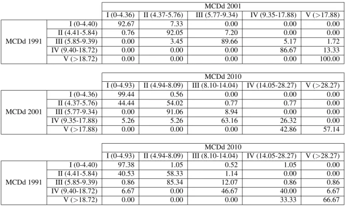
Table A.6: Transition probabilities for MCDd MCDd 2001 I (0-4.36) II (4.37-5.76) III (5.77-9.34) IV (9.35-17.88) V (>17.88) MCDd 1991 I (0-4.40) 92.67 7.33 0.00 0.00 0.00 II (4.41-5.84) 0.76 92.05 7.20 0.00 0.00 III (5.85-9.39) 0.00 3.45 89.66 5.17 1.72 IV (9.40-18.72) 0.00 0.00 0.00 86.67 13.33 V (>18.72) 0.00 0.00 0.00 0.00 100.00 MCDd 2010 I (0-4.93) II (4.94-8.09) III (8.10-14.04) IV (14.05-28.27) V (>28.27) MCDd 2001 I (0-4.36) 99.44 0.56 0.00 0.00 0.00 II (4.37-5.76) 44.44 54.02 0.77 0.77 0.00 III (5.77-9.34) 0.00 91.06 8.94 0.00 0.00 IV (9.35-17.88) 5.26 5.26 63.16 26.32 0.00 V (>17.88) 0.00 0.00 0.00 42.86 57.14 MCDd 2010 I (0-4.93) II (4.94-8.09) III (8.10-14.04) IV (14.05-28.27) V (>28.27) MCDd 1991 I (0-4.40) 97.38 1.05 0.52 1.05 0.00 II (4.41-5.84) 40.53 58.33 1.14 0.00 0.00 III (5.85-9.39) 0.86 85.34 12.07 0.86 0.86 IV (9.40-18.72) 6.67 0.00 46.67 40.00 6.67 V (>18.72) 0.00 0.00 0.00 33.33 66.67
Table A.7: Transition probabilities for ERo
ERo 2001 I (0-1.06) II (1.07-1.68) III (1.69-2.38) IV (2.39-3.20) V (>3.20) ERo 1991 I (0-0.95) 83.66 13.07 2.61 0.65 0.00 II (0.96-1.47) 21.56 61.08 12.57 4.19 0.00 III (1.48-2.10) 1.67 25.83 57.50 14.17 0.83 IV (2.11-2.95) 0.00 2.52 21.01 68.91 7.56 V (>2.95) 0.00 3.33 0.00 13.33 83.33 ERo 2010 I (0-1.37) II (1.38-2.28) III (2.29-3.43) IV (3.44-4.90) V (>4.90) ERo 2001 I (0-1.06) 88.55 8.43 1.81 1.20 0.00 II (1.07-1.68) 26.75 55.41 14.01 3.82 0.00 III (1.69-2.38) 2.52 16.81 60.50 15.13 5.04 IV (2.39-3.20) 0.00 2.70 18.02 59.46 19.82 V (>3.20) 0.00 0.00 5.56 47.22 47.22 ERo 2010 I (0-1.37) II (1.38-2.28) III (2.29-3.43) IV (3.44-4.90) V (>4.90) ERo 1991 I (0-0.95) 81.70 9.80 3.27 5.23 0.00 II (0.96-1.47) 31.74 43.11 18.56 4.79 1.80 III (1.48-2.10) 10.00 21.67 46.67 16.67 5.00 IV (2.11-2.95) 1.68 9.24 21.85 49.58 17.65 V (>2.95) 0.00 0.00 3.33 46.67 46.67