The benefits of separating early retirees from the unemployed: simulation results for Belgian wage earners

IZA DP No. 1571

The Benefits of Separating Early Retirees from

the Unemployed: Simulation Results for Belgian

Wage Earners

Raphaël Desmet

Alain Jousten

Sergio Perelman

The Benefits of Separating Early Retirees

from the Unemployed: Simulation

Results for Belgian Wage Earners

Raphaël Desmet

Federal Planning Bureau, Brussels

Alain Jousten

Université of Liège, CEPR and IZA Bonn

Sergio Perelman

University of Liège

Discussion Paper No. 1571

April 2005

Any opinions expressed here are those of the author(s) and not those of the institute. Research disseminated by IZA may include views on policy, but the institute itself takes no institutional policy positions.

The Institute for the Study of Labor (IZA) in Bonn is a local and virtual international research center and a place of communication between science, politics and business. IZA is an independent nonprofit company supported by Deutsche Post World Net. The center is associated with the University of Bonn and offers a stimulating research environment through its research networks, research support, and visitors and doctoral programs. IZA engages in (i) original and internationally competitive research in all fields of labor economics, (ii) development of policy concepts, and (iii) dissemination of research results and concepts to the interested public.

IZA Discussion Papers often represent preliminary work and are circulated to encourage discussion. Citation of such a paper should account for its provisional character. A revised version may be available directly from the author.

IZA Discussion Paper No. 1571 April 2005

ABSTRACT

The Benefits of Separating Early Retirees from the

Unemployed: Simulation Results for Belgian Wage Earners

The pool of early retirees is characterized by a large heterogeneity along several criteria. The present paper focuses on the key distinction between those in forced early retirement and those who retire early by individual choice. We start by estimating a retirement probit model for older workers in Belgium. Based on these estimates, we then perform micro-simulations relating to a hypothetical actuarial reform of a pension system, i.e., a reform imposing on average actuarial neutrality with respect to the time of retirement. We explore two scenarios, one where the entire population is subjected to the actuarial system, and one where a duly screened sub-sample of the unemployed is shielded against these actuarial adjustment factors, a group we call the truly unemployed. We evaluate the impact on the average retirement age, the pension budgets as well as indicators of redistribution within the group of the elderly. We find that the extra budgetary gain of exposing this subgroup to the full-blown reform is modest, while the distributional cost is rather high. Our results thus comfort the idea that the budgetary cost of a focused unemployment system are moderate, and that returning the unemployment insurance to its primary role might be a desirable strategy.

JEL Classification: H31, I3, J14

Keywords: retirement, older worker, inequality

Corresponding author: Alain Jousten Université de Liège Département d’Economie Boulevard du Rectorat 7, Bât. B31 4000 LIEGE BELGIUM Email: ajousten@ulg.ac.be

Financial support from FRFC (2.4544.01) is gratefully acknowledged. The authors thank seminar participants in Louvain-la-Neuve, Turin, Bonn (IZA) and Prague (CERGE-EI) for helpful comments. The ideas expressed in this paper are those of the authors, and do not necessarily reflect the position of the respective organizations, such as the Federal Planning Bureau. The first version of this paper

1. Introduction

Major demographic challenges lie ahead of the Belgian social insurance systems. Under the simultaneous effect of decreasing fertility and increasing life expectancies, pension systems all across the developed world are facing an uncertain future, Belgium being no exception to this rule. The structural weakness of these systems is their predominant pay-as-you-go structure whereby the cohort of those currently working finances the current retirees.

The Belgian social insurance system faces a simultaneous – and less universal - challenge. The marked decline in the average retirement age over the last few decades puts an additional financial burden on the systems, Belgium being among the countries with the lowest average retirement age. (see Blöndal and Scarpetta, 1998 and Dellis et al, 2004)

While the budgetary implications of the purely demographic challenges are rather well understood, the same clearly does not hold true for the overall costs of the early retirement programs. The explicit and implicit budgetary costs of early retirement programs are often hard to evaluate as they are (willingly or unwillingly) split in (unequal) fractions among a series of different actors and budgets. Against this backdrop, the literature has focused on three isolated topics. First, there is the evaluation and projection of the budgetary costs of aging and the determination of reforms to the pension system to assure its longer-run viability. The ongoing research on long-term projections of public expenditures can be seen as a prime example (Conseil Supérieur de Finances, 2004). In general, the research on the viability of pension schemes has generally remained very partial in the sense that it often neglected the explicit or implicit budgetary cost of these early retirement arrangements. Secondly, there has been a substantial and coordinated effort all across the developed world to get a better idea of the key determinants of the retirement decision (see for example Gruber and Wise, 1999 and 2004). This literature has been interested in both the demand and the supply sides of the labor market, as well as on the role that governments play on these markets. In a recent paper, Dellis et al (2004) focus their attention on the determinants of labor supply in Belgium. The authors estimate several models inspired by the methodology of Stock and Wise (1990) where rational utility maximizers choose their retirement age so as to optimize their well-being over the life-cycle. A frequent criticism of this approach challenges the key underlying assumption. Individuals are supposed free to choose the optimal retirement date from within the menu determined by retirement and early retirement programs. In the European context, this objection is particularly acute when thinking about industrial restructuring and plant closure (steel,…) as well as the transition of the countries of central and eastern Europe to market economies. A recent survey (Elchardus and Cohen, 2003) finds that more than 40 percent of Belgian male retirees have left involuntarily into retirement or early retirement, the figure being closer to 30 percent for females. Though clearly a self-reported measure, this figure is rather striking by its sheer size, as it would mean that a little less than one in two Belgian males did not have full control over his transition into retirement. It does however not mean that this decision is automatically different from the one the individual would have freely and rationally made.

Unlike the above approaches that focus on the various costs associated with the retirement systems – be it under the form of government's budgets or efficiency costs due to distortions in the labor-leisure choice – a third strand of the literature has attempted to evaluate the outcome of the social protection and pension schemes in terms of income of the elderly,

inequality and poverty (see for example Disney and Johnson, 2001 and more recently in Desmet et al, 2005).

In the present paper we unite these different approaches. Our dataset consists of a representative sample of the Belgian population aged between 50 and 64 in the mid 1990's. In our analysis, we focus our attention on the wage earners in the sample.1 We do so by exogenously splitting the population of those who leave the labor force early into two subgroups in the above-mentioned proportions. Our aim is to separate the people with a true need for insurance against the risks of disability, unemployment and collective early retirement from those who rationally opt for benefits from either of these systems. For reasons of simplicity, we call those who are involuntarily unemployed the "true" (unemployed), and by opposition those who follow individual utility maximization the "optimizers". Our analysis should be seen as a first-pass look at the question. As such, the procedure for separating the true unemployed from the optimizers should not be seen as a workable real-world alternative, but rather as a procedure to illustrate the orders of magnitude involved.

Once separated into subgroups, we analyze the retirement decision of all these individuals using the micro-estimation approach of Dellis et al (2004) to derive parameters describing their sensitivity to key social policy parameters. The basic aim we pursue is to propose a method for separating these two sub-groups by dissuading those who simply optimize into the systems. We therefore expose the entire population or a subgroup thereof to a parametric reform of the Belgian social insurance system and evaluate the budgetary impact and some measures of the distributional incidence.

The structure of the paper is as follows. Section 2 describes the general institutional setting of the Belgian social insurance regime with a special focus on wage earners. In section 3 we describe the data and the estimation strategy of our retirement model allowing for the population of early retirees to be split into true unemployed and optimizers. Section 4 contains the results of the micro-estimations. Section 5 documents the results of two simulation exercises from a budgetary and a distributional point of view. Section 6 concludes the paper.

2. Institutional settings

Belgium is characterized by the presence of several retirement income programs. Public social security programs still account for a dominant share of pension income of the elderly. Private programs, though very small in size, are the segment that experiences the strongest growth. In the past, so-called second pillar private pension schemes have essentially been confined to the higher-income workers as well as the self-employed. The segment is however expected to growth steadily in the near future because of legislation enacted in the year 2002 expanding the array of eligible products and the tax-favored nature of second pillar pension plans.2 Third pillar individual retirement arrangements take multiple forms. They range from the tax-favored individual pension savings accounts with a maximum annual contribution of EUR

1

Two motivations underlie our decision to focus our analysis on wage earners. A first reason is institutional, as wage earners are the only group of the population that is eligible for unemployment benefits. A second reasons is data availability, as the set of information available on wage earners is by far the richest in the Belgian context.

2 _{The new plans are essentially geared towards private sector wage earners. The details of the pension plan are}

linked to the industry as well that the company that the worker is affiliated with. The precise details of these pension arrangements, such as the degree of solidarity between workers, as well as the size of the contributions are negotiated between the workers and the employers at the level of the company and/or the industry.

600 per person (in the year 2003) or under the form of more traditional savings vehicles such as the tax-favored savings accounts, investments in trust funds, life insurance, etc.

The public retirement income system consists of four segments. The three main programs are essentially organized on a sectoral basis and are Bismarckian in nature. There is one social security program for the public sector, one for the private sector wage earners and one for the self-employed. The fourth component of the public system is a means-tested element that pays out a minimum benefit on the basis of need.

The wage earner’s pension scheme we focus on is by far the largest one according to the number of people affiliated with the program. It is also the largest scheme in terms of the total annual amount of contributions and benefits payments. The normal retirement age is fixed at 65 while early retirement is possible as of age 60. The program does not impose any actuarial adjustment for early claiming of benefits. However, most workers will actually be characterized by age-of-retirement-dependent social security benefits because of an incomplete career adjustment. The reason for this is that to have a full earnings history, workers have to have accumulated 45 years in insured status. Benefits are adjusted for incomplete career length, and a dropout year provision applies for those with a career that is longer than 45 years. The said standard of a normal retirement age of 65 with a 45-year career is at present only fully applicable to male workers. Women are in a transitory regime that progressively shifts the complete career standard from 40 to 45 years and the normal retirement age from 60 to 65 by the year 2009. Hence, for most women included in our analysis, normal retirement is still set at the age of 60 with a full-career length of 40 years. Benefits are computed based on the earnings during periods of affiliation with the scheme. The benefit formula, which is subject to floors and ceilings, can be represented as follows: Gross Benefit = k * Min(n,N)/N * average wage

where n represents the number of years of affiliation with the wage earner’s scheme, N the number of years required for a full career, thus ranging from 40 to 45 years depending on the sex and year of birth of the insured worker. k is a replacement rate that takes the value of 0.6 or 0.75 depending on whether the social security recipient claims benefits as a single or as a household. The variable “average wage” corresponds to gross average indexed wages at the time of retirement. Past earnings are indexed using the evolution of the consumer price index combined with occasional additional discretionary adjustments for the evolution of growth (particularly for earnings going back to the 1960's and 1970's). Periods of the life spent on replacement income (unemployment benefits, disability benefits, workers compensation…) have a double effect on benefits. First, they count towards completing the earnings history by adding additional years of earnings to the workers earnings history, hence increasing the variable n. Second, they also affect the computation of the average wage variable. Time spent on retirement income also enters the average wage formula by means of fictive earnings. Fictive earnings correspond to the extrapolation of a worker's last earnings prior to joining the social insurance program. Fictive earnings are shielded against inflation and hence imply a constant real earnings profile entering the pensions formula for time spent on replacement income. It is important to notice that these fictive earnings do not correspond to the benefit payouts under the various schemes that may sometimes be considerably different.

Once retired, retired wage earners are also shielded against inflation through an automatic consumer price index (CPI) adjustment and are subject to an earnings test. New legislation

passed in 2002 increased the earnings limits by half hence increasing incentives for individuals to continue working after claiming benefits. Currently, the earnings limit is approximately EUR 10,845 (respectively EUR 7,422) per year above (respectively below) the normal retirement age. When earning more than these thresholds, pension entitlements are completely suspended until earnings drop back below the limits. Benefits are also paid to surviving spouses, or more generally surviving dependents of deceased wage earners.

The wage-earners system is mainly financed through payroll taxes that are levied both on the side of the employers and of the employees, with a combined tax rate of 16.36 percent (no earnings limit). However, the system also receives a subsidy from the general budget of the Belgian federal government that corresponds to approximately 11 percent of overall benefit payouts.

Next to the wage-earner pension system, several other pathways into retirement have progressively evolved, particularly in the 1980's and 1990's. These alternative routes essentially aim at making retirement possible before the earliest retirement age of the wage-earner social security scheme. These early retirement schemes can be classified into two subgroups, mandatory collective early retirement schemes and individual early retirement arrangements. Notice that both ultimately lead into the social security system at the latest at the normal retirement age. All mandatory early retirement schemes are based on collective agreements between employers and employees, sometimes at the industry level, sometimes at the level of the company or even a single production site of a company. Early retirement ages as low as the age of 50 are not rare when the company is facing severe economic problems and needs to shed workers to restructure. These programs usually require the agreement of the federal government as it pays for a fair chunk of the early retirement benefits, be it through the unemployment insurance program or some other federal budget.

Individual early retirement differentiates itself from its collective counterpart by the fact that it is based on an individual’s decision to retire from work. During the years analyzed in our sample, the most prevalent individual pathway into retirement is the unemployment insurance system, which does not impose any time limit on benefit recipience.3 The system is characterized by a total lack of experience rating. Workers desiring to retire could thus ask their employer to lay them off, without any financial cost to any of the parties involved. Similarly, employers could use the system to shed older more expensive workers and retain younger cheaper and more flexible workers.

A special unemployment regime exists for a category of people called the ‘aged unemployed’. Until June 2002, unemployed aged 50 or more were automatically considered belonging to this category. The aged unemployed are essentially no longer subject to show up at the unemployment office on a regular basis or to actively look for work. Human resource managers discovered it as a perfect tool for terminating an individual employment relation at low cost to the employer. The technique, called "Canady Dry" pensions in the Belgian context, has dramatically reinforced the role of the unemployment insurance system as an early retirement route.4 The arrangement consists in the worker and his employer agreeing to have the employer lay off the worker. The latter thus becomes eligible for unemployment insurance payments within the framework of the aged-unemployed rules, hence with no

3 _{Disability insurance is not a major route towards early retirement due to rather stringent qualifying conditions}

and rather advanced screening.

4

The name is an allusion to an advertisement for the soft drink "Canada Dry", which its sparkling and slightly bitter taste resembles an alcoholic beverage, but is none. On this issue, see OECD, 2003.

obligation to look for work or pay social insurance contributions, such as pension contributions. At the same time, he does not loose any entitlement to his future pension within the regular retirement regime of the wage-earners as time spent on unemployment insurance counts fully towards the pension, just the same way as if the person would have continued to work. To make the transaction worthwhile for the worker, he either gets a lump-sum payment or an annuity payment on behalf of the employer. Formally, this payment does not correspond to a pension entitlement though it admittedly looks and acts like one.

The system of the 'aged unemployed' was reformed in July 2002 – at least in part because of the surge of Canady Dry pension arrangements. The reform tightens the rules for new entrants to the unemployment system. The minimum age for a full waiver of obligations under the unemployment insurance system was raised from 50 to 56. A new system of "mini-waiver" was introduced on the periodic visits to the unemployment insurance as of age 50, but the person still needs to be ready to accept a job.

3. Data and estimation strategy

The dataset is identical to the one used by Dellis et al (2004) for their micro-estimation exercise. The summary statistics of the sample can be found in table 1 that is taken from the above-mentioned paper. The data stem from five sources, which are mostly of administrative origin. The data were matched and merged using individuals' national identification numbers. The dataset is extremely rich as it includes data from multiple sources for a representative fraction of the Belgian population in the years 1993, 1994 and 1995. The first component of the data is the SFR (Statistiques Fiscales des Revenus) information that is collected by the Finance Ministry. It records, all information relevant for the computation of every individual’s tax liabilities. A second component is the CIP (Comptes Individuels de Pension) that is collected by the wage-earners pension administration (ONP) since the mid 50's. It includes all career information relevant for the wage-earner pension computation: gross wages, days of work, days on social insurance programs, … Other data sources include data from the self-employed social insurance administration, the civil servant pension administration, and the 1991 Census. Dellis et al (2004) used a multi-step sample selection procedure to obtain a sample of households where at least one member of the household is in the 50-64-age bracket and has not yet retired. A total of 21,818 households were used to analyze retirement decisions of men and women separately.

Table 1: Summary Statistics (TO BE UPDATED SHORTLY – ONLY SLIGHT CHANGES)

Summary Statistics Males Females

(Std) (Std) Observations Number 23,238 9,707 Retired (%) 8.6 9.9 Age Mean 54.9 (3.7) 54.2 (3.5) Married (%) 80.6 66.1 Inactive Spouse (%) 66.4 30.7

Age Difference Mean 2.7 (4.0) -1.9 (3.9)

Earnings Mean 24,017 (19,758) 15,252 (11,901)

Spouse's Earnings Mean 6,163 (9,990) 19,865 (14,004)

Life Earnings (Wage-Earners) 33,207 (12,540) 18,610 (9,238)

Males Females Sample characteristics

Number Retiring within the

next year (%) Number

Retiring within the next year (%) Age structure

50-54 11,938 3.1 5,664 5.3

55-59 8,200 9.8 3,149 9.0

60-65 3,100 26.3 894 41.3

Social Security Program

Wage-Earner 13,135 9.6 5,242 11.0 Self-Employed 3,984 5.0 1,080 7.5 Civil Servant 6,119 8.6 3,385 8.8 Region Brussels 1,850 9.1 1,330 8.7 Flanders 14,715 8.6 5,197 10.4 Wallonia 6,673 8.4 3,180 9.4

Note: Observations correspond to person-year cells; retired people are those who have (early) retirement income and have income from work smaller than a threshold of approx. EUR 7,500.

Source: Dellis et al (2004)

To determine which factors influence the retirement decision of Belgian workers, we proceed to the estimation of a retirement probit model. In line with Dellis et al (2004), we introduce financial incentive variables among the right hand side variables determining the probability to retire from the active population. A first indicator is the concept of social security wealth (SSW), which is the present discounted value of all future benefit flows from the social security system. Discounting is done allowing both for time preference and mortality adjustments. Mortality adjustments are based on education-specific life-tables as computed by Deboosere and Gadeyne (2000) based on the 1991 Census and population registers. Depending on the household situation and the system, SSW also includes an element that is a function of dependent or survivor benefits. Further the SSW measure integrates payments originating in other retirement income systems. In the Belgian context, it is not infrequent to observe individuals collecting benefits from two or three of the main pension systems. We apply the official rules that exist for cumulating benefits from the three main public systems. SSW also allows for the possibility that people exit through different pathways into retirement. Depending on the system, people can first transit through unemployment, disability or early retirement systems when exiting from the labor force, and prior to entering the ranks of the retirees in one of the three main retirement systems. Hence, the SSW

indicator is a true weighted sum of discounted benefit streams in a variety of different states of nature.

The next two incentive indicators are dynamic measures. “Accrual” represents the difference between the SSW tomorrow and the SSW today. “Peak value” represents the difference between SSW at its peak and SSW today.

In contrast to Dellis et al (2004), we separate the population of those who retire from the job market through the early-retirement or the unemployment insurance scheme into two subgroups. For the first subgroup, the true unemployed, we suppose that they have very limited options on the labor market and that an exogenous process determines their labor market transitions. Once forced into early-retirement or unemployment, they are eligible for 100 percent of the early-retirement and unemployment benefits. At this stage, we would like to reemphasize that forced retirement can perfectly be fully individually rational. In fact, we interpret the survey evidence of Elchardus and Cohen (2003) claiming that more than 40 percent of Belgian males faced forced retirement as indicator that at least for a share of these forced (early-) retirees the retirement decision must also have been worthwhile; otherwise protests would have been more widespread on the streets. Put differently, nothing precludes collectively rational decisions from being individually rational. Pushing this argument to the extreme, it is theoretically possible that although 40 percent of Belgian males claim that they were forced into retirement, not a single one actually took a decision different from the one he would have individually and rationally chosen and hence that the model of Dellis et al (2004) is an appropriate representation of reality.

Other evidence however points in the direction of some level of true unemployment among the elderly workers. When looking at administrative data on unemployment, at least two strategies seemed imaginable. The first one was to look at the unemployment rate of younger cohorts that are not yet eligible for any of the early retirement arrangements. This first approach did not allow to net out cohort specific evolutions, such as different activity rates across cohorts most notably for females. The second was to look at a sample of countries characterized by less generous old-age unemployment schemes and much lower old-age unemployment, such as the Scandinavian countries (Denmark, Sweden and Norway) and the United Kingdom. The more restrictive nature of their systems makes it more unlikely that the majority of these individuals would have freely opted into the scheme if they had not been forced into unemployment by some exogenous shock. We thus decided combine the two strategies in a difference in difference approach. Using EUROSTAT data on inactivity rates, we computed the difference between the inactivity rate of the 50 to 64 year-old and the 25 to 49 year-old for all countries concerned as an indicator of cohort-specific evolutions. We then compare the average of these differences for the reference countries from the figure we derived for Belgium. The result of this computation shows that approximately 44 percent of male and 40 percent of female aged unemployment can be explained by age-specific tendencies observed in other countries, while the remainder of the unemployment and early-retirement observed in Belgium is of the optimizing kind.

The second subgroup, the optimizers, faces a much broader choice, as their retirement decision is less deterministic. When evaluating different retirement dates, individuals compute the weighted SSW over the different possible pathways into retirement available at every single age. Optimally, we would integrate information on sectors of activity, education level and geographic region in our evaluation of the probabilities to exit the labor market. Given the lack of such detailed information, we use the countrywide observed frequencies of the early

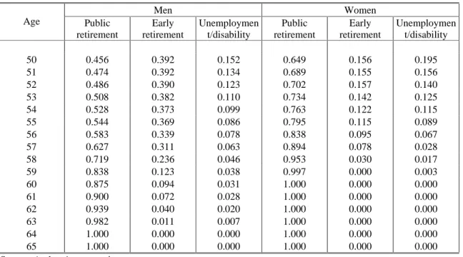
retirement and the unemployment/disability routes to determine the weights applicable to all optimizers. More specifically, the weight corresponds to the frequency of departures into the respective programs net of departures by true unemployed that follow the above-mentioned purely exogenous process (see table 2). For wage earners, we add the unemployment insurance and disability insurance paths as the two systems produce very similar benefit structures. Doing so, we give an upper bound on incentives for people to retire as we render all of disability voluntary. Given the lack of information for the public sector, we consider as early retirees all people retiring before the age of 60.

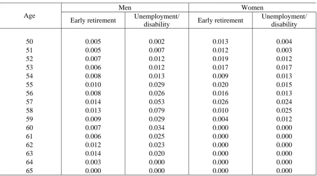
Our analysis is extreme, in the sense that we stylize people of any age cohort into two extreme subgroups, once purely passive and once totally active. To overcome the problem of deciding who is active and who is passive, we decided to expose every individual who retires within a given year to the two situations. The way we put this into practice is by "cloning" individuals who retire, while simply applying the optimizing model to all other individuals. We then allocate the probability of 44% and 40% for men and women, respectively, to the event that the person exogenously had to leave his job, and the remaining probability on the alternative state of the world. Our modelization also takes into account that every individual who currently belongs to the optimizers might one day in the future become a true unemployed and hence eligible for 100 percent of those benefits. Table 3 presents the age- and sex-specific probabilities of transition into true unemployment that we derived.

Table 2: Weight of the different pathways to retirement for optimizers (by age)

Men Women Age _Public retirement Early retirement Unemploymen t/disability Public retirement Early retirement Unemploymen t/disability 50 0.456 0.392 0.152 0.649 0.156 0.195 51 0.474 0.392 0.134 0.689 0.155 0.156 52 0.486 0.390 0.123 0.702 0.157 0.140 53 0.508 0.382 0.110 0.734 0.142 0.125 54 0.528 0.373 0.099 0.763 0.122 0.115 55 0.544 0.369 0.086 0.795 0.115 0.089 56 0.583 0.339 0.078 0.838 0.095 0.067 57 0.627 0.311 0.063 0.894 0.078 0.028 58 0.719 0.236 0.046 0.953 0.030 0.017 59 0.838 0.123 0.038 0.997 0.000 0.003 60 0.875 0.094 0.031 1.000 0.000 0.000 61 0.900 0.072 0.028 1.000 0.000 0.000 62 0.939 0.040 0.020 1.000 0.000 0.000 63 0.982 0.011 0.007 1.000 0.000 0.000 64 1.000 0.000 0.000 1.000 0.000 0.000 65 1.000 0.000 0.000 1.000 0.000 0.000 Source: Authors' computations

Table 3: Probability of forced early retirement or forced unemployment

Men Women Age

Early retirement Unemployment/

disability Early retirement

Unemployment/ disability 50 0.005 0.002 0.013 0.004 51 0.005 0.007 0.012 0.003 52 0.007 0.012 0.019 0.012 53 0.006 0.012 0.017 0.017 54 0.008 0.013 0.009 0.013 55 0.010 0.029 0.020 0.015 56 0.008 0.026 0.016 0.013 57 0.014 0.053 0.026 0.024 58 0.013 0.079 0.010 0.025 59 0.009 0.029 0.004 0.012 60 0.007 0.034 0.000 0.000 61 0.006 0.025 0.000 0.000 62 0.012 0.023 0.000 0.000 63 0.014 0.020 0.000 0.000 64 0.003 0.000 0.000 0.000 65 0.000 0.000 0.000 0.000 Source: Authors' computations

The advantage of our strategy is that we explore the available information to a maximum as we expose every single individual profile to these two scenarios. The major drawback of our approach - and of our dataset - is that we do not take into account that the probability to be forced into retirement is distributed unequally across the population, with some job profiles, and some industries being much more likely subject to an exogenous shock than others. Our strategy is not void of economic sense. Though admittedly imperfect, our approach has the advantage of recognizing the diversity within the pool of the unemployed. It is rather a first-pass analysis of the implication of applying actuarial reforms to a pool of persons that are truly unemployed or truly disabled. It should neither be seen as a truthful representation of reality, nor as a usable tool for socio-economic policy-making. The distinction between true unemployed and optimizers is hard to make in reality. In this respect, the literature on disability insurance (DI) can serve as a good guide of what is feasible, and why it is interesting to make simulations explicitly taking these subgroups into account rather than simply lumping them together. There exist an important empirical literature on the effect of DI on labor supply and retirement.5 Diamond and Mirrlees (1978, 1986) study the case of workers forced to retire early due to a disability that occurs without an observable prior signal. Truly disabled people cannot be separated from those purely claiming to be disabled. They show that the optimal DI insurance program with no cheating implies benefits rising with the age at which one starts to draw benefits, but by less than would be actuarially fair. Diamond and Sheshinski (1995) propose a model to structure optimal disability benefits in a world close to the U.S. social security system. They point out that designing optimal benefits requires a balancing of income redistribution objectives and labor supply disincentives. Faced with necessarily imperfect screening devices to determine whether a physical or mental disability translates into a labor supply problem, policy makers have different options at their hand. One is the separation of those disabilities that are easier to observe and verify (in our

5

case the "truly unemployed") into a specific system, and all other individuals into one less generous system along the lines of the Diamond-Mirrlees model.6

4. Probit estimates

We estimate a series of probit models to evaluate the impact of financial incentive variables on the probability of retirement. Our approach is one of micro-estimation as we use individual and family level data on workers to evaluate the impact of financial variables on the decision to retire, taking into account a series of control variables such as demographics and family status. The estimates allow us to get an idea of the way the Belgian social insurance system as an institution influences individual decision-making among elderly workers.

6

Table 4: Retirement Probits for Men

Accrual Peak Value

Age Age Dummies Age Age Dummies

Explanatory variables

Coef. Std.Err. Coef. Std.Err. Coef. Std.Err. Coef. Std.Err.

Intercept -8.2592 0.2743 -0.3992 0.1978 -8.1734 0.2746 -0.3251 0.1978 Incentive Measures SSW (1000’s) 0.0009 0.0003 0.0009 0.0003 0.0009 0.0003 0.0009 0.0003 Probability effect (0.0089) (0.0087) (0.0090) (0.0090) AC, PV (1000’s) -0.0426 0.0015 -0.0410 0.0016 -0.0378 0.0015 -0.0361 0.0015 Probability effect (-0.4220) (-0.3960) (-0.3689) (-0.8731) Demographic Variables Age 0.1145 0.0039 . . 0.1140 0.0039 . . Married -0.0863 0.0506 -0.0905 0.0512 -0.0828 0.0506 -0.0875 0.0512 Active Spouse -0.0651 0.0403 -0.0674 0.0408 -0.0628 0.0401 -0.0652 0.0406 Age Difference 0.0041 0.0039 0.0041 0.0040 0.0033 0.0039 0.0033 0.0040 Dependent -0.0819 0.0364 -0.0752 0.0367 -0.0855 0.0362 -0.0793 0.0365

Income Earnings Variables

Life Cycle Earnings 0.0113 0.0074 0.0125 0.0076 0.0112 0.0074 0.0124 0.0076

Earnings (1000’s) -0.0090 0.0013 -0.0092 0.0013 -0.0091 0.0013 -0.0092 0.0013

Spouse Earnings (1000’s) -0.0009 0.0025 -0.0007 0.0026 -0.0008 0.0025 -0.0007 0.0026

Age and Schemes Dummies

Age50 -2.1776 0.1154 -2.1866 0.1151 Age51 -2.1337 0.1167 -2.1536 0.1164 Age52 -1.9018 0.1128 -1.9218 0.1126 Age53 -1.8853 0.1134 -1.8806 0.1131 Age54 -1.7174 0.1122 -1.7443 0.1119 Age55 -1.5132 0.1081 -1.5358 0.1079 Age56 -1.5290 0.1093 -1.5639 0.1090 Age57 -1.3346 0.1077 -1.3580 0.1075 Age58 -1.1717 0.1081 -1.1896 0.1079 Age59 -1.4089 0.1159 -1.4657 0.1155 Age60 -0.6738 0.1062 -0.6909 0.1060 Age61 -0.6800 0.1103 -0.7020 0.1100 Age62 -1.1529 0.1211 -1.1668 0.1209 Age63 -1.0814 0.1257 -1.0985 0.1254 Age64 -1.0917 0.1350 -1.1053 0.1347 Civil Servant 0.3251 0.1405 0.3184 0.1433 0.3134 0.1413 0.3075 0.1442 Self-Employed 0.0603 0.1371 0.0735 0.1396 0.0159 0.1374 0.0286 0.1401 Pseudo R2 0.2167 0.2331 0.2094 0.2265

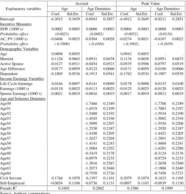
Table 5: Retirement Probits for Women

Accrual Peak Value

Age Age Dummies Age Age Dummies

Explanatory variables

Coef. Std.Err. Coef. Std.Err. Coef. Std.Err. Coef. Std.Err.

Intercept -6.3015 0.3659 -0.0943 0.2857 -6.4912 0.3649 -0.0211 0.2851 Incentive Measures SSW (1000’s) 0.0002 0.0003 0.0006 0.0003 0.0004 0.0003 0.0008 0.0003 Probability effect (0.0025) (0.0082) (0.0052) (0.0110) AC, PV (1000’s) -0.0406 0.0025 -0.0304 0.0028 -0.0274 0.0021 -0.0187 0.0022 Probability effect (-0.5800) (-0.4304) (-0.3902) (-0.2659) Demographic Variables Age 0.0898 0.0055 . . 0.0943 0.0055 . . Married 0.1126 0.0663 0.0931 0.0678 0.1176 0.0658 0.0951 0.0675 Active Spouse -0.0127 0.0511 -0.0454 0.0523 -0.0535 0.0506 -0.0797 0.0519 Age Difference 0.0177 0.0059 0.0122 0.0060 0.0171 0.0059 0.0109 0.0060 Dependent -0.1805 0.0536 -0.1913 0.0541 -0.1762 0.0534 -0.1907 0.0539

Income Earnings Variables

Life Cycle Earnings 0.0164 0.0097 0.0141 0.0099 0.0178 0.0098 0.0153 0.0100

Earnings (1000’s) -0.0118 0.0025 -0.0113 0.0025 -0.0125 0.0025 -0.0120 0.0025

Spouse Earnings (1000’s) -0.0021 0.0019 -0.0016 0.0019 -0.0017 0.0019 -0.0012 0.0019

Age and Schemes Dummies

Age50 -1.7466 0.2189 -1.7706 0.2189 Age51 -1.6519 0.2199 -1.7083 0.2197 Age52 -1.5488 0.2192 -1.5934 0.2190 Age53 -1.4545 0.2196 -1.5002 0.2194 Age54 -1.5099 0.2207 -1.5536 0.2206 Age55 -1.2530 0.2187 -1.2920 0.2187 Age56 -1.4108 0.2205 -1.4452 0.2205 Age57 -1.2637 0.2204 -1.2891 0.2203 Age58 -1.4141 0.2243 -1.4604 0.2241 Age59 -1.5604 0.2292 -1.6201 0.2286 Age60 -0.3419 0.2178 -0.3124 0.2176 Age61 -0.0979 0.2235 -0.0729 0.2233 Age62 -1.3016 0.2567 -1.2658 0.2560 Age63 -1.2073 0.2646 -1.1806 0.2640 Age64 -0.7558 0.2726 -0.7456 0.2721 Civil Servant 0.1766 0.1078 0.1397 0.1101 0.2079 0.1079 0.1623 0.1105 Self-Employed -0.0654 0.1106 -0.0736 0.1131 -0.0897 0.1103 -0.0939 0.1130 Pseudo R2 0.1692 0.2062 0.1586 0.1999

Source: Authors' computations

We estimate models using both accrual and peak value indicators for dynamic incentives, to allow for the varying time horizons that are potentially relevant for an individual's decision to retire, namely the instantaneous incentive to retire and the longer-run incentive to retire. We use two different specifications of the age variables, once linear and once under the form of dummy variables. The models with the dummy variables are presented to allow for non-linearities that our incentive measures do not fully capture. Indeed, a common feature in the retirement literature all across the world is that models based on financial incentive variables alone cannot explain the high hazard rates that we observe at key ages. Examples are the high exit rates at the earliest early retirement age as well as at the normal retirement age that cannot purely be based on financial incentives, the former being partly due to the fact that people do not think about dissociating retirement and claiming of benefits (see Coile et al, 2003) and the latter due to some peer/social pressure not to work beyond a given age. The problem with the dummy variable models is clearly identification, as it is hard or impossible to separate out

these other effect from the one due to the functioning of the (early-) retirement systems through financial incentives.

Results are presented in tables 4 and 5. Our findings are rather coherent with respect to those of Dellis et al (2004), in the sense that parameter estimates hardly vary at all. Remember that, as indicated in Section 3, the main difference between both studies relies on the way pathways to retirement and probabilities to be forced to retired are taken into account in the computation of the incentive variables (Accrual and Peak Values). The only key difference is that the sign on the SSW parameter changes from negative to positive (significant for males). This means that we now have a positive wealth effect, indicating that when people become wealthier in terms of expected benefit payouts, their probability to retire increases. This finding is more plausible than the equally significant finding of the previous authors that the wealth effect is negative and that it is only the dynamic incentive variable that influences the individual's decision in the correct direction. The estimates we find for the accrual and peak value models that comfort us in our belief that the Belgian social security system produces incentives that are all across the board biased against continued work. We interpret this as strong evidence of the pervasive effects that social protection schemes can have on individual decision-making, particularly among those that we qualify as the optimizers.

5. Simulation results

To evaluate the importance of the individual incentives, and their signification for social policy-making, we now turn to a simulation exercise. We opt for an approach of micro-simulation relying on the above data and estimates. We simulate a reform to the social protection scheme applicable to wage earners that renders it close to actuarially fair at the relevant margin, i.e. the decision to retire. More specifically, we simulate the effect of a change to the system that maintains the normal retirement age, but introduces a schedule of early retirement penalties under the form of actuarial adjustments. To determine the necessary actuarial adjustment, we turn to the evidence of Desmet and Jousten (2003) and approximate a schedule of adjustments that we apply to the wage-earner pension system (see table 6). Early retirement is allowed as early as age 50, extending the retirement window within the pension system from the current 60-65 to 50-65.

Table 6: Actuarial adjustment (unisex)

Age Actuarial Adjustment

(in %) 50 72.5 51 71.5 52 70.0 53 68.0 54 65.5 55 62.5 56 59.0 57 55.0 58 50.5 59 45.5 60 40.0 61 34.0 62 27.0 63 19.0 64 10.0 65 0.0

Source: Authors' approximations based on Desmet and Jousten (2003)

As a complement to the extension of the statutory pension system, all other early retirement routes are closed or eliminated. We simulate two different approaches, one where all early retirement possibilities are totally eliminated in a sweeping clean-up of the system. This elimination is applicable to everybody subject to the wage-earner scheme, de facto eliminating any other kind of early exit route from the labor market after age 50. This first approach (called "total") has to be seen as an interesting reference scenario, though it clearly would be hard to defend on the political scene as it totally disregards people that are exogenously pushed into early-retirement, unemployment or disability. In some sense, it tries to make people obey by the rules of optimization without having the possibility to optimize... The second approach ("partial") is less extreme and politically more plausible in the sense that it takes into account the heterogeneity in the population by only exposing the optimizers to the reform, all other individuals continuing to be protected by the specific social insurance programs (unemployment, disability and early retirement) targeted at them. The emphasis has to be put on the importance of good targeting that can only be achieved by a well-functioning control mechanism allowing these specialized programs to screen applicants. Such screening is hard to perform in reality, and we do not pretend having the miracle solution to an old and often discussed issue. We do however think that targeting of these programs more in line with their original aims can easily be improved upon. In early 2004, discussions at the level of the Belgian federal government went precisely into this direction. The employment minister suggested some stronger screening of the pool of the unemployed, notably with respect to their willingness to take up new jobs. It would have been a low-cost method of reducing the use and abuse of the system for all kinds of purposes beyond pure unemployment insurance. At the same time, he also created a grants program devoted to firms that improve the working conditions of aged, experimented, workers. As other countries, Belgium is under pressure from the European Union to rapidly improve employment rates among the 55 to 64 year-old as a key condition to face the ongoing ageing process. For the first time in many years, firms and unions accepted to discuss about ways to reform the early retirement programs. Perhaps these are the best conditions to bring down today’s perverse incentive system.

Results are presented from three different perspectives, to illustrate the ramifications of any such reform. First, table 7 presents the outcomes of the baseline situation as well as the two reform scenarios for variety of models in terms of retirement age. As suggested in Gruber and Wise (2004), three different simulation methodologies are used that differ in the way they incorporate age effects in the changes. Methodology S1 is based on the estimates of the probit models using a linear age trend, but no dummies. Methodologies S2 and S3 rely on the dummy variable models. Simulation methodology S3 distinguishes itself from simulation S2 along a single, but important margin. S3 shifts the estimated age-specific effects from the anchor-ages of the various preexisting (early-) retirement systems to the key ages of the reformed combined system. In this particular case of simulation the correct way to treat age-specific dummies is to reduce their effect by the same reduction rate as the actuarial reduction rates presented in table 6. S2, on the other hand, leaves the dummy effects unchanged at the original anchor-ages.

Table 8 presents the information of table 7 in variations. The results indicate that male wage-earners increase their retirement age by an average of 1,6 to 4,7 years when implementing the reform for all individuals. The average impact is lower by approximately half a year when limiting the reform to the optimizers. This difference of half a year might at first look like very small. However, when focusing on the truly unemployed that we protect in the partial reform, we see that changes are very dramatic in their case, ranging from two months for the partial reform to a whopping increase of almost 8 years of the average retirement age. Our results indicate that it is important not to focus on the average retirement age in the country, such as illustrated by our figures in the columns relative to the complete sample but rather focus on the subgroups subject to the reform proposals.

Table 7: Average Retirement Age

Complete Sample (23326 men and 10579 women)

Wage-Earners Only (13112 men and 5611 women)

Protected Individuals and Spouses (500 men and 209 women)

Simulated Reform Simulated Reform Simulated Reform

Model Simulation

Method Baseline

Predicted Partial Total

Baseline

Predicted Partial Total

Baseline

Predicted Partial Total

Men S1 58.57 59.33 59.58 57.87 59.01 59.45 54.02 54.21 59.10 S2 58.48 59.28 59.52 57.74 58.95 59.37 54.09 54.28 59.04 Accrual (AC) S3 58.48 60.79 60.97 57.74 61.34 62.25 54.09 54.35 62.01 S1 58.57 59.66 59.91 57.88 59.56 60.04 54.33 54.55 59.59 S2 58.52 59.65 59.90 57.78 59.54 59.99 54.42 54.64 59.57 Peak Value (PV) S3 58.52 60.93 61.09 57.78 61.58 62.47 54.42 54.71 62.22 Women S1 57.20 57.69 57.77 56.69 57.41 57.56 54.29 54.43 57.15 S2 57.27 57.71 57.78 56.83 57.49 57.61 54.74 54.90 57.12 Accrual (AC) S3 57.27 59.15 59.28 56.83 60.33 60.63 54.74 55.33 59.95 S1 57.17 57.86 57.94 56.66 57.69 57.82 54.77 54.91 57.37 S2 57.24 57.84 57.90 56.80 57.70 57.80 55.22 55.37 57.29 Peak Value (PV) S3 57.24 59.20 59.31 56.80 60.40 60.66 55.22 55.83 60.01

Table 8 : Average Retirement Age – Variation Relative to Baseline (in years) Complete Sample

(23326 men and 10579 women)

Wage-Earners Only (13112 men and 5611 women)

Protected Individuals and Spouses (500 men and 209 women)

Simulated Reform Simulated Reform Simulated Reform

Model Simulation

Method _Baseline

Predicted Partial Total

Baseline

Predicted Partial Total

Baseline

Predicted Partial Total

Men S1 58.57 + 0.76 + 1.01 57.87 + 1.14 + 1.58 54.02 + 0.19 + 5.08 S2 58.48 + 0.80 + 1.04 57.74 + 1.21 + 1.63 54.09 + 0.19 + 4.95 Accrual (AC) S3 58.48 + 2.31 + 2.49 57.74 + 3.60 + 4.51 54.09 + 0.26 + 7.92 S1 58.57 + 1.09 + 1.34 57.88 + 1.68 + 2.16 54.33 + 0.22 + 5.26 S2 58.52 + 1.13 + 1.38 57.78 + 1.76 + 2.21 54.42 + 0.22 + 5.15 Peak Value (PV) S3 58.52 + 2.41 + 2.57 57.78 + 3.80 + 4.69 54.42 + 0.29 + 7.80 Women S1 57.20 + 0.49 + 0.57 56.69 + 0.72 + 0.87 54.29 + 0.14 + 2.86 S2 57.27 + 0.44 + 0.51 56.83 + 0.66 + 0.78 54.74 + 0.16 + 2.38 Accrual (AC) S3 57.27 + 1.88 + 2.01 56.83 + 3.50 + 3.80 54.74 + 0.59 + 5.21 S1 57.17 + 0.69 + 0.77 56.66 + 1.03 + 1.16 54.77 + 0.14 + 2.60 S2 57.24 + 0.60 + 0.66 56.80 + 0.90 + 1.00 55.22 + 0.15 + 2.07 Peak Value (PV) S3 57.24 + 1.96 + 2.07 56.80 + 3.60 + 3.86 55.22 + 0.61 + 4.79

A second type of results relates to the budgetary impact of these reforms. While age-of– retirement statistics give a good indication of the individual incentives to retire, they provide absolutely no guideline as to which budgetary impact they imply for the social insurance programs and the fiscal revenues in general. Along the lines of Desmet et al (2005) we evaluate the budgetary impact for a single age-of-birth cohort of 50 year-olds in 1993, 1994 or 1995.7 Table 9 summarizes these findings both in present discounted value terms, as in relative terms. Our results indicate that the major part of the cost savings implied by our reforms occur under the form of reduced benefit flows. However, more than 20 percent of the sum of savings originates outside of the social insurance system in the fiscal departments of the government, be it through increased VAT payments on purchases or on additional payroll (social insurance) and income taxes on additional wage income during a prolonged working-life. Our results indicate that savings of these two approaches to pension reform are substantial, and that the total reform dominates the partial one from a purely budgetary perspective.

The third and last dimension we are interested in is the distributional side of any such reform proposal. In the present paper, we adopt a simplified, and maybe simplistic approach to the problem. To evaluate the distributional aspect of the problem, we turn to indicators of income inequality and poverty in the population at large, as well as for our subgroup of truly unemployed and protected individuals. These indicators are based on the lifetime income that is computed from age 50 until the end of life. It is obtained in the same way as present discounted values in table 9. Table 10 summarizes some key indicators. The change of the Gini coefficient across scenarios indicates that the strongest increase in inequality does not come from the actuarial nature of the reform in itself, but rather from the fact that the truly unemployed individuals are no longer protected from this actuarial reform. Hence, we have to conclude that it is essentially the truly unemployed that would bear the burden of the reform, as they are the ones that would suffer the biggest expected income loss of the population. Poverty rates as measured by the fraction of households with lifetime income below 50% of the average lifetime income also vary a lot across scenarios. Here, in contrast to the Gini indicator, we observe the strongest effect on the level of actuarial reform rather than on the fact of protecting the truly unemployed. Though the smallness might look surprising at first, it is actually rather plausible. Indeed, we observe that the subgroup of the truly unemployed faces a dramatically increased poverty rate when their protected status is taken away. On aggregate, this effect is much less noticed as the dramatic change in the poverty rate is only applicable to a small subgroup of the total population that suffers a lot from the reform, both in terms of average retirement age as in benefit levels. Hence, our results indicate that the social and redistributive costs of applying a total rather than a partial reform are likely to be enormous. In a cost-benefit spirit, this result has to be opposed to the difference in budgetary costs across scenarios. Our results of table 9 and 10 indicate that a total budgetary cost equivalent to some 2 to 3 percent of the expected flow of benefits could reduce the increase in inequality among the population as measured by the Gini coefficient by half.

A full evaluation of the distributional aspects is well beyond the objectives of the present paper, as it would need a refined evaluation of the labor-leisure tradeoff along the option value approach. Given the heterogeneity in the population, a complete evaluation of the change in inequality would even necessitate a way of evaluating the relative value of leisure and labor of individuals respectively belonging to the truly unemployed and the optimizers.

7

20 Table 9: Total Fiscal Impact of Reform (in Eur per worker)

PDV Total Changes Relative to Base Savings

Simulated reform Simulated reform Simulated reform

Benefits and taxes

Baseline

Partial Total Partial Total Partial Total Accrual – S1 Benefits 146,930 128,098 126,021 - 12.8% - 14.2% 18,831 20,908 Taxes : Payroll 58,716 62,459 63,225 6.4% 7.7% 3,743 4,508 Taxes : Income 81,885 83,361 83,884 1.8% 2.4% 1,476 1,999 Taxes : VAT 19,391 19,086 18,980 - 1.6% - 2.1% - 306 - 411 Sum of Savings 23,744 27,004 Accrual – S2 Benefits 147,834 128,391 126,310 - 13.2% - 14.6% 19,443 21,524 Taxes : Payroll 57,979 61,560 62,285 6.2% 7.4% 3,580 4,306 Taxes : Income 80,964 82,289 82,774 1.6% 2.2% 1,325 1,810 Taxes : VAT 19,366 19,029 18,921 - 1.7% - 2.3% - 336 - 445 Sum of Savings 24,012 27,195 Accrual – S3 Benefits 147,834 130,737 128,803 - 11.6% - 12.9% 17,097 19,031 Taxes : Payroll 57,979 68,330 69,482 17.9% 19.8% 10,351 11,503 Taxes : Income 80,964 88,321 89,168 9.1% 10.1% 7,357 8,204 Taxes : VAT 19,366 19,458 19,379 0.5% 0.1% 92 13 Sum of Savings 34,897 38,751 Peak Value – S1 Benefits 147,073 130,312 128,369 - 11.4% - 12.7% 16,761 18,704 Taxes : Payroll 58,538 66,488 67,490 13.6% 15.3% 7,951 8,952 Taxes : Income 81,713 87,261 88,000 6.8% 7.7% 5,548 6,287 Taxes : VAT 20,347 19,899 19,817 - 2.2% - 2.6% - 448 - 530 Sum of Savings 29,812 33,413 Peak Value – S2 Benefits 147,915 130,837 128,901 - 11.5% - 12.9% 17,078 19,014 Taxes : Payroll 57,896 65,626 66,586 13.4% 15.0% 7,730 8,691 Taxes : Income 80,909 86,330 87,033 6.7% 7.6% 5,421 6,124 Taxes : VAT 20,324 19,834 19,748 - 2.4% -2.8% - 489 - 575 Sum of Savings 29,740 33,254 Peak Value – S3 Benefits 147,915 131,918 130,059 - 10.8% - 12.1% 15,997 17,856 Taxes : Payroll 57,896 69,765 71,007 20.5% 22.6% 11,869 13,111 Taxes : Income 80,909 89,791 90,720 11.0% 12.1% 8,882 9,811 Taxes : VAT 20,324 20,283 20,229 - 0.2% - 0.5% - 40 - 95 Sum of Savings 36,708 40,683

Table 10: Gini indexes and poverty rates

Simulated Reform

Gini indexes and poverty rates Baseline

Partial Total Accrual – S1

Gini index 0.2366 0.2477 0.2628

Overall poverty rate 7.03 8.71 8.99

Poverty rate (protected individuals) 2.99 11.41

Accrual – S2

Gini index 0.2284 0.2451 0.2612

Overall poverty rate 6.98 9.37 9.67

Poverty rate (protected individuals) 3.13 12.27

Accrual – S3

Gini index 0.2284 0.2300 0.2477

Overall poverty rate 6.98 6.33 6.45

Poverty rate (protected individuals) 3.09 6.68

Peak Value – S1

Gini index 0.2369 0.2415 0.2601

Overall poverty rate 6.90 7.59 7.79

Poverty rate (protected individuals) 3.17 9.10

Peak Value – S2

Gini index 0.2286 0.2393 0.2590

Overall poverty rate 6.98 8.48 8.71

Poverty rate (protected individuals) 3.16 10.18

Peak Value – S3

Gini index 0.2286 0.2270 0.2448

Overall poverty rate 6.96 6.05 6.14

Poverty rate (protected individuals) 3.30 6.09

6. Conclusions

The analysis shows the large potential budgetary impact of various hypothetical reforms. These reforms, though clearly selected for comparative and illustrative purposes, illustrate the importance of behavioral effects that the citizens display when faced with a varying landscape in terms of the social insurance architecture. Different real-life reform alternatives are imaginable in the Belgian context. Any such real-life alternative will have to include – at least to some degree – some elements analyzed in our stylized scenarios, for example, changes in the key retirement ages or the use of actuarial adjustment factors, while at the same time not forgetting the labor demand side. Our full-blown reform admittedly looks somewhat unrealistic. In that sense, our partial reform is a first step in the direction of getting these hypothetical simulations closer to the field. The results indicate that even such a partial reform might have important consequences, not only in levels but also on the distributional side. The results of the present distributional analysis also illustrate the need to refine the analysis in future research.

However, we have to insist that our analysis relies - like all long-run cost projections – on some assumptions we made, most notably the limitation to the cohort of 50 year olds as well as the steady state assumption, which both clearly limit the generality with which one can apply the above results to real-world proposals. Hence there is a clear need for further research to get reform proposals closer in line with politically feasible and economically viable alternatives over the long run.

The present paper shows that the social security system at large (i.e. including unemployment and disability insurance as well as early retirement schemes) induces Belgian workers to retire earlier than they ought to. Our reform simulations imply that we bring this comprehensive social protection package closer to actuarial fairness at the margin, be it for the entire population or only a fraction thereof.

Bibliography

Blöndal, S. and S. Scarpetta (1998), "The Retirement Decision in OECD Countries", Economics Department Working Paper No. 202, OECD, Paris.

Bound, J. (1989), "The Health and Earnings of Rejected Disability Insurance Applicants", American Economic Review 79, 482-503.

Bound, J. (1991), "The Health and Earnings of Rejected Disability Insurance Applicants: Reply", American Economic Review 81, 1427-1434.

Cohen, D. and M. Elchardus (2003), Attitude et attentes en rapport avec la fin de la carrière professionnelle, TOR Groep, VUB.

Coile, C., A. Jousten, P. Diamond and J. Gruber (2002), “Delays in claiming social security benefits”, Journal of Public Economics 84, 357-386

Conseil Supérieur de Finances (2004), Rapport Annuel du Comité d’étude sur le vieillissement, Bruxelles.

Cremer, H., J.-M. Lozachmeur and P. Pestieau (2003), " Disability, preference for leisure and retirement decision", mimeo

Dellis, A., R. Desmet, A. Jousten and S. Perelman (2004), "Micro-modelling of retirement in Belgium", in J. Gruber and D. Wise, eds., "Social Security Programs and Retirement around the world: micro-estimation", NBER and University of Chicago Press, Chicago

Desmet, R. and A. Jousten (2003), “The decision to retire: Individual heterogeneity and actuarial neutrality”, manuscrit.

Desmet, R., A. Jousten, S. Perelman and P. Pestieau (2005), “Microsimulation of social security reforms in Belgium”, in Gruber, J. and D. Wise (éds.), Social Security Programs and Retirement Around the World: Fiscal Implications, University of Chicago Press and NBER, Chicago, forthcoming.

Diamond, P. and J. Mirrlees (1978), "Social insurance with variable retirement", Journal of Public Economics 10, 295-336.

Diamond, P. and J. Mirrlees, (1986), "Payroll tax financed social insurance with variable retirement", Scandinavian Journal of Economics, 88, 25-50.

Diamond, P. and E. Sheshinski (1995), "Economic Aspects of Optimal Disability Benefits", Journal of Public Economics 57, 1-24.

Disney, R. and P. Johnson, eds. (2001), “Pension Systems And Retirement Incomes Across OECD Countries”, Edward Elgar Publishing, London

Gruber, J. and D. Wise (1999), "Social security and retirement around the world", NBER and University of Chicago Press, Chicago

Gruber, J. and D. Wise (2004), "Social security programs and retirement around the world: micro-estimation", NBER and University of Chicago Press, Chicago

Institut National de Statistique (1995-1996), " Enquête sur les budgets des ménages", Bruxelles

Jousten, A. and P. Pestieau (2000), “Labor mobility, redistributon and pension reform in Europe”, forthcoming in Feldstein and Siebert, Coping with the pension crisis – where does Europe stand?, NBER and Chicago University Press, Chicago

OECD (1994), OECD Economic Survey: Belgium, Luxembourg, OECD, Paris

OECD (2003), “Vieillissement et politiques de l'emploi / Ageing and Employment Policies – Belgique”, OECD, Paris

Parsons, D. (1991), "The Health and Earnings of Rejected Disability Insurance Applicants: Comment", American Economic Review 81, 1419-1426.

Pestieau, P. and J.-P. Stijns (1999), “Social Security and retirement in Belgium”, in Gruber and Wise (1999), Social Security and retirement around the world, NBER and Chicago University Press, Chicago, 37-71.

Sneesens, H., F. Shadman and O. Pierrard (2002), “Effets des préretraites sur l'emploi”, in CIFoP (2002), “Départs à la retraite et sécurité sociale”, CIFoP, Charleroi

Stock, J. and D. Wise (1990), “Pensions, the option value of work, and retirement”, Econometrica, 58(5), 1151-1180