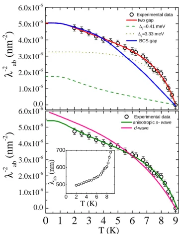
Temperature dependence of the lower critical field Hc1(T) evidences nodeless superconductivity in FeSe

Different mechanisms could take place during dust storms to shift the dust particle distribution towards a larger effective radius: (1) the lifted particle size at the surface

Importantly, expression of a cytoplasmic-targeted form of Chk1 restored DNA damage-stimulated hnRNPA0-Gadd45a mRNA binding and Gadd45a protein expression in MK2-depleted cells (

In order to study the nature of the reentrant superconducti- vity in ErRh4B4, we recently measured the variations of the superconducting critical temperature Tc, the

Separately [5], we have considered the scaling p r o p erties of the field-dependent specific heat in some detail and argued that the increase in the peak amplitude in figure 3

In the con- text of the problem of source localization, one can see three contributions: (1) propose new efficient algorithms/estimators [9], (2) study the estimation

extension of our characterization of the SmA-SmC * transition of DOBAMBC, here we will report our electrical critical field measurements in the chiral- smectic-C

The magnetization measurements where performed on an automatic pulsed field magnetometer with a maximum field of 25 T and a pulse duration of 5 ms in the temperature range of 4.2

Hysteresis loops observed on the oscilloscope screen before and after longitudinal E || (instantaneous reaction, not permanent effect) and transverse E ⊥ (gradual