Full Terms & Conditions of access and use can be found at
https://www.tandfonline.com/action/journalInformation?journalCode=thsj20
Hydrological Sciences Journal
ISSN: 0262-6667 (Print) 2150-3435 (Online) Journal homepage: https://www.tandfonline.com/loi/thsj20
Groundwater level simulation using gene
expression programming and M5 model tree
combined with wavelet transform
Ramin Bahmani, Abazar Solgi & Taha B.M.J. Ouarda
To cite this article: Ramin Bahmani, Abazar Solgi & Taha B.M.J. Ouarda (2020): Groundwater level simulation using gene expression programming and M5 model tree combined with wavelet transform, Hydrological Sciences Journal, DOI: 10.1080/02626667.2020.1749762
To link to this article: https://doi.org/10.1080/02626667.2020.1749762
Accepted author version posted online: 07 Apr 2020.
Submit your article to this journal
Article views: 12
View related articles
Publisher: Taylor & Francis & IAHS Journal: Hydrological Sciences Journal DOI: 10.1080/02626667.2020.1749762
Groundwater level simulation using gene expression programming and M5 model tree combined with wavelet transform
Ramin Bahmani1*, Abazar Solgi2, and Taha B.M.J. Ouarda1
Abstract
In order to understand and adequately manage hydrological stress, it is necessary to simulate groundwater levels accurately. In this research, gene expression programming (GEP) and M5 model tree (M5) are used to simulate monthly groundwater levels. The models are combined with wavelet transform to produce two hybrid models: wavelet gene expression programming (WGEP) and wavelet M5 model tree (WM5). For the simulation, groundwater level, temperature and precipitation values from three observation wells and one meteorological station, located in Iran, are used. The results indicate that the hybrid models, WGEP and WM5, lead to a better performance than the simple models, GEP and M5. The performance of the two hybrid models is similar. It is also observed that selecting a suitable time lag for inputs plays an important role in the accuracy of the simple models. The selection of a suitable decomposition level strongly affects the accuracy of hybrid models.
Keywords groundwater level; gene expression programming; hybrid model; M5 model tree; wavelet transform
1 Canada Research Chair in Statistical Hydro-climatology, INRS-ETE, Québec (Québec), Canada.
2 Shahid Chamran University of Ahvaz, Faculty of Water Sciences Eng., Dept. of Water Resources Engineering,
Ahvaz, Iran.
* Corresponding author: [email protected]; [email protected]
1 Introduction
Observing groundwater levels, using observation wells, is one of the main resources for investigating hydrological stresses and is necessary to understand groundwater fluctuations in arid and semi-arid areas (Ebrahimi and Rajaee, 2017, Barzegar et al., 2017). The investigation of groundwater levels provides key information to managers for decision making during extreme conditions such as during droughts (Reghunath et al., 2005, Barzegar et al., 2017).
To simulate groundwater levels, physical and mathematical models have been considered by a number of researchers. Although these models have been widely used, they have not always provided all required information concerning groundwater level simulation (Bierkens, 1998,
Nayak et al., 2006). Physical models require much more high-accuracy data for simulating groundwater levels and do not always lead to good performance in establishing non-linear relationships between variables (Nayak et al., 2006, Shiri et al., 2013). Mathematical models may lead to complex equations that are hard to solve.
For example, Qiu et al. (2015) used a mathematical model for groundwater system simulation and found that the model can efficiently simulate the system. They employed data from 190 boreholes and 260 pumping tests for the simulation. However, they announced uncertainty because of the limitation to monitor data and the lack of access to accurate input data. Yao et al. (2015) developed a numerical model to simulate groundwater flow. They indicated that the model was useful to understand complex groundwater systems, but they were
faced with limitations, such as access to input observations and the confounding human effects on the data, to reach a better accuracy.
Rajaee et al. (2019) explained that because of the practical limitations, having access to the data or solving complex equations, artificial intelligence (AI) models have been considered for simulating groundwater levels and several studies have reported the good ability of AI-based models to simulate groundwater levels (Coppola et al., 2003, Lallahem et al., 2005, Sahoo et al., 2005, Nayak et al., 2006). Among a relatively wide range of AI models, gene expression programming (GEP), in particular, has shown a high ability to efficiently simulate groundwater levels. For instance, Shiri and Kişi (2011) investigated the ability of GEP and the adaptive neuro-fuzzy inference system (ANFIS) in forecasting water table fluctuations and found that the models have a good ability to forecast the fluctuations, with the GEP leading to better results than the ANFIS. Again, Shiri et al. (2013) simulated groundwater level fluctuations by considering the meteorological effects using GEP, support vector machine and ANFIS models. They used different combinations of precipitation, groundwater level and evaporation values for simulation and concluded that GEP leads to better performance than the other methods.
The AI models have shown good performance for simulating natural variables (Chokmani et al., 2008, Solgi et al., 2017c, Eissa et al., 2013). However, they have been criticized for being black-box models with which it is hard to understand the dynamics and the effects of different variables on the simulation output (Liao and Sun, 2010, Solomatine and Xue, 2004). Hence, transparent models, such as M5 model tree (M5), which produces explicit equations, have been proposed for simulation purposes (Raza, 2015, Keshtegar et al., 2016).
The M5 model has been successfully used for simulating hydrological variables. For instance, Liao and Sun (2010) used the improved decision tree model to predict water quality.
They found the decision tree method to be more accurate and easier to use than artificial neural networks (ANNs). They concluded that improved decision tree models, which integrate some of the ANN characteristics in the main decision tree methods, were suitable for their research field. Solomatine and Xue (2004) used M5 and ANN to compare the accuracy of models for flood forecasting. Their study reported that M5 has the same accuracy as ANNs but with a number of advantages, such as transparency, high speed of training and fast convergence. In another study, Bhattacharya and Solomatine (2005) used ANN and an M5 model to develop models of the water level-discharge relationship. They concluded that both ANN and M5 models were better than the traditional rating curve, using the same data.
In more recent research, Kisi (2015) used the least square support vector machine (LSSVM), multivariate adaptive regression splines (MARS) and M5 to analyse the model accuracy in simulating summary pan evaporation. He defined different scenarios to analyse the accuracy of the models and concluded that, when the local input and output data are used, LSSVM has the best results, whereas MARS leads to a better performance when the local input and output data are not considered. Kisi (2016) used the same models to simulate evapotranspiration and concluded that LSSVR, MARS and M5 are suitable for simulation with the local input and output, without local input, and without the local input and output values, respectively. Kisi and Parmar (2016) used the same models to simulate river water pollution and concluded that MARS and LSSVM are suitable to model river water pollution.
The literature indicates that GEP and M5 have a high ability to adequately simulate hydrological time series. However, when hydrological phenomena are highly non-stationary, AI-based models may not be able to properly simulate the hydrological time series (Nourani et al., 2014). In this case, wavelet transform (WT) can be recommended as a tool for pre-processing the
time series in order to increase the accuracy of the AI-based models (Nourani et al., 2009a, Solgi et al., 2017c). Wavelet transform helps hydrologists decompose a time signal into sub-signals, allowing the models to capture information with different resolution levels (Nourani et al., 2009b).
The WT technique was presented by Grossmann and Morlet (1984) in the field of geoscience and has been adapted for the pre-processing of time series in hydrology (Oh et al., 2017,
Ouachani et al., 2013, Shoaib et al., 2015, Sivapragasam et al., 2015, Solgi et al., 2017a). Partal and Kişi (2007) used WT to decompose daily precipitation time series to sub-signals. Then, the sub-signals were entered as inputs to a neuro-fuzzy (NF) model to forecast precipitation. They reported that, when WT was used, the NF model led to a better fit with observed values. Shoaib et al. (2015) combined GEP with WT to predict runoff and concluded that using WT improves the performance of GEP. Kisi and Shiri (2011) used GEP and NF models to forecast precipitation, and also combined the models with WT to produce hybrid models. They concluded that hybrid models were more accurate than simple models and GEP combined with WT led to the best results.
Rezaie-balf et al. (2017) applied multivariate adaptive regression splines (MARS) and M5 to simulate groundwater level fluctuations in unconfined aquifers. Then, they coupled WT with MARS and M5 in order to improve the accuracy of the models. They deduced that the models combined with WT were more accurate than their simple counterparts. Seo et al. (2015) investigated the performance of ANN and ANFIS combined with WT for daily water level forecasting in reservoirs. They found that the performance of the hybrid models was better than that of their corresponding simple modes.
To the best of the author’s knowledge, there is no study to compare the ability of GEP and M5 in combination with WT to simulate groundwater levels. The first objective of this study is to simulate monthly groundwater levels using GEP and M5. The models are also combined with WT to produce hybrid models (WGEP and WM5) for groundwater simulation. For the simulation using the simple models, different combinations of groundwater level, precipitation and temperature time series are used, while for that using the hybrid models, the time series is decomposed to sub-signals using WT. Then, the sub-signals are used as inputs to the GEP and M5 models. Finally, the performance of the simple and hybrid models is compared to evaluate their accuracy.
This paper is structured as follows. Section 2 provides a review of the theoretical background of the models used in this study, and the methodology adopted to produce the hybrid models and to compare the performance of the various models. Section 3 presents the case study. The results are presented and discussed in Section 4. Finally, the conclusions and recommendations for future work are presented in Section 5.
2 Methods
2.1 Gene expression programming (GEP)
Gene expression programming was introduced by Ferreira (2001) and is part of what is called ‘evolutionary algorithms’. Evolutionary algorithms, inspired by the Darwinian evolution theory, are algorithms that imitate the mechanism of living organisms. GEP differs from other models such as ANN, in that the structure, including the input variables, target and position function, are firstly defined. Then, the optimal structure of the model and coefficients are determined during
the training process, whereas in the ANN model, the structure must be determined and only the coefficients of the model are obtained during the training process. This helps provide more flexibility to the GEP model and generally represents an advantage. The general process of solving a problem with GEP is briefly illustrated by the following steps.
Step 1. Select a terminal set, which includes dependent and independent values. Here, the root mean square error (RMSE), as the fitness function, is used.
Step 2. Choose a set of functions which includes arithmetic operators, test functions and Boolean functions. The 10 mathematical operators used are: multiplication, division, addition, subtraction, exponential, square root, natural logarithm, x to the power of 2, cube root and inverse. The arithmetic operators of addition, subtraction and multiplication are the most common types.
Step 3. Obtain the accuracy index of the model which indicates the model ability to solve a specific problem.
Step 4. Select stopping criteria, which are measures for stopping the program and obtaining the results, such as generated numbers or the maximum fixation.
Step 5. Determine the control components, including numerical values and qualitative variables. These are used for controlling the program.
This paper does not delve into the detailed theory of GEP. For more information, the reader is referred to Ferreira (2001), Ferreira (2002), and Ferreira (2006).
2.2 M5 model tree
The M5 model tree (M5) was introduced by Quinlan (1992) based on the decision tree method. The main advantage of M5 is that it presents a set of linear regressions that show the relationships between dependent and independent variables and they are interpretable (Raza, 2015). The M5 model lies between linear models, like ARIMA, and non-linear models, like ANNs (Solomatine and Xue, 2004). M5 includes a root, branches, nodes and leaves like a tree and is drawn using a top-down approach. The root as the first node is on the top and the tree grows down by nodes and branches to reach leaves. In M5, every leaf is a linear regression. Building the M5 model involves two steps. The first step consists in building a tree using a splitting criterion. The second step consists in pruning branches and replacing them with linear regression models.
2.2.1 Splitting criterion
The splitting criterion explains the rate of errors at the node and is based on minimizing the standard deviation of nodes. Because of the splitting process, the standard deviation in a given node, called the child node, is generally smaller than the standard deviation in the previous node, called the parent node (Kisi, 2015). A node ends in a leaf when minimizing standard deviation in the node is not possible. For the calculation of the reduction in standard deviation in a given node, SDR, the following equation is used (Quinlan, 1992):
SDR = sd( ) − | || |sd( ) (1)
where T is a set of training data that reaches the parent node; Ti is a subset of the training data having the ith outcome of the potential set; and sd refers to the standard deviation (Kisi, 2015).
The M5 model selects the minimum expected error for each attribute at that node. For more details concerning the splitting criterion, the reader is referred to Quinlan (1986) and Quinlan (1992).
2.2.2 Pruning
The splitting process produces a huge tree that may cause overfits to the training data. Therefore, it is necessary to prune the branches. The recommended algorithm for pruning is the Quinlan algorithm. First, the algorithm allows the tree to grow as much as possible. Second, it prunes the branches that do not increase the accuracy of the model. Finally, after the pruning, smoothing is needed to smooth sharp dissociation (Solomatine and Xue, 2004, Bhattacharya and Solomatine, 2005). For more details concerning the general M5 model, the reader is referred to (Quinlan, 1992).
2.3 Wavelet transform
The application of the wavelet transform (WT) in the geoscience discipline was introduced by Grossmann and Morlet (1984). The WT is an effective digital signal processing technique to extract hidden information from a signal. The WT was formulated as the continuous wavelet transform (CWT) by Mallat (1989), as follows:
where f(t) is the continuous signal, ( ) is the wavelet function or mother wavelet and * refers to the complex conjugate. A mother wavelet has three characteristics: (i) a limited number of fluctuations; (ii) quick return to zero in both positive and negative directions in its domain; and (iii) zero average (Thuillard, 2001).
A mother wavelet is defined as (Oh et al., 2017):
( , )( ) = | | . − , ∈ , ∈ , ≠ 0 (3)
where a is a dilation factor, b is a temporal translation, and R is the domain of real numbers.
For practical applications, hydrologists and modellers in general often have access to discrete time signals (Nourani et al., 2014). Therefore, a discrete extension of equation (2) called ‘discrete wavelet transform’ (DWT) was proposed. The DWT is defined by (Kisi and Shiri, 2011):
DWT ( , ) = 2 ∗( 2 − ) ∙ ( ) ∙ d (4)
where f(t) is a discrete time series at any time t; and j and k are integers which respectively control the wavelet dilation and the translation.
By using high-pass and low-pass filters, Mallat (1989) developed a way to implement the DWT. In the DWT, for the first decomposition level, a signal is decomposed to an approximation (A) and detail (d). The processed approximation is then applied to consequent decompositions
2.3.1 Choice of a mother wavelet
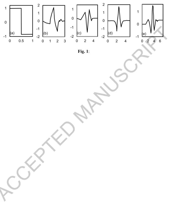
The main consideration for selecting a mother wavelet is the type of the time series. The main features of a mother wavelet include the region of support, associated with the wavelet span length, and the number of vanishing moments, limiting the ability of a wavelet to show information in a time series. In This work, the Haar, Coif1, Sym3, Db4 and Db2 wavelets, which are commonly used in hydrological studies, are adopted for decomposing time signals (Shoaib et al., 2015, Nourani et al., 2014, Solgi et al., 2017b). Figure 1 illustrates the graph of the mother wavelets..
2.4 Hybrid wavelet M5 model tree (WM5) and wavelet gene expression programming (WGEP) model development
To develop hybrid models with the wavelet transform, the following steps are carried out. The groundwater level, temperature and precipitation time series are decomposed to sub-signals using DWT for different decomposition levels. Then, the sub-signals are used as inputs into the GEP and M5 models, which are then referred to as WGEP and WM5. Figure 2 presents a schematic diagram for producing the WGEP and WM5 models. To determine the level of decomposition (L), the suggested equation of Nourani et al. (2009b) is used.
= Int[log( )] (5)
where L is the proposed decomposition level and N is the number of observed values.
2.5 Evaluation criteria
Evaluation criteria serve to estimate the errors of models according to observed and simulated values. In this paper, the following criteria are used to evaluate the models (Chebana et al., 2014): determination coefficient (R2), root mean square error (RMSE), relative root mean square error (rRMSE), mean bias (BIAS) and relative mean bias (rBIAS). The following formulae are used: = 1 −∑(∑( )) (6) RMSE = ∑( ) (7) rRMSE = 100 ∑( ) (8) BIAS = ∑( ) (9) rBIAS = 100 × (∑ ) (10)
where Hobs refers to the observed values, Hsim refers to the simulated values, is the average of observed values and n is the number of observations.
In addition to the above-mentioned evaluation criteria, the Akaike information criterion (AIC) is also considered to find the best model regarding their complexity and performance. The AIC evaluates the simulation ability of different models relative to each other (Samadianfard et al., 2018) and is calculated as follows:
AIC = × ln + 2 (11)
where K is the number of parameters of the model and RSS = ∑( − ) . A smaller value of AIC indicates a better performance of the model compared to other models.
3 Case study and data used
The methods are applied to the data of the Delfan plain, located in the north of Lorestan Province, Iran. The plain is located between 47°21 –48°21 E and 33°48 –34°22 N (see Fig. 3) at an altitude of 1700–2100 m a.s.l., and is surrounded by the Zagros Mountain chain. The plain includes three observation wells, which are just used for groundwater level and groundwater quality monitoring. Data is recorded once a month for each well.
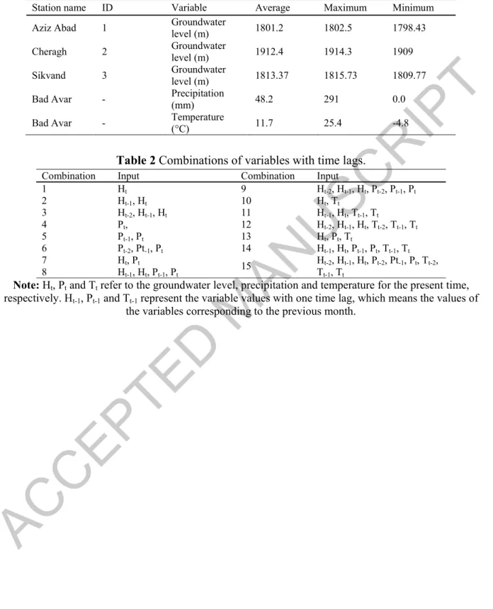
The total area of the plain is about 300 km2. The high lands of the region are formed by thick layers of limestone and the lowland areas are formed by a combination of igneous, metamorphic and calcareous structures mixed with metamorphic sheets. The morphological units of the plain consist of different alluvial structures, such as fans and debris. The average annual rainfall in the plains is 480 mm/year. Table 1 presents the features of three observation wells and one meteorological station located in the plain.
Monthly groundwater level (m), precipitation (mm) and temperature (ºC) data for the period 2002–2012 are used to simulate groundwater level one month ahead. Precipitation and temperature are selected because they both directly influence groundwater levels (Rezaie-balf et al., 2017).
In fact, air temperature may affect groundwater levels through a number of processes. First, air temperature affects water consumption. Although temperature may not affect the aquifer directly, in arid and semi-arid regions like Iran, agricultural and domestic water use rely on
groundwater and they increase or decrease according to the atmospheric temperature. Consequently, air temperature can affect groundwater fluctuations indirectly. Second, air temperature may affect evaporation in the upper layer of the soil, as well as the rate of plant transpiration, hence reducing the recharge to the aquifer from precipitation. Here again, air temperature ends up having an indirect effect on groundwater levels through its influence on evapotranspiration.
In general, groundwater level responds to the input variables with a delay. Therefore, in this paper, the input values are considered with time lags. A time lag refers to the value of a variable corresponding to previous months. Table 2 presents different combinations of variables with time lags.
For simulation purposes, the observation series, including air temperature, groundwater level and precipitation, are divided into two parts. The first part comprises 75% of the series and is used as input values to calibrate the models for simulating groundwater levels one month ahead. Then, the second part, which comprises 25% of the observation series, is employed for the validation of the models.
In Eq. (5), to produce hybrid models, L can take the value of 2. However, to investigate the effect of the decomposition level on the simulation, values of L = 1 to 4 are considered in this study.
4 Results and discussion 4.1 GEP model
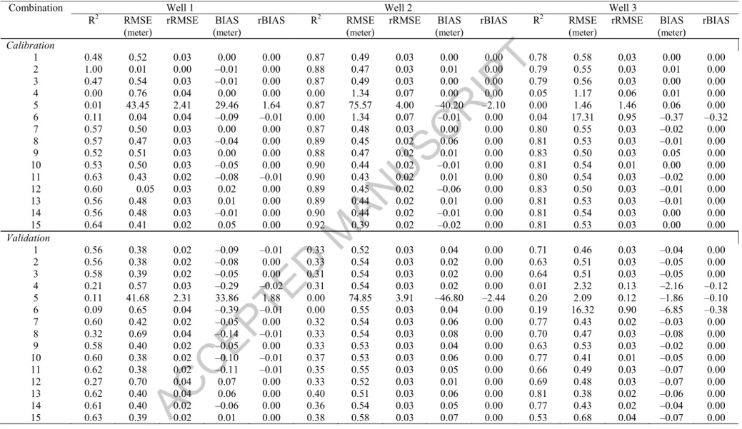
Different combinations are used for the calibration and validation of the GEP model. The results of the evaluation criteria for the calibration and validation data are presented in Table 3.
According to the results in Table 3, for Well 1, Combination 15 can be selected as the best combination for the GEP model, with the R2 is equal to 0.64 and 0.63 for the calibration and validation, respectively. For the combination, RMSE and rRMSE are small and the rBIAS value is zero which indicates that the model is unbiased. For Well 1, although the R2 of Combination 2 is equal to 1 for calibration, the combination is not selected as the best one because its R2 decreases to 0.56 for the validation.
For Well 2, GEP shows a weak performance. For calibration, most of the combinations show high R2 values and small RMSE and BIAS, whereas for validation, R2 is low and the combinations indicate large RMSE and BIAS values. For Well 2, Combination 13 is selected as the best combination.
For Well 3, Combination 13 is also selected as the best combination because it leads to a high R2 value and zero rBIAS for calibration and has the highest R2 value for validation.
According to the results, it is concluded that using variables with time lags produces more accurate results. It is important to mention that the results of the GEP model for combinations 4, 5 and 6, where just precipitation values are used, is too weak for all observation wells.
4.2 M5 model
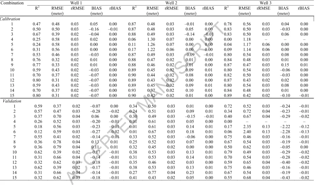
To calibrate and validate the M5 model, different combinations from Table 2 are considered as well. The results of the best combinations for calibration and validation data are presented in Table 4.
According to the results in Table 4, Combination 10 can be selected for groundwater level simulation at Well 1. The evaluation criteria of Combination 12 show better results for calibration, but it is not selected as the best model because its R2 decreases from 0.80 to 0.32 for validation, and its RMSE and BIAS increase to 0.62 and –0.18, respectively. For Well 1, combinations 10, 11 and 12 are similar to combinations 13, 14 and 15, respectively, because the M5 model does not use precipitation values in the simulation. For Well 1, M5 leads to a better performance when groundwater level and temperature values are used. On the other hand, the model shows low performances when precipitation values are considered.
For Well 2, Combination 15 can be selected as the best since it has the largest R2 value for validation. The performance of M5, likewise GEP, is not good for the groundwater level simulation of Well 2. For calibration, M5 shows high R2 and low RMSE and BIAS values, while for validation, the R2 corresponding to all combinations decreases considerably. The weak performance of the models for Well 2 may be due to the higher elevation of the well. The well is located at a higher altitude than the other wells and the mean groundwater level in Well 2 is over 1900 m a.s.l., while for wells 1 and 3 it is around 1800 m a.s.l. For Well 2, similarly to Well 1, when only precipitation data is used (combinations 4–6) the performance of the model decreases.
For Well 3, Combination 10 is selected as the best combination because it shows a high performance for both calibration and validation and it leads to similar values of R2, RMSE, rRMSE, BIAS and rBIAS for calibration and validation. Similarly to wells 1 and 2, when only precipitation data is used for the simulation, the model leads to a lower performance.
4.4 WGEP model
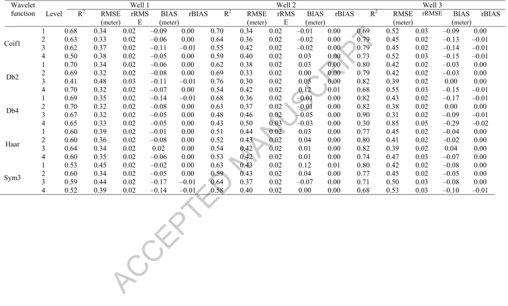
The results of the evaluation criteria for the WGEP model are shown in Table 5 for calibration, and Table 6 for validation. The esults indicate that, for Well 1, the mother wavelet of Db4, with
L = 2, can be selected as the suitable structure for simulation. For Well 1, Db2 with L = 1 and L =
4 also leads to a good performance for validation. However, these combinations are not selected because Db2 with L = 4 has an overly complex structure and for Db2 with L = 1, the R2 decreases from 0.8 in calibration to 0.7 in validation, which may indicate that the structure is not good for generalization.
The best result for Well 2 is obtained with the mother wavelet of Db2 with L = 3, for which good performance is obtained with both calibration and validation data. The best result for Well 3 is obtained with the mother wavelet of Db4 with L = 3.
The comparison of Table 4 with Tables 5 and 6 shows that using the WT improves the performance of the GEP model. The improvement is considerable for Well 2 in validation. Its R2 increases from 0.4 for the best combination to 0.76 for the best mother wavelet.
4.5 WM5 model
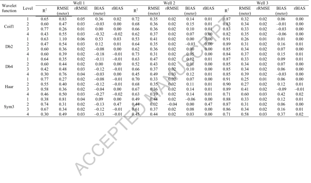
The results of the evaluation criteria for the WM5 model are presented in Table 7 for calibration and Table 8 for validation. For Well 1, the mother wavelets of Coif1 with L = 3 and Haar with L = 1 show high performance for validation. However, Coif1 with L = 3 is selected as the best mother wavelet because its R2 value is higher than Haar with L = 1 for calibration. Also, its RMSE, rRMSE, BIAS and rBIAS are smaller than Haar with L = 1.
For Well 2, Db2 with L = 4 leads to the best performance. For Well 3, all mother wavelets show good performance. However, the mother wavelet Db2 with L = 1 is selected as the best
model because the evaluation criteria for both calibration and validation are high and close to each other.
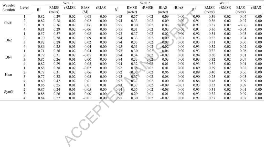
Looking at Tables 7 and 8, it can be concluded that using WT increases the accuracy of M5. Furthermore, it can be concluded that the use of a high level of decomposition does not always lead to an increase in the performance of the models. In a high decomposition level, the sub-signals are too smooth, which means that they do not carry much information. As an example, Fig. 4 presents sub-signals of temperature time series with the mother wavelet of Coif1 with L = 8. Figure 4 shows that when the decomposition level increases, the sub-signals become overly smooth.
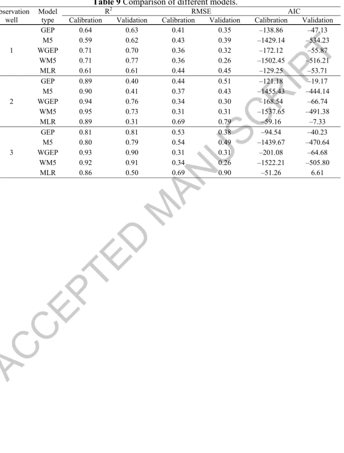
4.6 Comparison of the models studied
Table 9 presents the R2, RMSE and AIC values for the best results of the M5, GEP, WM5 and WGEP models. The rRMSE, BIAS and rBIAS values are not presented because their values are very similar and close or equal to zero.
In addition to the compression of predicted and observed values, the results are also compared to the outputs of the multiple linear regression (MLR) model, which is used as a benchmark. The MLR model is applied to the same data, used for the AI models. The results of MLR model are presented in Table 9.
The performances of M5 and GEP for different combinations indicate that precipitation is not an effective variable for simulation, unlike temperature and groundwater levels. It makes more sense to find a relation between groundwater levels and previous precipitation, because groundwater recharge depends on precipitation, and ultimately, groundwater level depends on
recharge to the aquifer. The low effect of precipitation in simulation may be explained by the fact that the case study is located in a semi-arid region where precipitation is usually zero for several months, during the end of the spring, the whole summer and the beginning of the fall. During these months, groundwater fluctuations are observed despite the fact that precipitation is continuously null. Therefore, the M5 and GEP models cannot effectively establish a relationship between precipitation and groundwater level values and this represents a weakness of the models.
According to Table 9, for all observation wells, the performance of hybrid models is better than that of simple models. In terms of R2 and RMSE, the performance of WGEP and WM5 is close and it is hard to select one of them as the best model. For Well 1, the calibration results are close, but for validation, WM5 is a little better than WGEP. For Well 2, the validation results of WGEP show better performance than WM5. Finally, for Well 3, WGEP is a little better than WM5 for both calibration and validation data, while WM5 shows a slightly better performance than WGEP.
Although the performance of both hybrid models is similar, the AIC values indicate that WM5 performs better than WGEP for simulation. A similar conclusion can be made for the comparison of GEP and M5. GEP produces complex functions to reach the best accuracy, while M5 presents the same accuracy with significantly simpler functions.
Regarding the results of the MLR model as a benchmark, the performance of the simple AI models, GEP and M5, does not show a considerable improvement in the calibration. The R2 values of GEP, M5 and MLR for Well 1 and Well 2 are similar. For Well 3, the R2 of the MLR model is better than that of the simple AI models. In terms of RMSE and AIC, the GEP and M5 models perform better than MLR for the calibration. The comparison of evaluation criteria for
validation shows that the simple AI models outperform MLR: they lead to larger R2 and smaller RMSE and AIC values than MLR. This indicates that the probability of overfitting is lower for GEP and M5 than for MLR.
The comparison of the results of the hybrid AI models, WGEP and WM5, with the MLR model as a benchmark indicates that the AI models outperform MLR for both calibration and validation. For all of the wells, the hybrid AI models lead to larger R2 and smaller RMSE and AIC values than MLR. The comparison results indicate that applying WT improves the ability of GEP and M5 models to produce appropriate groundwater level simulations.
The simulated values for the validation are presented in Fig. 5 and compared to the observed values. In Fig. 5, it can be seen that the hybrid models lead to a better fit with observations in comparison with the simple models.
5 Conclusions and future work
This paper proposes a few methods to simulate groundwater levels. The GEP and M5 models are used for the simulation and WT is used to produce hybrid models, WGEP and WM5. The MLR model is also applied to the same data and its results are used as benchmark for comparison purposes.
The results indicate that the performance of WGEP and WM5 is similar and it is shown that hybrid models are more accurate than the simple ones. Also, the comparison of the results of hybrid models with the benchmark indicates that WT improves the ability of the models for groundwater level simulation. M5 and WM5 present two advantages. First, the generated models are simpler and more interpretable. It is possible to understand which independent variables have
more effect on simulating the dependent variable. Second, running the M5 and WM5 models is faster than running the GEP and WGEP models, respectively.
Based on the results of this work, it can be concluded that first selecting a suitable lag time for input values plays an important role in groundwater level simulation. If a large number of lag times is used, the time for simulation increases, while the lag times are not always helpful to improve the accuracy. Therefore, an optimal number of lag times for input values must be identified. Second, selecting a suitable decomposition level affects the accuracy of hybrid models. A high level of decomposition is not always helpful to increase the accuracy of the model and an optimal decomposition level must also be identified.
Furthermore, it was concluded that temperature and groundwater level values are more effective variables than precipitation for groundwater level simulation in this arid region of Iran. This means that the selection of hydrological variables as inputs to the models is very specific to the region of study and the climate in question, and it affects significantly the performance of the models. Therefore, it is recommended to carry out exhaustive studies in the future in order to evaluate the effects of other hydrological variables on groundwater simulation and understand the dynamics involved, with the objective of finding suitable variables for groundwater modelling in different climates and conditions.
A good understanding and explanation of the natural phenomena involved is important. The functions produced by GEP for the modelling are too complex and it is hard to understand the relationship among variables. Functions generated by M5 are simpler, but it is still not possible to find an exact explanation of the nature of groundwater level changes based on input variables. The considered models do not seem to be able to explain the physical phenomena involved.
In this work, the simulation of groundwater levels was carried out using simple and hybrid models. It would be of interest to evaluate the ability of these models, and other models, for the long-term prediction of groundwater levels. This is important as the efficient management of a number of environmental issues (such as droughts) requires a long-term plan.
In this paper, WT was used to improve the accuracy of the models. It is also suggested, for future studies, to evaluate the effect of using other techniques, such as empirical mode decomposition (Lee and Ouarda (2011), as a tool for pre-processing hydrological time series for groundwater level simulation.
Acknowledgements
The authors wish to express their appreciation to Editor Dr. Aldo Fiori and Associate editor Corinna Abesser, and three anonymous reviewers for their invaluable comments and suggestions which helped considerably improve the quality of the paper.
Funding
This work was partially supported by the Natural Sciences and Engineering Research Council (NSERC) of Canada and the Canada Research Chair (CRC) programme.
References
Barzegar, R., Fijani, E., Asghari Moghaddam, A. & Tziritis, E. 2017. Forecasting of groundwater level fluctuations using ensemble hybrid multi-wavelet neural network-based models.
Science of The Total Environment, 599-600, 20-31.
Bhattacharya, B. & Solomatine, D. P. 2005. Neural networks and M5 model trees in modelling water level–discharge relationship. Neurocomputing, 63, 381-396.
Bierkens, M. F. P. 1998. Modeling water table fluctuations by means of a stochastic differential equation. Water Resources Research, 34, 2485-2499.
Chebana, F., Charron, C., Ouarda, T. B. M. J. & Martel, B. 2014. Regional Frequency Analysis at Ungauged Sites with the Generalized Additive Model. Journal of Hydrometeorology, 15, 2418-2428.
Chokmani, K., Ouarda, T. B. M. J., Hamilton, S., Ghedira, M. H. & Gingras, H. 2008. Comparison of ice-affected streamflow estimates computed using artificial neural networks and multiple regression techniques. Journal of Hydrology, 349, 383-396.
Coppola, E., Szidarovszky, F., Poulton, M. & Charles, E. 2003. Artificial Neural Network Approach for Predicting Transient Water Levels in a Multilayered Groundwater System under Variable State, Pumping, and Climate Conditions. Journal of Hydrologic
Engineering, 8, 348-360.
Ebrahimi, H. & Rajaee, T. 2017. Simulation of groundwater level variations using wavelet combined with neural network, linear regression and support vector machine. Global and
Planetary Change, 148, 181-191.
Eissa, Y., Marpu, P. R., Gherboudj, I., Ghedira, H., Ouarda, T. B. M. J. & Chiesa, M. 2013. Artificial neural network based model for retrieval of the direct normal, diffuse horizontal and global horizontal irradiances using SEVIRI images. Solar Energy, 89, 1-16.
Ferreira, C. 2001. Gene Expression Programming: A New Adaptive Algorithm for Solving
Problems, Angra do Heroísmo, Portugal, Complex Systems Publications.
Ferreira, C. 2002. Gene Expression Programming in Problem Solving. In: ROY, R., KÖPPEN, M., OVASKA, S., FURUHASHI, T. & HOFFMANN, F. (eds.) Soft Computing and
Industry: Recent Applications. London: Springer London.
Ferreira, C. 2006. Gene Expression Programming Mathematical Modeling by an Artificial
Intelligence, Germany, Springer-Verlag Berlin Heidelberg.
Grossmann, A. & Morlet, J. 1984. Decomposition of Hardy Functions into Square Integrable Wavelets of Constant Shape. SIAM Journal on Mathematical Analysis, 15, 723-736. Keshtegar, B., Piri, J. & Kisi, O. 2016. A nonlinear mathematical modeling of daily pan
evaporation based on conjugate gradient method. Computers and Electronics in
Agriculture, 127, 120-130.
Kisi, O. 2015. Pan evaporation modeling using least square support vector machine, multivariate adaptive regression splines and M5 model tree. Journal of Hydrology, 528, 312-320. Kisi, O. 2016. Modeling reference evapotranspiration using three different heuristic regression
approaches. Agricultural Water Management, 169, 162-172.
Kisi, O. & Parmar, K. S. 2016. Application of least square support vector machine and multivariate adaptive regression spline models in long term prediction of river water pollution. Journal of Hydrology, 534, 104-112.
Kisi, O. & Shiri, J. 2011. Precipitation Forecasting Using Wavelet-Genetic Programming and Wavelet-Neuro-Fuzzy Conjunction Models. Water Resources Management, 25, 3135-3152.
Lallahem, S., Mania, J., Hani, A. & Najjar, Y. 2005. On the use of neural networks to evaluate groundwater levels in fractured media. Journal of Hydrology, 307, 92-111.
Lee, T. & Ouarda, T. B. M. J. 2011. Prediction of climate nonstationary oscillation processes with empirical mode decomposition. Journal of Geophysical Research: Atmospheres, 116, n/a-n/a.
Liao, H. & Sun, W. 2010. Forecasting and Evaluating Water Quality of Chao Lake based on an Improved Decision Tree Method. Procedia Environmental Sciences, 2, 970-979.
Mallat, S. G. 1989. A theory for multiresolution signal decomposition: the wavelet representation. IEEE Transactions on Pattern Analysis and Machine Intelligence, 11, 674-693.
Nayak, P. C., Rao, Y. R. S. & Sudheer, K. P. 2006. Groundwater Level Forecasting in a Shallow Aquifer Using Artificial Neural Network Approach. Water Resources Management, 20, 77-90.
Nourani, V., Alami, M. T. & Aminfar, M. H. 2009a. A combined neural-wavelet model for prediction of Ligvanchai watershed precipitation. Engineering Applications of Artificial
Intelligence, 22, 466-472.
Nourani, V., Hosseini Baghanam, A., Adamowski, J. & Kisi, O. 2014. Applications of hybrid wavelet–Artificial Intelligence models in hydrology: A review. Journal of Hydrology, 514, 358-377.
Nourani, V., Komasi, M. & Mano, A. 2009b. A Multivariate ANN-Wavelet Approach for Rainfall–Runoff Modeling. Water Resources Management, 23, 2877.
Oh, Y.-Y., Yun, S.-T., Yu, S. & Hamm, S.-Y. 2017. The combined use of dynamic factor analysis and wavelet analysis to evaluate latent factors controlling complex groundwater level fluctuations in a riverside alluvial aquifer. Journal of Hydrology, 555, 938-955.
Ouachani, R., Zoubeida, B. & Taha, O. 2013. Power of teleconnection patterns on precipitation and streamflow variability of upper Medjerda Basin. International Journal of
Climatology, 33, 58-76.
Partal, T. & Kişi, Ö. 2007. Wavelet and neuro-fuzzy conjunction model for precipitation forecasting. Journal of Hydrology, 342, 199-212.
Qiu, S., Liang, X., Xiao, C., Huang, H., Fang, Z. & Lv, F. 2015. Numerical Simulation of Groundwater Flow in a River Valley Basin in Jilin Urban Area, China. Water, 7, 5768-5787.
Quinlan, J. R. 1986. Induction of decision trees. Machine Learning, 1, 81-106.
Quinlan, J. R. 1992. Learning with Continuous Classes. Proceedings of Australian Joint
Conference on Artificial Intelligence, Hobart, Australia, World Scientific, Singapore,
343-348.
Rajaee, T., Ebrahimi, H. & Nourani, V. 2019. A review of the artificial intelligence methods in groundwater level modeling. Journal of Hydrology, 572, 336-351.
Raza, K. 2015. M5 Model Tree and Gene Expression Programming for the Prediction of Metrological Parameters. Proceeding of IEEE 2015 International Conference on
Computers, Communications, and Systems (ICCCS-2015), Nov 2-3, 2015. Kanyakumari,
India.
Reghunath, R., Murthy, T. R. S. & Raghavan, B. R. 2005. Time Series Analysis to Monitor and Assess Water Resources: A Moving Average Approach. Environmental Monitoring and
Assessment, 109, 65-72.
Rezaie-Balf, M., Naganna, S. R., Ghaemi, A. & Deka, P. C. 2017. Wavelet coupled MARS and M5 Model Tree approaches for groundwater level forecasting. Journal of Hydrology, 553, 356-373.
Sahoo, G. B., Ray, C. & Wade, H. F. 2005. Pesticide prediction in ground water in North Carolina domestic wells using artificial neural networks. Ecological Modelling, 183, 29-46.
Samadianfard, S., Asadi, E., Jarhan, S., Kazemi, H., Kheshtgar, S., Kisi, O., Sajjadi, S. & Manaf, A. A. 2018. Wavelet neural networks and gene expression programming models to predict short-term soil temperature at different depths. Soil and Tillage Research, 175, 37-50.
Seo, Y., Kim, S., Kisi, O. & Singh, V. P. 2015. Daily water level forecasting using wavelet decomposition and artificial intelligence techniques. Journal of Hydrology, 520, 224-243. Shiri, J. & Kişi, Ö. 2011. Comparison of genetic programming with neuro-fuzzy systems for
predicting short-term water table depth fluctuations. Computers & Geosciences, 37, 1692-1701.
Shiri, J., Kisi, O., Yoon, H., Lee, K.-K. & Hossein Nazemi, A. 2013. Predicting groundwater level fluctuations with meteorological effect implications—A comparative study among soft computing techniques. Computers & Geosciences, 56, 32-44.
Shoaib, M., Shamseldin, A. Y., Melville, B. W. & Khan, M. M. 2015. Runoff forecasting using hybrid Wavelet Gene Expression Programming (WGEP) approach. Journal of
Hydrology, 527, 326-344.
Sivapragasam, C., Kannabiran, K., Karthik, G. & Raja, S. 2015. Assessing Suitability of GP Modeling for Groundwater Level. Aquatic Procedia, 4, 693-699.
Solgi, A., Nourani, V. & Bagherian Marzouni, M. 2017a. Evaluation of nonlinear models for precipitation forecasting. Hydrological Sciences Journal, 62, 2695-2704.
Solgi, A., Pourhaghi, A., Bahmani, R. & Zarei, H. 2017b. Improving SVR and ANFIS performance using wavelet transform and PCA algorithm for modeling and predicting biochemical oxygen demand (BOD). Ecohydrology & Hydrobiology, 17, 164-175.
Solgi, A., Pourhaghi, A., Bahmani, R. & Zarei, H. 2017c. Pre-processing data using wavelet transform and PCA based on support vector regression and gene expression programming for river flow simulation. Journal of Earth System Science, 126, 65.
Solomatine, D. P. & Xue, Y. 2004. M5 Model Trees and Neural Networks: Application to Flood Forecasting in the Upper Reach of the Huai River in China. Journal of Hydrologic
Engineering, 9, 491-501.
Thuillard, M. 2001. Wavelets in Soft Computing, Switzerland, Siemens Building Technologies. Yao, Y., Zheng, C., Liu, J., Cao, G., Xiao, H., Li, H. & Li, W. 2015. Conceptual and numerical
models for groundwater flow in an arid inland river basin. Hydrological Processes, 29, 1480-1492.
Table 1. Features of the observation wells and meteorological station.
Station name ID Variable Average Maximum Minimum Aziz Abad 1 Groundwater level (m) 1801.2 1802.5 1798.43 Cheragh 2 Groundwater
level (m) 1912.4 1914.3 1909 Sikvand 3 Groundwater level (m) 1813.37 1815.73 1809.77 Bad Avar - Precipitation
(mm) 48.2 291 0.0 Bad Avar - Temperature (°C) 11.7 25.4 -4.8
Table 2 Combinations of variables with time lags.
Combination Input Combination Input
1 Ht 9 Ht-2, Ht-1, Ht, Pt-2, Pt-1, Pt 2 Ht-1, Ht 10 Ht, Tt 3 Ht-2, Ht-1, Ht 11 Ht-1, Ht, Tt-1, Tt 4 Pt, 12 Ht-2, Ht-1, Ht, Tt-2, Tt-1, Tt 5 Pt-1, Pt 13 Ht, Pt, Tt 6 Pt-2, Pt-1, Pt 14 Ht-1, Ht, Pt-1, Pt, Tt-1, Tt 7 Ht, Pt 15 Ht-2, Ht-1, Ht, Pt-2, Pt-1, Pt, Tt-2, Tt-1, Tt 8 Ht-1, Ht, Pt-1, Pt
Note: Ht, Pt and Tt refer to the groundwater level, precipitation and temperature for the present time, respectively. Ht-1, Pt-1 and Tt-1 represent the variable values with one time lag, which means the values of
the variables corresponding to the previous month.
Table 3. Evaluation criteria for the GEP model. See Table 2 for the combinations.
Combination Well 1 Well 2 Well 3
R2 RMSE
(meter) rRMSE BIAS (meter) rBIAS R
2 RMSE
(meter) rRMSE BIAS (meter) rBIAS R
2 RMSE
(meter) rRMSE BIAS (meter) rBIAS
Calibration 1 0.48 0.52 0.03 0.00 0.00 0.87 0.49 0.03 0.00 0.00 0.78 0.58 0.03 0.00 0.00 2 1.00 0.01 0.00 –0.01 0.00 0.88 0.47 0.03 0.01 0.00 0.79 0.55 0.03 0.01 0.00 3 0.47 0.54 0.03 –0.01 0.00 0.87 0.49 0.03 0.00 0.00 0.79 0.56 0.03 0.00 0.00 4 0.00 0.76 0.04 0.00 0.00 0.00 1.34 0.07 0.00 0.00 0.05 1.17 0.06 0.01 0.00 5 0.01 43.45 2.41 29.46 1.64 0.87 75.57 4.00 –40.20 –2.10 0.00 1.46 1.46 0.06 0.00 6 0.11 0.04 0.04 –0.09 –0.01 0.00 1.34 0.07 –0.01 0.00 0.04 17.31 0.95 –0.37 –0.32 7 0.57 0.50 0.03 0.00 0.00 0.87 0.48 0.03 0.00 0.00 0.80 0.55 0.03 –0.02 0.00 8 0.57 0.47 0.03 –0.04 0.00 0.89 0.45 0.02 0.06 0.00 0.81 0.53 0.03 –0.01 0.00 9 0.52 0.51 0.03 0.00 0.00 0.88 0.47 0.02 0.01 0.00 0.83 0.50 0.03 0.05 0.00 10 0.53 0.50 0.03 –0.05 0.00 0.90 0.44 0.02 –0.01 0.00 0.81 0.54 0.01 0.00 0.00 11 0.63 0.43 0.02 –0.08 –0.01 0.90 0.43 0.02 0.01 0.00 0.80 0.54 0.03 –0.02 0.00 12 0.60 0.05 0.03 0.02 0.00 0.89 0.45 0.02 –0.06 0.00 0.83 0.50 0.03 –0.01 0.00 13 0.56 0.48 0.03 0.01 0.00 0.89 0.44 0.02 0.01 0.00 0.81 0.53 0.03 –0.01 0.00 14 0.56 0.48 0.03 –0.01 0.00 0.90 0.44 0.02 –0.01 0.00 0.81 0.54 0.03 0.00 0.00 15 0.64 0.41 0.02 0.05 0.00 0.92 0.39 0.02 –0.02 0.00 0.81 0.53 0.03 0.00 0.00 Validation 1 0.56 0.38 0.02 –0.09 –0.01 0.33 0.52 0.03 0.04 0.00 0.71 0.46 0.03 –0.04 0.00 2 0.56 0.38 0.02 –0.08 0.00 0.33 0.54 0.03 0.02 0.00 0.63 0.51 0.03 –0.05 0.00 3 0.58 0.39 0.02 –0.05 0.00 0.31 0.54 0.03 0.02 0.00 0.64 0.51 0.03 –0.05 0.00 4 0.21 0.57 0.03 –0.29 –0.02 0.31 0.54 0.03 0.02 0.00 0.01 2.32 0.13 –2.16 –0.12 5 0.11 41.68 2.31 33.86 1.88 0.00 74.85 3.91 –46.80 –2.44 0.20 2.09 0.12 –1.86 –0.10 6 0.09 0.65 0.04 –0.39 –0.01 0.00 0.55 0.03 0.04 0.00 0.19 16.32 0.90 –6.85 –0.38 7 0.60 0.42 0.02 –0.05 0.00 0.32 0.54 0.03 0.06 0.00 0.77 0.43 0.02 –0.03 0.00 8 0.32 0.69 0.04 –0.14 –0.01 0.33 0.54 0.03 0.08 0.00 0.70 0.47 0.03 –0.08 0.00 9 0.58 0.40 0.02 –0.05 0.00 0.33 0.53 0.03 0.04 0.00 0.63 0.53 0.03 –0.02 0.00 10 0.60 0.38 0.02 –0.10 –0.01 0.37 0.53 0.03 0.06 0.00 0.77 0.41 0.01 –0.05 0.00 11 0.62 0.38 0.02 –0.11 –0.01 0.35 0.55 0.03 0.05 0.00 0.66 0.49 0.03 –0.07 0.00 12 0.27 0.70 0.04 0.07 0.00 0.33 0.52 0.03 0.01 0.00 0.69 0.48 0.03 –0.07 0.00 13 0.62 0.40 0.04 0.06 0.00 0.40 0.51 0.03 0.06 0.00 0.81 0.38 0.02 –0.06 0.00 14 0.61 0.40 0.02 –0.06 0.00 0.36 0.54 0.03 0.05 0.00 0.77 0.43 0.02 –0.04 0.00 15 0.63 0.39 0.02 0.01 0.00 0.38 0.58 0.03 0.07 0.00 0.53 0.68 0.04 –0.07 0.00
Table 4. Evaluation criteria for the M5 model.
Combination Well 1 Well 2 Well 3
R2 RMSE
(meter) rRMSE BIAS (meter) rBIAS R
2 RMSE
(meter) rRMSE BIAS (meter) rBIAS R
2 RMSE
(meter) rRMSE BIAS (meter) rBIAS
Calibration 1 0.47 0.48 0.03 0.05 0.00 0.87 0.48 0.03 –0.01 0.00 0.78 0.56 0.03 0.04 0.00 2 0.50 0.50 0.03 –0.16 –0.01 0.87 0.48 0.03 0.05 0.00 0.83 0.50 0.03 –0.03 0.00 3 0.67 0.39 0.02 –0.04 0.00 0.88 0.49 0.03 –0.14 –0.01 0.83 0.50 0.03 0.06 0.00 4 0.25 0.58 0.03 0.02 0.00 0.06 1.30 0.07 0.00 0.00 0.00 1.18 – – – 5 0.24 0.58 0.03 0.00 0.00 0.11 1.26 0.07 0.00 0.00 0.04 1.17 0.06 0.00 0.00 6 0.31 0.56 0.03 0.00 0.00 0.17 1.22 0.06 0.00 0.00 0.09 1.14 0.06 0.00 0.00 7 0.53 0.46 0.03 –0.03 0.00 0.87 0.49 0.03 –0.09 –0.01 0.80 0.54 0.03 0.08 0.00 8 0.76 0.32 0.02 0.01 0.00 0.88 0.47 0.02 0.01 0.00 0.84 0.48 0.03 0.01 0.00 9 0.77 0.33 0.02 0.01 0.00 0.88 0.46 0.02 0.01 0.00 0.87 0.47 0.03 0.15 0.01 10 0.59 0.43 0.02 –0.03 0.00 0.89 0.45 0.02 0.09 0.01 0.80 0.54 0.03 –0.06 0.00 11 0.70 0.37 0.02 –0.07 0.00 0.90 0.44 0.02 0.08 0.00 0.82 0.50 0.03 –0.03 0.00 12 0.80 0.31 0.02 –0.07 0.00 0.89 0.43 0.02 0.00 0.00 0.87 0.43 0.02 0.02 0.00 13 0.59 0.43 0.02 –0.03 0.00 0.89 0.45 0.02 0.09 0.01 0.80 0.54 0.03 0.08 0.00 14 0.70 0.37 0.02 –0.07 0.00 0.93 0.37 0.02 0.10 0.01 0.84 0.48 0.03 0.01 0.00 15 0.80 0.31 0.02 –0.07 0.00 0.90 0.42 0.02 0.01 0.00 0.89 0.42 0.02 –0.10 –0.01 Validation 1 0.59 0.37 0.02 –0.07 0.00 0.34 0.50 0.03 0.01 0.00 0.72 0.52 0.03 –0.24 –0.01 2 0.57 0.47 0.03 –0.28 –0.02 0.24 0.51 0.03 0.09 0.01 0.34 0.72 0.04 –0.23 –0.01 3 0.37 0.70 0.04 0.06 0.00 0.30 0.49 0.03 –0.15 –0.01 0.40 0.67 0.04 –0.29 –0.02 4 0.26 0.52 0.03 –0.20 –0.01 0.01 0.61 0.03 0.05 0.00 0.00 – – – – 5 0.18 0.56 0.03 –0.23 –0.01 0.01 0.61 0.03 0.14 0.01 0.17 2.35 0.13 –2.22 –0.12 6 0.12 0.59 0.03 –0.27 –0.02 0.01 0.67 0.03 0.18 0.01 0.06 2.40 0.13 –2.28 –0.13 7 0.55 0.41 0.02 –0.14 –0.01 0.33 0.52 0.03 –0.06 0.00 0.75 0.46 0.03 –0.16 –0.01 8 0.36 0.78 0.04 0.13 0.01 0.25 0.52 0.03 0.07 0.00 0.67 0.54 0.03 –0.19 –0.01 9 0.36 0.79 0.04 0.11 0.01 0.32 0.45 0.02 0.00 0.00 0.50 0.62 0.03 –0.05 0.00 10 0.62 0.39 0.02 –0.17 –0.01 0.38 0.53 0.03 0.13 0.01 0.79 0.49 0.03 –0.29 –0.02 11 0.31 0.66 0.04 –0.14 –0.01 0.31 0.53 0.03 0.14 0.01 0.70 0.54 0.03 –0.28 –0.02 12 0.32 0.62 0.03 –0.18 –0.01 0.35 0.46 0.02 0.03 0.00 0.59 0.65 0.04 –0.40 –0.02 13 0.62 0.39 0.02 –0.17 –0.01 0.38 0.53 0.03 0.13 0.01 0.75 0.46 0.03 –0.16 –0.01 14 0.31 0.66 0.04 –0.14 –0.01 0.27 0.77 0.04 0.23 0.01 0.67 0.54 0.03 –0.19 –0.01 15 0.32 0.62 0.03 –0.18 –0.01 0.41 0.43 0.02 0.05 0.00 0.55 0.68 0.04 –0.43 –0.02
Table 5. Evaluation criteria for the WGEP model – calibration.
Wavelet Well 1 Well 2 Well 3
function Level R2 RMSE (meter) rRMSE BIAS (meter) rBIAS R2 RMSE (v) rRMSE BIAS (meter) rBIAS R2 RMSE (meter) rRMSE BIAS (meter) rBIAS Coif1 1 0.62 0.43 0.02 –0.01 0.00 0.94 0.34 0.02 –0.01 0.00 0.90 0.38 0.02 0.00 0.00 2 0.68 0.38 0.02 0.02 0.00 0.94 0.33 0.02 –0.03 0.00 0.92 0.33 0.02 –0.03 0.00 3 0.66 0.39 0.02 –0.02 0.00 0.94 0.32 0.02 0.01 0.00 0.90 0.37 0.02 –0.01 0.00 4 0.71 0.36 0.02 –0.03 0.00 0.93 0.35 0.02 –0.03 0.00 0.87 0.45 0.02 –0.08 0.00 Db2 1 0.80 0.30 0.02 0.00 0.00 0.93 0.36 0.02 0.00 0.00 0.92 0.33 0.02 0.01 0.00 2 0.73 0.35 0.02 –0.01 0.00 0.94 0.34 0.02 –0.02 0.00 0.91 0.35 0.02 0.04 0.00 3 0.74 0.34 0.02 0.00 0.00 0.92 0.38 0.02 0.00 0.00 0.92 0.34 0.02 0.00 0.00 4 0.84 0.28 0.02 –0.02 0.00 0.94 0.33 0.02 0.05 0.00 0.90 0.38 0.02 –0.03 0.00 Db4 1 0.74 0.37 0.02 –0.03 0.00 0.93 0.35 0.02 –0.02 0.00 0.91 0.37 0.02 –0.11 –0.01 2 0.71 0.36 0.02 0.00 0.00 0.94 0.33 0.02 0.00 0.00 0.92 0.35 0.02 0.05 0.00 3 0.74 0.34 0.02 0.01 0.00 0.95 0.31 0.02 –0.01 0.00 0.93 0.31 0.02 –0.01 0.00 4 0.70 0.37 0.02 0.01 0.00 0.93 0.35 0.02 –0.03 0.00 0.90 0.37 0.02 –0.01 0.00 Haar 1 0.66 0.41 0.02 0.04 0.00 0.90 0.42 0.02 –0.01 0.00 0.90 0.38 0.02 0.01 0.00 2 0.58 0.44 0.02 0.00 0.00 0.93 0.36 0.02 0.00 0.00 0.90 0.38 0.02 –0.01 0.00 3 0.40 0.52 0.03 0.06 0.00 0.93 0.36 0.02 –0.05 0.00 0.92 0.35 0.02 0.09 0.00 4 0.77 0.33 0.02 –0.02 0.00 0.93 0.36 0.02 0.00 0.00 0.89 0.40 0.02 0.01 0.00 Sym3 1 0.80 0.31 0.02 –0.06 0.00 0.94 0.35 0.02 0.03 0.00 0.92 0.34 0.02 –0.03 0.00 2 0.76 0.33 0.02 –0.01 0.00 0.93 0.36 0.02 0.01 0.00 0.92 0.34 0.02 0.00 0.00 3 0.75 0.34 0.02 –0.04 0.00 0.92 0.39 0.02 –0.10 –0.01 0.92 0.33 0.02 0.01 0.00 4 0.75 0.33 0.02 –0.02 0.00 0.90 0.42 0.02 –0.05 0.00 0.92 0.34 0.02 –0.01 0.00
ACCEPTED MANUSCRIPT
Table 6. Evaluation criteria for the WGEP model – validation.
Wavelet function
Well 1 Well 2 Well 3
Level R2 RMSE
(meter) rRMSE (meter) BIAS rBIAS R
2 RMSE
(meter) rRMSE (meter) BIAS rBIAS R
2 RMSE (meter) rRMSE BIAS (meter) rBIAS Coif1 1 0.68 0.34 0.02 –0.09 0.00 0.70 0.34 0.02 –0.01 0.00 0.69 0.52 0.03 –0.09 0.00 2 0.63 0.33 0.02 –0.06 0.00 0.64 0.36 0.02 –0.02 0.00 0.79 0.45 0.02 –0.13 –0.01 3 0.62 0.37 0.02 –0.11 –0.01 0.55 0.42 0.02 –0.02 0.00 0.79 0.45 0.02 –0.14 –0.01 4 0.50 0.38 0.02 –0.05 0.00 0.59 0.40 0.02 0.03 0.00 0.73 0.52 0.03 –0.15 –0.01 Db2 1 0.70 0.34 0.02 –0.06 0.00 0.62 0.38 0.02 0.03 0.00 0.80 0.42 0.02 –0.03 0.00 2 0.69 0.32 0.02 –0.08 0.00 0.69 0.33 0.02 0.00 0.00 0.79 0.42 0.02 –0.03 0.00 3 0.41 0.48 0.03 –0.11 –0.01 0.76 0.30 0.02 0.05 0.00 0.82 0.39 0.02 0.00 0.00 4 0.70 0.32 0.02 –0.07 0.00 0.54 0.42 0.02 0.12 0.01 0.68 0.55 0.03 –0.15 –0.01 Db4 1 0.69 0.35 0.02 –0.14 –0.01 0.68 0.36 0.02 –0.01 0.00 0.82 0.43 0.02 –0.17 –0.01 2 0.70 0.32 0.02 –0.08 0.00 0.63 0.37 0.02 –0.01 0.00 0.82 0.38 0.02 0.00 0.00 3 0.67 0.32 0.02 –0.05 0.00 0.48 0.46 0.02 –0.05 0.00 0.90 0.31 0.02 –0.09 –0.01 4 0.65 0.33 0.02 –0.05 0.00 0.43 0.50 0.03 –0.03 0.00 0.30 0.85 0.05 –0.29 –0.02 Haar 1 0.60 0.39 0.02 –0.01 0.00 0.51 0.44 0.02 0.03 0.00 0.77 0.45 0.02 –0.04 0.00 2 0.60 0.36 0.02 –0.08 0.00 0.52 0.43 0.02 0.04 0.00 0.80 0.41 0.02 –0.02 0.00 3 0.64 0.34 0.02 0.02 0.00 0.54 0.42 0.02 0.01 0.00 0.82 0.39 0.02 0.04 0.00 4 0.60 0.35 0.02 –0.06 0.00 0.53 0.42 0.02 0.01 0.00 0.74 0.47 0.03 –0.07 0.00 Sym3 1 0.53 0.45 0.02 –0.02 0.00 0.63 0.43 0.02 0.12 0.01 0.80 0.42 0.02 –0.08 0.00 2 0.60 0.34 0.02 –0.05 0.00 0.59 0.43 0.02 0.04 0.00 0.77 0.45 0.02 –0.05 0.00 3 0.59 0.44 0.02 –0.17 –0.01 0.64 0.37 0.02 –0.07 0.00 0.71 0.50 0.03 –0.08 0.00 4 0.52 0.39 0.02 –0.14 –0.01 0.58 0.40 0.02 0.00 0.00 0.68 0.53 0.03 –0.10 –0.01
ACCEPTED MANUSCRIPT
Table 7. Evaluation criteria for the WM5 model – calibration.
Wavelet function
Well 1 Well 2 Well 3
Level R2 RMSE (meter) rRMSE BIAS (M) rBIAS R2 RMSE (meter) rRMSE BIAS (meter) rBIAS R2 RMSE (meter) rRMSE BIAS (meter) rBIAS Coif1 1 0.82 0.29 0.02 0.08 0.00 0.93 0.37 0.02 0.09 0.00 0.90 0.39 0.02 0.07 0.00 2 0.82 0.28 0.02 –0.02 0.00 0.94 0.33 0.02 0.09 0.00 0.91 0.36 0.02 –0.07 0.00 3 0.71 0.36 0.02 0.06 0.00 0.95 0.30 0.02 0.03 0.00 0.91 0.37 0.02 –0.06 0.00 4 0.81 0.29 0.02 –0.06 0.00 0.95 0.31 0.02 0.03 0.00 0.91 0.36 0.02 –0.04 0.00 Db2 1 0.57 0.57 0.03 0.08 0.00 0.92 0.37 0.02 –0.02 0.00 0.92 0.34 0.02 –0.03 0.00 2 0.70 0.38 0.02 0.09 0.01 0.94 0.33 0.02 –0.09 –0.01 0.93 0.32 0.02 0.04 0.00 3 0.82 0.28 0.02 0.02 0.00 0.94 0.33 0.02 –0.08 0.00 0.93 0.31 0.02 0.00 0.00 4 0.86 0.25 0.01 –0.04 0.00 0.95 0.31 0.02 –0.02 0.00 0.93 0.32 0.02 0.02 0.00 Db4 1 0.71 0.36 0.02 –0.04 0.00 0.95 0.30 0.02 0.04 0.00 0.93 0.32 0.02 0.06 0.00 2 0.79 0.31 0.02 –0.05 0.00 0.94 0.34 0.02 –0.02 0.00 0.94 0.30 0.02 0.01 0.00 3 0.85 0.26 0.01 0.00 0.00 0.94 0.33 0.02 0.03 0.00 0.93 0.32 0.02 0.07 0.00 4 0.82 0.29 0.02 0.05 0.00 0.94 0.32 0.02 0.01 0.00 0.93 0.32 0.02 0.01 0.00 Haar 1 0.68 0.38 0.02 –0.02 0.00 0.92 0.38 0.02 0.01 0.00 0.89 0.39 0.02 0.02 0.00 2 0.78 0.31 0.02 0.06 0.00 0.92 0.37 0.02 0.06 0.00 0.89 0.40 0.02 0.06 0.00 3 0.77 0.32 0.02 0.05 0.00 0.93 0.37 0.02 0.08 0.00 0.90 0.25 0.01 –0.03 0.00 4 0.60 0.42 0.02 0.01 0.00 0.92 0.37 0.02 0.00 0.00 0.84 0.48 0.03 0.09 0.00 Sym3 1 0.86 0.25 0.01 0.01 0.01 0.93 0.37 0.02 –0.09 –0.01 0.93 0.33 0.02 0.09 0.00 2 0.87 0.24 0.01 –0.05 0.00 0.94 0.35 0.02 –0.08 0.00 0.93 0.31 0.02 0.01 0.00 3 0.85 0.26 0.01 0.00 0.00 0.95 0.29 0.01 –0.01 0.00 0.93 0.32 0.02 0.09 0.00 4 0.84 0.27 0.01 –0.01 0.00 0.95 0.30 0.02 –0.02 0.00 0.91 0.37 0.02 0.07 0.00
ACCEPTED MANUSCRIPT
Table 8. Evaluation criteria for the WM5 model – validation.
Wavelet function
Well 1 Well 2 Well 3
Level R2 RMSE
(meter) rRMSE BIAS (meter) rBIAS R2 RMSE (meter) rRMSE BIAS (meter) rBIAS R2 RMSE (meter) rRMSE BIAS (meter) rBIAS
Coif1 1 0.65 0.83 0.05 0.36 0.02 0.72 0.35 0.02 0.14 0.01 0.87 0.32 0.02 0.06 0.00 2 0.60 0.47 0.03 –0.03 0.00 0.68 0.36 0.02 0.15 0.01 0.83 0.34 0.02 –0.01 0.00 3 0.77 0.26 0.01 0.00 0.00 0.66 0.36 0.02 0.10 0.01 0.83 0.33 0.02 –0.03 0.00 4 0.43 0.55 0.03 –0.32 –0.02 0.62 0.37 0.02 0.07 0.00 0.82 0.35 0.02 –0.06 0.00 Db2 1 0.63 1.10 0.06 0.53 0.03 0.53 0.41 0.02 0.00 0.00 0.91 0.26 0.01 0.01 0.00 2 0.47 0.54 0.03 0.12 0.01 0.64 0.35 0.02 –0.03 0.00 0.89 0.31 0.02 0.16 0.01 3 0.60 0.36 0.02 –0.08 0.00 0.62 0.36 0.02 0.00 0.00 0.85 0.34 0.02 0.07 0.00 4 0.60 0.39 0.02 –0.18 –0.01 0.73 0.31 0.02 0.05 0.00 0.84 0.37 0.02 0.15 0.01 Db4 1 0.64 0.35 0.02 –0.11 –0.01 0.63 0.47 0.02 0.12 0.01 0.87 0.33 0.02 0.09 0.01 2 0.60 0.44 0.02 0.00 0.00 0.52 0.43 0.02 0.01 0.00 0.85 0.34 0.02 0.07 0.00 3 0.42 0.48 0.03 –0.12 –0.01 0.66 0.37 0.02 0.10 0.00 0.85 0.34 0.02 0.06 0.00 4 0.30 0.76 0.04 –0.03 0.00 0.45 0.49 0.03 0.12 0.01 0.85 0.39 0.02 –0.03 0.00 Haar 1 0.77 0.27 0.02 –0.08 –0.01 0.70 0.33 0.02 0.07 0.00 0.91 0.25 0.01 0.06 0.00 2 0.55 0.40 0.02 –0.12 –0.01 0.68 0.35 0.02 0.11 0.01 0.90 0.27 0.02 0.12 0.01 3 0.58 0.36 0.02 –0.04 0.00 0.67 0.36 0.02 0.14 0.01 0.89 0.41 0.02 –0.09 –0.01 4 0.46 0.50 0.03 –0.27 –0.02 0.63 0.39 0.02 0.14 0.01 0.71 0.60 0.03 0.42 0.02 Sym3 1 0.38 0.81 0.04 0.09 0.00 0.49 0.44 0.02 –0.06 0.00 0.88 0.33 0.02 0.12 0.01 2 0.74 0.31 0.02 –0.13 0.47 0.44 0.02 –0.04 0.00 0.47 0.87 0.31 0.02 0.06 0.00 3 0.67 0.34 0.02 –0.12 –0.01 0.61 0.37 0.02 0.08 0.00 0.86 0.34 0.02 0.16 0.01 4 0.30 0.49 0.03 –0.13 –0.01 0.45 0.44 0.02 0.03 0.00 0.71 0.58 0.03 0.37 0.02
ACCEPTED MANUSCRIPT
Table 9 Comparison of different models. Observation well Model type R2 RMSE AIC
Calibration Validation Calibration Validation Calibration Validation 1 GEP 0.64 0.63 0.41 0.35 –138.86 –47.13 M5 0.59 0.62 0.43 0.39 –1429.14 –534.23 WGEP 0.71 0.70 0.36 0.32 –172.12 –55.87 WM5 0.71 0.77 0.36 0.26 –1502.45 –516.21 MLR 0.61 0.61 0.44 0.45 –129.25 –53.71 2 GEP 0.89 0.40 0.44 0.51 –121.18 –19.17 M5 0.90 0.41 0.37 0.43 –1455.43 –444.14 WGEP 0.94 0.76 0.34 0.30 –168.54 –66.74 WM5 0.95 0.73 0.31 0.31 –1537.65 –491.38 MLR 0.89 0.31 0.69 0.79 –59.16 –7.33 3 GEP 0.81 0.81 0.53 0.38 –94.54 –40.23 M5 0.80 0.79 0.54 0.49 –1439.67 –470.64 WGEP 0.93 0.90 0.31 0.31 –201.08 –64.68 WM5 0.92 0.91 0.34 0.26 –1522.21 –505.80 MLR 0.86 0.50 0.69 0.90 –51.26 6.61
ACCEPTED MANUSCRIPT
Figure Captions
Figure 1. (a) Haar wavelet; (b) Db2 wavelet; (c) Sym3 wavelet; (d) Coif1 wavelet; and (e) Db4 wavelet.
Figure 2. Schematic diagram of the WGEP and WM5 models. P(t), T(t), and H(t) refer to the precipitation, temperature and groundwater level time series, respectively. The sub-signals Pa, Ta and Ha refer to the approximation of the final decomposition level. The sub-signals Pd1–Pdn, Td1–Tdn and Hd1–Hdn refer to the details of the decomposition from level 1 to the last decomposition level.
Figure 3. Location of observation wells and meteorological station in (a) Iran, (b) Lorestan Province, and (c) Delfan Plain.
Figure 4. Temperature time series sub-signals with the wavelet function of coif1, level 8.
Figure 5. Simulated and observed values for (a) Well 1, (b) Well 2 and (c) Well 3.
Fig. 1: -1 0 1 0 0.5 1 (a) -2 -1 0 1 2 0 1 2 3 (b) -2 -1 0 1 0 2 4 (c) -2 -1 0 1 2 0 2 4 (d) -1 0 1 0 2 4 6 (e)
ACCEPTED MANUSCRIPT
Fig. 2
Fig. 3
Fig. 4
42 Fig. 5