Contributions Towards Positioning Normal Form Method as a Tool for Analysing Future Power Transmission Grid

HAL Id: tel-02949258

https://tel.archives-ouvertes.fr/tel-02949258

HAL is a multi-disciplinary open access archive for the deposit and dissemination of sci-entific research documents, whether they are pub-lished or not. The documents may come from teaching and research institutions in France or abroad, or from public or private research centers.

L’archive ouverte pluridisciplinaire HAL, est destinée au dépôt et à la diffusion de documents scientifiques de niveau recherche, publiés ou non, émanant des établissements d’enseignement et de recherche français ou étrangers, des laboratoires publics ou privés.

Method as a Tool for Analysing Future Power

Transmission Grid

Nnaemeka Ugwuanyi

To cite this version:

Nnaemeka Ugwuanyi. Contributions Towards Positioning Normal Form Method as a Tool for Analysing Future Power Transmission Grid. Electric power. HESAM Université, 2020. English. �NNT : 2020HESAE020�. �tel-02949258�

´

ECOLE DOCTORALE SCIENCES ET M´

ETIERS DE L’ING´

ENIEUR

[L2EP - Campus de Lille]

TH`

ESE

pr´esent´ee par :

Nnaemeka UGWUANYI

26 June, 2020

pour obtenir le grade de :

Docteur d’HESAM Universit´

e

pr´epar´ee `a :

Ecole Nationale Sup´

´

erieure d’Arts et M´

etiers

Contributions Towards Positioning Normal Form

Method as a Tool for Analysing Future Power

Transmission Grid

TH`ESE dirig´ee par : [M. KESTELYN Xavier]

et co-encadr´ee par : [M. MARINESCU Bogdan ]

[M. THOMAS Olivier ]

Jury

M. MESSINA Arturo, Prof., Electr. Eng., CINVESTAV Pr´esident

Mme. SECHILARIU Manuela, Prof., AVENUES EA 7284, UTC Compi`egne Rapporteur M. EKWUE Arthur, Prof., Electr. Eng., University of Nigeria, Nsukka Rapporteur

M. THOMAS Olivier, Prof., LISPEN EA 7515, ENSAM Examinateur

M. MARINESCU Bogdan, Prof., LS2N UMR 6004, Ecole centrale de Nantes Examinateur

This thesis is a success not only because I worked hard but also because other persons formed a ladder for me to climb. Some have played easily visible roles while others have worked in the background. I would mention just a few, but I sincerely appreciate all that contributed in one way or the other to bring about the success of the thesis.

Foremost, I would like to express my profound gratitude to my advisors Prof. Xavier Kestelyn, Prof. Bogdan Marinescu and Prof. Olivier Thomas for their continuous research support, motivation, enthusiasm, and wealth of knowledge. They really made a good research team for me and I could not have imagined having better advisors and mentors for my PhD. I would like to thank all members of my thesis committee, in particular, the president, Prof. Arturo Messina and the two rapporteurs, Prof. Manuella Sechilariu and Prof. Arthur Ekwue, for their encouragement, insightful comments, and thought-provoking questions.

My sincere thanks also goes to Dr. Bin Wang for all his suggestions and help despite being far away. Although, we did not meet physically, each e-mail from him was really helpful.

My special thanks also goes to Dr. Fr´ed´eric Colas who was not directly my advisor but always was ready to help me out.

I would like to thank all the doctoral and postdoctoral fellows in L2EP, LISPEN and LMFL laboratories of ENSAM, Lille campus, where I worked during this thesis. In particular, I thank my colleagues in the office, Quentin Cossart, Martin Legry, Pierre Vermeersch, J´erˆome Buire, Artur Avazov and Taoufik Qoria for their ideas shared and for the good moments we spent together.

My profound gratitude goes to my family and in particular, my mother, Theresa Ug-wuanyi, firstly, for giving birth to me and for her moral and spiritual support throughout my life.

I would like to sincerely thank my lovely wife Eberechukwu for her support, understanding and patience during the period of this PhD.

I would like to thank the Tertiary Education Trust Fund (TETFUND) Nigeria for finan-cially supporting this thesis.

Above all, there is one behind all the above human connections. He is the almighty God and He has arranged every plan and made it possible to bring the needed people together, thereby ensuring that this thesis is a success. I personally believe that God leads those who believe in Him, and He did lead me through this journey.

Given several economic, technical and environmental constraints, today’s power systems are operated very close to their limits, which means they exhibit nonlinear behaviour more than in the past. In addition, the transfer of large amount of power over long distances common nowadays leads to nonlinear interactions, a phenomenon which challenges the traditional power system analysis tools. Furthermore, high penetration of renewable energies and the accompanying power electronics, which are evident in today’s power systems, increase the nonlinearities of the systems. As a result, the well-established modal analysis tools become insufficient for the analysis of present and future power systems; making the development of alternative tools necessary. The inclusion of higher order terms in modal analysis, possible with Normal Form (NF) method, augments the information it provides, and enables bet-ter dynamic studies of systems exhibiting high nonlinear behaviour. However, NF method requires the preliminary Taylor expansion of the nonlinear system, which generates several higher order Hessian matrices and coefficients to be computed, an operation impracticable with standard methods, when considering large scale systems. In this thesis, to answer to this problem, an efficient numerical method for accelerating those computations, by avoiding the usual Taylor expansion is developed. The new computations consist in prescribing the linear eigenvectors as unknown field in the initial nonlinear system, which leads to solving linear-only equations to obtain all needed coefficients. In this way, the computation of the nonlinear model up to third order, and nonlinear modal analysis become fast, and achievable in a convenient computation time. Moreover, NF-based indices for power system stability and operation monitoring are proposed and tested on several systems.

Key words: Computation reduction, nonlinear modal analysis, normal form method, power system analysis.

Compte tenu de plusieurs contraintes ´economiques, techniques et environnementales, les sys-t`emes ´electriques actuels fonctionnent tr`es pr`es de leurs limites, ce qui fait qu’ils pr´esentent de plus en plus des comportements non lin´eaires. De plus, le transfert d’une grande quantit´e d’´energie sur de longues distances n’est pas rare aujourd’hui, cela conduit `a des interactions non lin´eaires, conduisant `a un r´eel d´efit; celui de l’utilisation des outils traditionnels d’analyse du syst`eme ´electrique en pr´esence de fortes non lin´earit´es. En outre, la forte p´en´etration des ´energies renouvelables et de l’´electronique de puissance qui l’accompagne viennent augmenter ces non lin´earit´es du syst`eme ´electrique. En cons´equence, les outils d’analyse modale bien ´etablis utilis´es par le pass´e deviennent insuffisants pour l’analyse du syst`eme ´electrique au-jourd’hui et celui du futur; d’o`u le besoin d’outils alternatifs. L’inclusion de termes d’ordres sup´erieurs dans l’analyse modale, possible avec la m´ethode de forme normale (NF), aug-mente les informations qu’elle fournit et permet de mieux ´etudier les aspects dynamiques sur un syst`eme d’alimentation pr´esentant un comportement fortement non lin´eaire. Cependant, la m´ethode NF n´ecessite au pr´ealable la d´ecomposition de Taylor du syst`eme non lin´eaire, qui produit plusieurs matrices et coefficients de Hesse d’ordre sup´erieur, une op´eration non r´ealisable avec les m´ethodes standard lorsque l’on consid`ere les syst`emes `a grande ´echelle. Dans cette th`ese, pour r´epondre `a cette probl´ematique, une m´ethode num´erique efficace pour acc´el´erer ces calculs, en ´evitant l’expansion de Taylor habituelle, est d´evelopp´ee. Les nou-veaux calculs consistent `a d´efinir les vecteurs propres lin´eaires comme champ inconnu dans le syst`eme non lin´eaire initial, ce qui conduit `a r´esoudre des ´equations lin´eaires uniquement pour obtenir tous les coefficients n´ecessaires. De cette fa¸con, le calcul du mod`ele non lin´eaire jusqu’au troisi`eme ordre et l’analyse modale non lin´eaire deviennent simples et r´ealisables avec un temps de calcul raisonnable. De plus, des indices bas´es sur la NF pour la stabilit´e du syst`eme ´electrique et la surveillance du fonctionnement sont propos´es et test´es sur plusieurs syst`emes.

Mots cl´es: R´eduction du calcul, analyse modale non lin´eaire, m´ethode de forme normale, analyse du syst`eme d’alimentation.

Acknowledgement v

Abstract vii

R´esum´e ix

List of Tables xv

List of Figures xvii

1 Introduction 1

1.1 General Context and Motivation . . . 2

1.2 Tools for Power System Dynamic Performance Analysis . . . 7

1.3 Modes of Oscillation . . . 8

1.4 Modal Interactions and Nonlinear Modes . . . 11

1.5 Normal Form Method . . . 13

1.6 Objective and Scope of the Research . . . 14

1.7 Contributions of this PhD Research Work . . . 15

1.8 Thesis Outline . . . 17

2 Literature Review 19 2.1 Revisiting Linear Modal Analysis Tools . . . 20

2.2 Basic Idea of Normal Form . . . 26

2.3 Applications of Normal Form in Power Systems . . . 27

2.4 Present Challenges with Normal Form Method . . . 32

2.5 Power System Model Order Reductions . . . 36

2.6 Summary . . . 37

3 Normal Form for Power System Models 39 3.1 Power System Models . . . 40

3.2 General Normal Form Theory . . . 43

3.3 Normal Form of Second Order System Models . . . 57

3.4 Summary of Normal Form Steps in Power System. . . 64

4 Developed Method for Facilitating Normal Form Applications 67 4.1 Motivation for the Proposed Method . . . 68

4.2 Computation of Nonlinear Coefficients: 2nd Order Model . . . 70

4.3 Computation of Nonlinear Coefficients: 1st Order Model . . . 83

4.4 Comments on the Computational Accuracy/Efficiency . . . 93

4.5 Summary . . . 94

5 Applications of Normal Form in Power Systems 97 5.1 Nonlinear Modal Interactions and Participation Factors Analysis via Normal Form . . . 98

5.2 Selective Nonlinear Modal Interactions . . . 102

5.3 Concept of Nonlinear Frequency . . . 117

5.4 Detection of Frequency-Amplitude Shifts via Normal Form . . . 120

5.5 Transient/Mode’s Stability Estimation using Normal Form . . . 128

5.6 Summary . . . 136

6 Conclusions and Future Works 139 6.1 Conclusions . . . 140

6.2 Future Works . . . 144

Bibliography 147

A List of acronyms 157

B Glossary 159

C Road Map for R & D of this PhD I

D Third Order Normal Form Derivation III

D.1 Removing the Quadratic Terms . . . IV

D.2 Removing the Cubic Terms . . . VI

E Data of Studied Power Systems XI

E.1 Line Data: IEEE 3-Machine Power System . . . XI

E.3 Dynamic and Exciter Data . . . XII

E.4 Data for the 39- and 145-Bus Power Systems . . . XII

F R´esum´e ´Etendu en Fran¸cais XIII

F.1 Introduction G´en´eral . . . XIII

F.2 Plan de la Th`ese . . . XXII

1.1 Ranking of the power system stability issues as identified by European TSOs

in the context of the MIGRATE Project . . . 5

2.1 Eigenvalues of the 3-machine illustrative case study. . . 23

2.2 Participation factors for the 3-machine illustrative case study . . . 24

4.1 Proposed versus Symbolic—Quadratic coefficients for the 9-Bus Power System 78 4.2 Proposed versus Symbolic—Cubic coefficients for the 9-Bus Power System . . 78

4.3 Computational efficiency of the proposed method—2nd Order Model . . . 81

4.4 Proposed Vs Symbolic—Quadratic coefficients for SMIB example . . . 85

4.5 Proposed Vs Symbolic—Cubic coefficients for SMIB example . . . 85

4.6 Quadratic Coefficients —Hessian Method (symbolic) for 2-axis Model . . . . 87

4.7 Quadratic Coefficients — Proposed Method for 2-axis Model . . . 87

4.8 Cubic Coeff. Hessian Method (symbolic) for 2-axis Model . . . 87

4.9 Cubic Coeff. Proposed Method for 2-axis Model . . . 87

4.10 Quadratic & Cubic Coeff.Proposed Method . . . 90

4.11 Computation efficiency for the Tested Cases . . . 92

4.12 Computation efficiency based on number of state variables . . . 93

5.1 Linear analysis. . . 104

5.2 2nd-order NF indices for modal interaction. . . 107

5.3 3rd-order NF indices for modal interaction. . . 107

5.4 NF-35,000—Quantitative Measures of combination Modes for Fundamental Mode 4(5). . . 109

5.5 NF-9,310—Quantitative Measures of combination Modes for Fundamental Mode 4(5). . . 110

5.6 Frequency–Amplitude Shifts for the 9-Bus Power System. . . 124

5.7 Natural Modes for 145-Bus Power System . . . 125

5.9 Stability Assessment for the 9-Bus Power System (Fault at Bus 4) . . . 132

5.10 Stability Assessment for the 9-Bus Power System (Fault at Bus 9) . . . 133

5.11 Stability Assessment for the 145-Bus Power System (Fault at Bus 7) . . . 134

5.12 Stability Assessment for the 145-Bus Power System (Fault at Bus 1) . . . 134

5.13 CCT—Proposed Method Vs TDS for some cases . . . 135

5.14 Computational benefits of proposed method . . . 136

E.1 Line Data . . . XI

E.2 A2: Bus Data . . . XI

E.3 Dynamic Data: IEEE 3-Machine Power System . . . XII

1.1 P-V curve showing normal and stressed conditions . . . 2

1.2 Annual Global Additions of Renewable Power Capacity, by Technology and Total, 2012-2018 . . . 3

1.3 Strange Oscillation in Continental Europe . . . 5

1.4 Mass-spring system exhibiting two natural modes of oscillation. . . 9

1.5 Natural modes of Oscillation of two-mass three-spring system.. . . 10

1.6 Example of modal interactions . . . 12

2.1 One-line diagram of the IEEE 3-machine 9-bus power system . . . 23

2.2 Mode shapes for the 3-machine illustrative case study . . . 24

2.3 Excitation of modes for the 3-machine illustrative case study . . . 25

2.4 Representation of the Basic idea of Normal Form Method . . . 26

2.5 Typical responses for 1st, 2nd , and 3rd order Taylor approximations under no stressed/stressed conditions for a two-state variable SMIB system. . . 31

3.1 Simple excitation system. . . 43

3.2 Single machine-infinite-bus system . . . 50

3.3 Comparison of different approximate models for NF analysis. . . 54

3.4 Computational Burden of NF3 . . . 56

3.5 NF— Second order versus First order Models for a SMIB power system . . . 64

3.6 Main steps in NF application to power systems . . . 65

4.1 One mass-spring system . . . 69

4.2 Sensitivity of Modal deviation amplitude (α) . . . 75

4.3 Flow Chart of the Proposed Method . . . 76

4.4 Proposed vs Symbolic—Computation costs for the 9-Bus Power system . . . 78

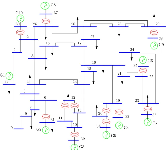
4.5 One line diagram of 39-bus New England power system . . . 79

4.6 Proposed versus Symbolic (direct Hessian) method for 39-Bus Power system. 80 4.7 Proposed vs Symbolic—Computation costs for 39-Bus Power System . . . 80

4.8 Distribution of G and H coefficients for the 145-Bus Power system . . . 81

4.9 Comparison of Linear, 2nd and 3rd order modal model for 39-bus system . . 82

4.10 Accuracy of the proposed method on detailed model with control . . . 89

4.11 Accuracy of the proposed method on 20- and 31-state system . . . 89

4.12 Distribution of C and D coefficients for 147-Bus Power System . . . 91

4.13 One-line Diagram of the IEEE 50-Machine 145-Bus Power system. . . 92

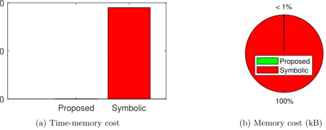
4.14 Time-Memory comparison of symbolic and proposed on 20-state system . . . 93

4.15 Two pathways for computing nonlinear coefficients . . . 94

5.1 Normal Form (NF) computation time for full and reduced models. . . 106

5.2 Modal decomposition of the G1 active power for less stressed condition (9-bus power system). . . 106

5.3 Modal decomposition of the G1 active power for stressed condition (9-bus power system). . . 108

5.4 Hankel singular values showing 5 most relevant states . . . 112

5.5 Participation factors of modes in the 5 hankel states . . . 112

5.6 Linear versus Nonlinear Participation Factors . . . 114

5.7 Frequency and damping ratio variations with generator power output. . . 118

5.8 Amplitude-dependent frequency shift during large disturbance. . . 119

5.9 F-A curve for the SMIB system . . . 121

5.10 Oscillations during large disturbance for 9-Bus Power System . . . 124

5.11 Oscillation during large disturbance for 145-Bus Power System . . . 126

5.12 Oscillation buildup for the WSCC breakup of August 10, 1996. . . 128

5.13 Rotor angle for different approximations and operating points (SMIB) . . . . 129

5.14 Marginally unstable system at 0.27 s clearing time for fault at bus 7 (145-bus power system). . . 134

5.15 Unstable system at 1.2 s clearing time for fault at bus 1 (145-bus power system)135

Introduction

“Things change. And friends leave. Life doesn’t stop for anybody.”

Stephen Chbosky

Contents

1.1 General Context and Motivation . . . 2

1.1.1 The Changing Grid . . . 2

1.1.2 Present and Potential Future Challenges of the Grid . . . 3

1.1.3 Need for Developing Tools in Continuity of the Existing Ones . . . . 6

1.1.4 Defining a Large Grid . . . 6

1.2 Tools for Power System Dynamic Performance Analysis . . . 7

1.2.1 Transient Stability Analysis . . . 7

1.2.2 Small-signal Stability Analysis . . . 8

1.3 Modes of Oscillation. . . 8

1.4 Modal Interactions and Nonlinear Modes . . . 11

1.5 Normal Form Method. . . 13

1.6 Objective and Scope of the Research. . . 14

1.7 Contributions of this PhD Research Work . . . 15

1.1

General Context and Motivation

1.1.1 The Changing Grid

Power system is an interconnection of many components such as generators, transformers, transmission lines and so on. The electric power is produced by the generators and trans-ported to the loads through the transmission lines. These lines can be short or long depending on the separation between the generation and loads. The electric power seems to be the most beneficial engineering innovation today. Therefore, to ensure a reliable and efficient power delivery, several intelligent techniques are being introduced into the power system. However, due to ratings and other constraints of the power system components, there is always a limit for operating the system, so called stability margins.

In the traditional power systems, the generators are mainly synchronous machines, mainly powered by environmentally-unfriendly sources like fossil fuel. Fossil fuel in turn is a key player in environmental degradation due to the accompanying emissions. The reduction of gas emissions and hence, fossil fuel, has been a worldwide concern owing to several negative environmental changes. With several economic, technical and environmental constraints, today’s power system is operated very close to its margins, making the system to be stressed. A stressed system has operating condition near, for example, the voltage stability limit and may be as a result of — 1) a higher level of system loadings, 2) heavy power transfer across some transmission interfaces, and 3) heavy loading of certain plants. This can be represented by a power-voltage (P-V) curve for bus voltage stability as shown in Figure 1.1. Stressed power system can lead to complex dynamic behaviour. That is, unusual nonlinear behaviour that could be difficult to explain.

V

V

Active Power

V

oltage

Loadability Margin

Normal condition

Stressed condition

The depletion of fossil fuel has forced a shift from traditional energy resources to renew-able energies (REs) such as solar thermal, solar photovoltaic, wind, and biogas [1]. Each year, more electricity is generated from renewable energy than in the previous year (see Fig-ure 1.2). The integration of these renewable energies into the grid is now feasible due to the technological advancements in power-electronic-based (PE) converters. The emergence of new PE devices onto the power scene and the increasing number of distributed genera-tion power systems in electrical grids contribute to changing the structure of the tradigenera-tional grid. This outburst seems to be the fastest growing trend in power system [2, 3] with pro-liferation of DC/AC inverters, switch mode power supplies, High Voltage DC (HVDC) links, distributed renewable energy systems, Static VAr Compensator (SVC), and other Flexible AC Transmission Systems (FACTS) devices.

Figure 1.2 – Annual Global Additions of Renewable Power Capacity, by Technology and Total, 2012-2018 [4]

1.1.2 Present and Potential Future Challenges of the Grid

The system stress together with the integration of RE increases the system nonlinearities and hence, creates new challenges to power systems. It can lead to nonlinear interactions of the system modes of oscillation, which alter the dynamic behaviour of the system. Mode is the technical term for a particular oscillation pattern (see detailed explanation in section1.3). The system nonlinearities and modal interactions are impacted by system operating conditions, control strategy, and control system parameters [5]. The transfer of large amount of power over long distances are not uncommon nowadays due to inter-area connections (example Scotland-England) and the growth of RE sources. Moreover, most viable RE sources like wind farms are usually far from load centre. The transfer of large power over long distances leads to power oscillations and nonlinear interactions in a High Voltage AC (HVAC) system.

HVDC links can be used instead, in order to damp the oscillations. However, the controls for HVDC can lead to strong nonlinear interactions, though these interactions are not always necessarily negative. Earlier investigation of nonlinear modal interaction in a HVDC/AC system with DC modulation indicated that strong nonlinear modal interaction can result from higher AC and DC loading and with well-tuned DC power modulation [5]. Perhaps, with the development of Modular Multilevel Converters (MMC) technologies, the situation may be different. Other PE devices also lead to increased nonlinearity. For example, the control parameter of SVCs can lead to strong nonlinear interactions in a stressed system, which gives rise to unstable oscillations [6]. Note that the controls of synchronous machines can equally introduce nonlinearities especially if not properly tuned [7]. However, [8] reported that nonlinear interaction is stronger when PE controls are in the system. With the growth of REs, utilising an additional device, such as battery energy storage (BES) in power systems is inevitable. A current research reported that increasing BES’s gain controller could lead to interaction events [9]. Since REs inject power into the network through PE converters, resulting in the lack of inertia and synchronising torque in the grid, de-commitment of the synchronous generators would increase the effect of nonlinearity [10] and will affect the rotor angle stability. Also, the PE converters could form a virtual capacitance, which could interact with the AC grid to trigger an unstable oscillation in relatively weak (i.e high impedance) system [11].

As highlighted in [12,13], apart from contributing to nonlinearity, REs and their accompa-nying PEs introduce new modes of oscillation to the grid due to displacement of synchronous machines. It was noted in [12] that these new modes of oscillation are highly sensitive to con-trol parameter variations, and can make the system more unpredictable and hard to monitor or control.

The challenges of RE/PE penetration to the grid have triggered serious researches in Eu-rope, mainly anchored by Massive Integration of Power Electronic Devices (MIGRATE) [14], which aims at finding solutions to the technical challenges. The MIGRATE’s report on sys-temic issues are summarised in Table 1.1. The manifestations of these challenges abound in practical power systems with significant RE integration. For example, on 19 February 2011, inter-area oscillations within the Continental Europe (CE) power system occurred. Similar oscillations reoccurred on 24 February, 2011. The oscillation frequency was 0.25 Hz and lasted for 15 minutes (see Figure 1.3). There was no clear clue on the cause of the oscillation ini-tially. Modal calculations in [16] later revealed that two modes superimposed at 0.25 Hz with participation of Turkey, Spain/Portugal and Italy against North of Europe. The following conclusions were made in [16]: (1) there was an interaction of 0.18 Hz (East-West mode) and

Table 1.1 – Ranking of the power system stability issues as identified by European TSOs in the context of the MIGRATE Project [15]

Ranking Ranking score Issue

1 17.35 Decrease of inertia

2 10.16 Resonances due to cables and PE 3 9.84 Reduction of transient stability margins

4 8.91 Missing or wrong participation of PE-connected generators and loads in frequency containment

5 8.19 PE Controller interaction with each other and passive AC components

6 7.50 Loss of devices in the context of fault-ride-through capability 7 7.00 Lack of reactive power

8 6.91 Introduction of new power oscillations and/or reduced damping of existing power oscillations

9 6.09 Excess of reactive power

10 4.27 Voltage Dip-Induced Frequency Dip

11 3.87 Altered static and dynamic voltage dependence of loads

0.25 Hz (North-south mode) modes, (2) synchronous connection of Turkey displaces 0.3Hz mode to 0.25 Hz (new mode), (3) the RE generators subtracted inertia from the system by replacing generators equipped withpower system stabilzer (PSS). Consequently, the Italian TSO immediately reinforced PSSs in Italy. Another severe oscillation occurred in Hami wind

Figure 1.3 – Detailed view of system frequency (measurements) for 19 February 2011— Brindisi (IT) in phase with Sincan (TR) and Recarei (PT) opposite to Portile de Fier (RO) and Kassoe (DK) [[16]

It was later found out that this oscillation was caused by the interaction between multiple wind turbine converters (WTCs) of permanent magnet synchronous generators (PMSGs) and the weak AC grid [17].

In the light of all these present and anticipated changes in the grid, it becomes necessary to extend the analysis of the grid in order to properly characterise its dynamic behaviour and to better design its controls. This will require more sophisticated tools to cope with the evolution. Although, there are several studies going on in respect to the increased nonlin-earity and consequent unusual behaviour of the grid, not much attention is being paid to the nonlinear interactions, which can reveal a lot of hidden information in the system. The effect of nonlinear interactions in a system can be negative or positive, depending on the condition of the system. This is perhaps, among other things, the reason why in literature, both positive and negative effects of RE/PE integration are being reported. For instance, improved damping of oscillations in case of an increasing share of PE-interfaced generation was reported in [18].

1.1.3 Need for Developing Tools in Continuity of the Existing Ones

As mentioned earlier, stressed systems exhibit strong nonlinear behaviour and the RE/PE integration into the grid further contributes to this stress. More sophisticated tools are needed to cope with the complexity of the system. Advanced tools such as Pattern Recognition methods [19], Expert Systems (ES) methods [20], Robust-control-based tools [21], are being developed for the study of complex systems. However, these tools are too far from the knowledge of an average power system operation engineer. Most often, they do not present quantifiable physical parameters to enable the engineer make decisions or plannings. The best known tool for studying oscillations in power system is modal analysis. The conventional modal analysis tools such as small-signal stability are commonly used. However, they are linear tools and will no more be sufficient to accurately characterise the behaviour of the grid when there is high penetration of RE/PE. There is therefore, a need to provide alternative tools with features common to the engineers and yet, with extended capabilities. Normal Form (NF) is a good alternative but it is difficult to apply to systems with large number of state variables.

1.1.4 Defining a Large Grid

Often times, when large grid/system is mentioned, what comes to mind is a power system with so many buses, lines, generators and so on. While this is logical, the meaning of large grid can be somewhat confusing. A grid could be large in the sense that there are many

interconnections and buses. A grid may also be considered large because of the computational difficulty in its analysis. The latter implies that, if power flow computation is considered, a 39-bus system for instance, is larger than a 9-bus system. This is because, the voltages at each bus and line flows have to be computed. On the other hand, if the dynamics of the state variables are to be considered, a 9-bus system with four machines, each modelled with 6 state variables may be considered larger that a 39-bus system with ten machines, each modelled with 2 state variables. Large system is used in this work in the sense of more state variables. The European interconnected system with about 20,000 state variables is commonly considered a large system. However, some new tools being developed for the future grid; such as the one considered in this work are extremely computation-intensive. As such, a system of 100 state variables for example may be considered large if a system with, say 20 variables, are sufficiently difficult to analyse. It is in this narrow context that large grid is used in this work.

1.2

Tools for Power System Dynamic Performance Analysis

The tools for the analysis of power system dynamic behaviour can be classified into two:

• nonlinear tools, which are suited for transient stability analysis.

• linear or small-signal analysis (SSA), which is based on the linear techniques and em-ployed for small-signal stability analysis.

1.2.1 Transient Stability Analysis

Transient stability is the capacity of the power system to remain in synchronism following a large disturbance. There are several methods for transient stability analysis, which are basically grouped into time domain simulations (TDS) and direct methods. TDS remains the most reliable method to investigate nonlinear systems. However, simulating a high di-mensional power grid could be very time consuming if oscillators are coupled and interact nonlinearly [22,23]. Moreover, it does not provide information regarding the degree of stabil-ity or instabilstabil-ity of a power system. It lacks in qualitative and structural information about the system.

Direct methods such as equal area criterion (EAC) and energy function techniques like boundary of stability region based controlling unstable equilibrium point method (BCU method) have their own strengths and weaknesses. EAC uses graphical visualisation to simplify sta-bility assessment, but limited to two-machine systems. Energy function methods are fast but not every post-fault transient stability model admits an energy function [24]. In addition

finding the controlling unstable equilibrium point (CUEP) by BCU is difficult. To enhance the transient stability analysis, it could be gainful to combine the TDS and the direct methods. This will reduce the challenges in each method.

1.2.2 Small-signal Stability Analysis

When a disturbance to the system is small enough, the system can be assumed to exhibit linear behaviour and can be analysed by linearising the system model around its steady-state operating points. The linearised model can provide many information not explicit in time-domain simulation. Stability determined with such model and with such assumption is called small-signal stability.

The first step involved is to linearise the power system differential equations in the neigh-bourhood of stable operating point. Then, the eigenvalues of the system are used to char-acterise the stability. The real part and the imaginary parts of an eigenvalue give damping and frequency information respectively. If the real part of the eigenvalue is negative, the amplitude of the oscillation decays and the system is stable. If the real part is positive, the amplitude increases and the system is not stable. For zero real part, the amplitude remains constant and more information is required for the stability. With the eigenvalues and eigen-vectors, it is possible to obtain an approximate close-form solution of the nonlinear differential equations with a given initial condition.

Small-signal stability analysis is a powerful tool for engineers. It presents the numerous mathematics describing the system in terms that are easy to understand and interpret. Just by observing the real part of an eigenvalue, an engineer has a feel of the likely behaviour of the system. SSAtool is almost indispensable in dynamic analysis. The challenge however, is that the analysis is limited to a neighbourhood of the operating point which the linearisation is valid.

1.3

Modes of Oscillation

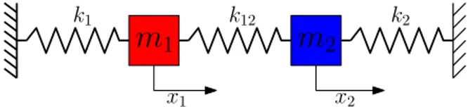
There are several modes of oscillations in an interconnected system. Mathematically, a mode (or an eigenmode)/natural mode is the term for one eigenvalue/eigenvector pair of the linear part of a dynamical system. Physically, a mode can be viewed as a unique pattern in which the stored energy in the system is expended when the system is disturbed. As an illustration, consider in Figure1.4, two masses m1, m2, attached to three springs k1, k2, and k12. Assume the end points are fixed, this system has two natural modes of oscillation.

m

1

m

k₁ k₁₂ k₂

x₁ x₂

Figure 1.4 – Mass-spring system exhibiting two natural modes of oscillation.

equations of motion of the system are given by

m¨x1 = −k1x1−0.3k1x21− 0.4k1x31+ k12(x2− x1) (1.1a)

m¨x2= −k2x2+0.4k1x22+ 0.3k1x32+ k12(x1− x2), (1.1b)

where nonlinearities (arbitrarily chosen) in the springs are intentionally added for demon-strations.

If we assume that the displacements are small enough and the equilibrium of the system is at the origin, the effects of the nonlinear terms (blue in (1.1)) can be neglected and it is possible to compute the natural frequencies in Hertz for identical springs and masses (i.e.,

k1 = k2= k12= k, m1 = m2= m) as f1 = 1 2π s k m, f2 = 1 2π s 3k m. (1.2)

Having assumed a linear system, when the mass m1 is moved by x1 to the right, the spring

k1 pulls the mass to the left with a reaction force k1x1, and the spring k12 pushes the mass to the left with a reaction force k12(x1− x2). Similarly, when the mass m2 is moved by x2 to the left, the spring k2 pulls the mass to the right with a reaction force k2x2, and the spring

k12 pushes the mass to the right with a reaction force k12(x2− x1). Assume k = 5, m = 1,

f1= 0.36 Hz and f2= 0.62 Hz. Thus, the two modes are described below :

• Mode 1 - both masses move together at frequency f1 = 0.36 Hz, with the same amplitude and in the same direction so that the connecting spring (k12) between them is neither stretched nor compressed. This motion is shown in Figure 1.5aand is obtained by simulating the nonlinear system (1.1) with small and equal initial conditions for

x1, x2. The FFT of Figure1.5b confirms the frequency of the oscillation.

• Mode 2 - both masses move at frequency f2 = 0.62 Hz, with the same amplitude but in opposite directions so that the connecting spring (k12) between them is alternately stretched and compressed. In this case, the center (node) of the connecting spring is stationary. This motion is shown in Figure 1.5c and is obtained by simulating the nonlinear system (1.1) with small, equal but opposite initial conditions for x1, x2. The FFT of Figure 1.5d confirms the frequency of the oscillation.

0 2 4 6 8 10 Time (s) -0.06 -0.04 -0.02 0 0.02 0.04 0.06 Displacement m1 m2 (a) Mode 1—0.36 Hz 0 0.5 1 1.5 2 Frequency (Hz) 0 2 4 6 8 Amplitude (b) Mode 1—FFT spectrum 0 2 4 6 8 10 Time (s) -0.05 0 0.05 Displacement m1 m2 (c) Mode 2—0.62 Hz. 0 0.5 1 1.5 2 Frequency (Hz) 2 3 4 5 6 7 8 Amplitude (d) Mode 2—FFT spectrum.

Figure 1.5 – Natural modes of Oscillation of two-mass three-spring system.

Any other motion of the bodies in Figure 1.4 is not natural but a linear combination of the two natural modes. The two modes described above have two distinct frequencies. Thus, mode is often used, more loosely, to refer to an oscillation at a characteristic frequency.

Power system can be modelled similar to the system in Figure 1.4, whereby the spring constant and the displacement are equivalent to the line impedance and rotor deviation respectively. The reaction force is analogous to the synchronising power of the power system. Let the force moving these masses represent the generator or fault power transported through the line. It can be seen from (1.1) and (1.2) that:

• Power flow on the lines can lead to oscillations.

• Higher impedance of the lines can lead to low frequency oscillation. • Higher impedance of the lines can weaken the ties between machines.

Using more elaborate models, major oscillations in power systems include: electrome-chanical, control, and torsional modes of oscillation. For electromechanical modes, the most involved variables are the internal angles and the rotor speeds of the generators. Generally speaking, power systems low-frequency oscillations are a result of electromechanical coupling between the transmission network and generators. Control modes are associated with gener-ator or the exciter units and other control equipment, such as poorly tuned exciters, HVDC converters, and static var compensators. Torsional oscillation modes are associated with the

turbine generator shaft rotational system. The major challenge of the power system is the low frequency electromechanical oscillations which can either be local or inter-area. When a machine or group of machines that have strong electric ties in an area oscillates and their oscillations are dominant in the area they are located, it is known as local oscillation. Inter-area mode involves machines in one Inter-area swinging against machines in other Inter-areas. It usually has lower natural frequency in the range of 0.1-0.8Hz [25]. However, with several converter control-based generators (CCBG) devices in the grid, the above characteristics may not al-ways be true signatures of electromechanical modes. This is because the CCBGs lead to new low oscillatory modes akin to the inter-area electromechanical modes of oscillation [12]. This phenomenon poses a problem in identifying clearly, the actual electromechanical modes. New methods are being developed to tackle this problem [26]. Analysis of large systems has to necessarily focus on the critical modes of importance, usually the inter-area modes.

The study of the behaviour of these modes is known as modal analysis. The most common tool for modal analysis is the SSA which provides much information regarding these oscil-lations. Since SSA explains only linear behaviour, it is more precisely referred to as Linear Modal Analysis (LMA).

1.4

Modal Interactions and Nonlinear Modes

When the power system is stressed, the dynamics are not completely described by the natural modes. In addition to the natural modes, the dynamics can be affected by some higher order combinations of the natural modes. The effect of these higher order combinations is called nonlinear modal interaction. The nonlinear modal interaction gives rise to ”other modes”, which may significantly affect the dynamics of the system. The mechanism, by which these ”other modes” are formed, will be clearly explained, mathematically, in later chapters. The concept of nonlinear mode allows for proper understanding, and interpretation of the phenomenon—nonlinear modal interaction, since it helps to explain the ”other modes”, with the eigenspectrum. Nonlinear mode is used to describe the extension of a linear mode to the nonlinear regime. Thus, it is an extension of theinvariance property of a linear mode to the nonlinear regime. Physically, it is the rendering of nonlinear modal couplings, in a way that, if a particular motion is initiated on a particular mode only; no energy is given to the others, such that the motion remains on this mode only.

Modal interaction is critical and can either stabilise or destabilise the system. For instance, the excitation system can introduce modes which interact with the electromechanical modes of the system, resulting in angle instability. When nonlinear modal interaction occurs, the

dynamics become difficult to explain withLMA. The modal analysis which takes into account the nonlinear interactions of modes is known asNonlinear Modal Analysis (NLMA).

A simple illustration of nonlinear modal interactions can be shown by simulating the system (1.1) with higher initial conditions (i.e larger displacements of x1, x2). The effect of the nonlinearities will no longer be negligible and the oscillation will be composed of the linear (natural) and significant combinations of the linear modes. This is shown in Figure 1.6. It is clear from Figure 1.6a that mode 1 is dominant. At least, the response resembles the one in Figure 1.5a. However, the conclusion that linear mode is sufficient

0 2 4 6 8 10

Time (s)

(b) FFT showing—linear and nonlinear modes.

Figure 1.6 – Example of modal interactions

to understand the behaviour of that system can be deceptive. The FFT in Figure 1.6b

clearly reveals the significant presence of other frequencies, in this case, due to nonlinear distortions of the natural modes. For example, the two linear modes are identified (0.36 Hz and 0.62 Hz) with mode 2 having smaller peak. Observe that there is a frequency of 0.72Hz (i.e., 0.36 + 0.36 = 2 × mode 1), whose amplitude is high. There is also a frequency of 1.08 Hz (i.e., 0.36 + 0.36 + 0.36 = 3 × mode 1), although with smaller peak. In a way, one can loosely say, there are ”new modes” in the dynamics other than the linear modes. A common term usually used to describe these new frequencies is nonlinear harmonics, since they are multiples of the fundamental modes. However, as we shall see in later chapters, these new frequencies are not necessarily multiples of a fundamental mode but can come from combinations of different modes. NF provides analytical way to clearly explain the sources of these frequencies. When a power system is stressed, this phenomenon is present. Therefore, other information is needed in addition to linear analysis to properly understand the behaviour.

There are basically two approaches for detecting nonlinear modal interactions in a system— time-domain-simulation-based methods and closed-form solution methods. In case of time domain simulation, the time responses are extracted, and then, their spectral components

decomposed with some tools like Hilbert spectra analysis (HSA), Prony analysis or FFT (though other methods have been proven to be more efficient). By evaluating the damping and the frequency, the mode combination leading to a new mode with significant amplitude can be predicted. The comparison of the new mode with the natural modes can show possi-ble interaction. The second method extends theLMA to obtain closed-form solution of the nonlinear approximate model of the system. Then, it enables some definitions which exactly detect the interacting modes and the new frequency. The most common tool in the second category is theNFtool. NFmethod has advantage in that it does not only detect the nonlin-ear interaction, but also, it renders the system in such a way that the convenient techniques in LMA can still be employed to describe the system. In other words, it provides a good way to explain the concept of nonlinear modes. However, it has very serious computational challenges. The two approaches can be used in a complementary way. Thus, time domain simulation can be used to verify the solutions fromNF method.

1.5

Normal Form Method

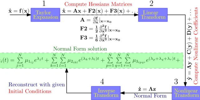
The term Normal Form is used in several domains for various connotations. For example, it is used to refer to database normalisation. In mathematics and computer science, it can mean any standard way of presenting object as a mathematical expression. Example in this case is the Jordan normal form. Normal Form as used in this work is a mathematical technique that simplifies a set of nonlinear differential equations into a simplified one, which can be linear in some particular cases. The simplification is achieved by introducing sequential nonlinear coordinate transformations. The resulting equations are then in their simplest form (Normal Form) [27–30]. This definition of Normal Form is often precisely referred to, as Poincar´e Normal Form, after the work of Poincar´e [27]. It is based on the series expansion of a system of nonlinear differential equations. The NF technique itself is very old but its power system application to nonlinear modal analysis is quite on the trend. In the last two decades, researchers at Iowa state university made several publications and promoted the need to study higher order modal analysis with Normal Form. Their propositions received concern and in 2005, an IEEE task-force was formed to investigate on the need for inclusion of the higher order terms in small-signal analysis. The task-force highlighted the potentials of NF

technique and recommended its higher order development in future [31].

The NF approach consists of obtaining a higher order Taylor series expansion of the nonlinear equations around a stable equilibrium point (SEP). The linear part of the series expansion is analysed to extract the modal contents. With the modal parameters of the linear

part, it is possible to define some coordinate change of variables which simplify the nonlinear parts.

The higher order NFaccounts for sufficient nonlinearities and hence, will be suitable for studying the developments in today’s grid, and even in future. This has been demonstrated on grid with high penetration of RE/PE in [10].

1.6

Objective and Scope of the Research

The implication of all the changes going on in today’s grid is that the LMA tools designed for its analysis begin to fail. Yet, the features of LMA tools are so attractive that losing them will be difficult. Among the nonlinear alternatives, NF method has received highest research interest up till present day. NF tool has however, a major setback that limits its application in power system. It is computationally very expensive. Traditional approach requires the preliminary evaluation of Hessian matrices and eigenvalue expansion, which are impracticable with standard methods when considering large scale systems. The process of the eigenvalue expansion is very difficult and needs to be accelerated. In order to improve on this global power system problem and make nonlinear modal analysis of the future grid possible, this thesis principally deals with one issue:

• The drastic reduction of the computations needed to apply NF method to power systems with large number of state variables (so-called large systems).

The thrust of the work is therefore, the simplification of processes forNFapplication in power systems. A new method for rapidly evaluating all polynomial coefficients (termed nonlinear coefficients in this work) needed for NF application is proposed. It is assumed that the computation of all eigenvalues is possible and the power system network is already reduced if necessary. Proposed method was applied to four different systems: the IEEE 3-, the IEEE 10-, the IEEE 16-, and the IEEE 50-machine systems. Known applications of NF, such as participation factor analysis, stability and nonlinear frequency shift predictions are reviewed and implemented with drastically reduced computation. The other scopes of the research work are as follow:

• It is assumed that the nonlinearities are smooth and static. By smooth nonlinearities, it means that the system nonlinearities considered are that which can be represented by the higher order terms in the Taylor series expansion for the set of system differential equations. By static nonlinearities, it means that the nonlinearities are not on the differential parts (terms) of the system model but on the algebraic parts (terms). The second and third order terms of the equations of the power system are considered in

this research work. However, higher orders can be considered if deemed necessary and practicable.

• The LMA is performed to extract the fundamental mode of oscillations of power sys-tem and associated eigenvectors. Then with the eigenvectors, the original syssys-tem is transformed to Jordan form.

• The same Jordan transformation is extended to the nonlinear parts of the Taylor ex-pansion. But the Jordan transform equivalent for the second and third order terms are estimated with the modal parameters obtained from the LMA. The original system is perturbed using the eigenvectors to evaluate the components of the Jordan transform of the higher order terms (i.e. nonlinear coefficients).

• Both real-valued and complex-valuedNFare considered for second order and first order power system models respectively. For the second order model, the theory ofnonlinear normal mode (NNM)adapted from mechanical engineering domain is extended to study power system oscillation.

• New method for selective application ofNFto the study of nonlinear modal interactions was proposed. Previous indices for nonlinear modal interactions were used to study modal interactions based on the selective method for NFproposed.

• Based on NNMtheory, a new method for monitoring instability of modes in a multi-machine power system was developed.

• The time simulations were conducted to verify inferences made from NF technique, regarding the system dynamic behaviour.

Therefore, the research work utilises a combination of normal form theory, nonlinear normal mode theory, linear system techniques, Taylor series expansion, mode excitation technique, and time-domain simulation.

1.7

Contributions of this PhD Research Work

In response to the research problem, this thesis has made the following contributions:

1. To the knowledge of the author, this thesis is the first application ofNFto power system study without the usual preliminary Taylor series expansion. This thesis proposes a fast method to obtain the needed nonlinear coefficient for NF model without Taylor expansion and the associated Hessian matrices computation. By avoiding the building of Hessians, the NFanalysis becomes fast.

2. In terms of NF application to second order power system model, this thesis reports the largest test case ever, considering third order nonlinearities. The application ofNF

to second order power system model without any complex variables, using NNM is a new concept not well exploited. To the author’s knowledge, the largest reported test case of such application involves only four generators. The technique developed in this thesis allows the extension of the capability of the previous proposals to the study of more than fifty machines in a convenient computational time.

3. This thesis introduces new and computationally-reduced tool for monitoring electrome-chanical mode instability in an interconnected power system. The proposed method has potential for on-line application and can be used by power system operators to make quick and rough estimation of modes’ proximity to instability.

4. The new approach to NF analysis proposed in this thesis opens the way for selective

NFapplication in power systems. For example, this thesis proposes a fastNFtechnique for power system modal interaction investigation, which uses characteristics of system modes to carefully select relevant terms to be considered in the analysis. This leads to a very rapid nonlinear modal analysis.

5. To the author’s knowledge, there is no dedicated software for NF application due to its computational complexities. The proposed method allows the reuse of only the information from linear analysis, to evaluate the coefficients of all nonlinear terms, in a linearly-simple and computer-friendly fashion. Thus, the implementation ofNF with power system commercial software like EUROSTAG®, which already has linear and transient analysis tools embedded, is achievable.

6. Although certain constraints precluded some further experimentation and validation, this thesis opens up several research problems for future researchers. For instance, the criteria proposed for selective NF applications can be investigated for 100% PE grid. Also, further computational reduction using balanced realisation technique was suggested. This could be well explored for very large systems.

Some of the main contributions of this thesis are validated by the following articles which were drawn from it:

• N. S. Ugwuanyi, X. Kestelyn, O. Thomas, B. Marinescu and A.R. Messina, “A New Fast Track to Nonlinear Modal Analysis of Power System Using Normal Form,” IEEE Trans. Power Syst., vol. 35, no. 4, pp. 3247-3257, 2020.

• N. S. Ugwuanyi, X. Kestelyn, B. Marinescu and O. Thomas,“Power System Nonlinear Modal Analysis using Computationally Reduced Normal Form Method,”Energies, vol. 13, no. 5, p. 1249, 2020.

• N. S. Ugwuanyi, X. Kestelyn, O. Thomas, and B. Marinescu, “A Novel Method for Accelerating the Analysis of Nonlinear Behaviour of Power Grids using Normal Form Technique,” in Innovative Smart Grid Technologies Europe (ISGT Europe), 2019.

• N. S. Ugwuanyi, X. Kestelyn, O. Thomas, and B. Marinescu, “Selective Nonlinear Coefficients Computation for Modal Analysis of The Emerging Grid,” in Conf´erence des Jeunes chercheurs en G´enie El´ectrique, 2019.

• N. S. Ugwuanyi, X. Kestelyn, B. Marinescu, and O. Thomas, “Speedy Technique for Selective Nonlinear Analysis of Electromechanical Modes of Future Grids,” European Journal of Electrical Engineering: UNDER REVIEW.

1.8

Thesis Outline

The thesis is divided into 6 chapters described as follows.

Chapter 1 provides context as well as the statement of the problem. The motivation, objectives and the main contributions of this research work are also presented in this chapter.

Chapter 2 presents a detailed literature review dedicated to Normal Form applications in power systems, challenges, and the existing proposals to mitigate these challenges. Some background information are presented as well. Also, the scientific position of the current work globally and in L2EP1 is established in this chapter.

Chapter 3 describes the power system models used in this work and the Normal Form method due to these models. Simple examples are used to explain the NFmethod. Also, in this chapter, the challenges encountered inNFapplications are discussed and demonstrated.

Chapter 4 presents a detailed documentation of the proposed method for computing all the nonlinear coefficients, both for second and first order power system models. Examples are presented to explain the method. Thereafter, several larger systems are tested. The pro-posed method is compared with symbolic tool and the computational efficiency and accuracy

1

L2EP is the french research laboratory in which the present PhD was prepared. L2EP stands for Labo-ratory of Electrical Engineering and Power Electronics

extensively discussed in this chapter. Also, the time domain simulations are presented to support the results.

Chapter 5 presents the practical power system applications of NF method facilitated by the proposed method. In this chapter, new proposals for studying power systems based on

NNM are presented and validated with numerical simulations on IEEE 3- and IEEE 50-machine power systems. Also in this chapter, new approaches for selective study of modal interactions and participation factors are presented.

Chapter 6 presents conclusions of this work and suggestions for future work.

Finally, the details of the third order normal form for the power system equations and the data for the IEEE 3-machine system are given in Appendices D and E respectively. Other interesting appendices are also presented.

Literature Review

“That is part of the beauty of all literature. You discover that your longings are universal longings, that you’re not lonely and isolated from anyone. You belong.”

F. Scott Fitzgerald

Contents

2.1 Revisiting Linear Modal Analysis Tools . . . 20

2.2 Basic Idea of Normal Form . . . 26

2.3 Applications of Normal Form in Power Systems . . . 27

2.3.1 Higher Order Normal Form Methods Existing in Literature . . . 29

2.3.2 Real Normal Form Transformation . . . 31

2.3.3 Summary of NF Applications in Power Systems. . . 32

2.4 Present Challenges with Normal Form Method . . . 32

2.5 Power System Model Order Reductions . . . 36

Introduction

In chapter 1, it was stated that the thrust of the thesis is the simplification of the process involved in Normal Form application. It was also stated that stressed systems exhibit increased nonlinearities which lead to nonlinear modal interactions. These interactions can be positive or negative, phenomena beyond the scope of linear analysis. The exploration on the NF method, advocated since last two decades by researchers in IOWA state university; and later by other laboratories in USA, Mexico, Japan, China, and recently France (L2EP1), highlights NF’s potentials for better analysis of stressed systems ( hence, for present and future grids). Several other research laboratories worldwide are working on Normal Form method and its applications to modal analysis, both in power systems and in other fields. This chapter is dedicated to the review of NF applications in power systems. The aim of the reviews is to bring out the relevance of Normal Form as a tool in power systems; its challenges and the existing proposals to mitigate these challenges. The position of the thesis globally is then established. The reviews are sectioned for easy reading and some background information are provided. The chapter starts with a concise appraisal of linear modal analysis, upon which the developments of nonlinear modal analysis are based. The idea is to show the rich features of linear analysis which are emulated and expanded by the Normal Form.

2.1

Revisiting Linear Modal Analysis Tools

Linear modal analysis is widely applied in power systems to study and provide solutions to oscillation problems. The dynamical behaviour of power systems can be represented by

˙

x = f (x, u), (2.1a)

0 = g(x, u). (2.1b)

In (2.1), x is a vector of the state variables and u is a vector of input. The expressions of x depend on the model being considered. A system described with differential equation (2.1a) and the algebraic equation (2.1b) is said to be adifferential-algebraic-equations (DAEs)

system. A linear model is obtained by linearising the nonlinear system around an operating point, usually performed in the neighbourhood of SEP.

Assume x0, u0 to be initial state vector and the input vector respectively, which

corre-spond to the equilibrium point, then, x(x0, u0) is the solution of (2.1) with ˙x = 0. For small

perturbation, the new states and inputs are denoted as x = x0+ ∆x, u = u0+ ∆u, where

1

L2EP is the french research laboratory in which the present PhD was prepared. L2EP stands for Labo-ratory of Electrical Engineering and Power Electronics

∆ stands for increment. Linearisation is an assumption that if the perturbation is sufficiently small, first term of the Taylor series expansion can approximate the dynamics of the nonlinear system. It is possible to put the algebraic equations into the differential ones. Therefore, the linear model is given by

∆ ˙x = A∆x + B∆u, (2.2a)

(2.2b)

where the Jacobians, evaluated at theSEPare:

A = ∂f

∂x|x0,u0, B =

∂f ∂u|x0,u0.

Under free motion (i.e. zero input), the system (2.2a) can be be written as

∆ ˙x = A∆x. (2.3)

The equilibrium can be shifted to the origin so that the vector of state variables x represents perturbations from the equilibrium. Therefore, the linear model under free oscillation is given as

˙

x = Ax. (2.4)

The eigenvalues and eigenvectors are computed from A by solving the following eigenvalue problem (A − λI)U = 0, where I is an identity matrix, U is a matrix with each column corresponding to one eigenvalue λi of the system, so called right eigenvectors. With the right

eigenvectors determined, the complementary vector V is determined by solving VA = λV, where V is a matrix with each row corresponding to an eigenvalue, so called left eigenvectors. Participation factor is defined with left and right eigenvectors as

Pki= vkiuki. (2.5)

where vki and ukidenote the k-th components of the eigenvectors viand ui. The participation

factor is a dimensionless quantity which represents the measure of the participation of the state variable xk in the i-th mode.

In LMA, it is not always easy to isolate the parameters that significantly affect the dy-namics due to the cross-couplings existing among the state variables. These cross-couplings are removed by putting the linear model in Jordan form. Jordan form is obtained by in-troducing a new state variable through a linear transformation, using the eigenvectors. The

linear transformation (also called similarity or near identity transformation) is of the form

x = Uy, (2.6)

where y is the vector of the new state variable.

Differentiating (2.6) and substituting into (2.4) yields

U ˙y = AUy. (2.7)

Pre-multiplying both sides of (2.7) by the left eigenvector matrix yields

˙

y = Λy, (2.8)

where Λ = VAU is a diagonal matrix with the eigenvalues on the diagonal. The system (2.8) is said to be in Jordan form since the eigenvalues are distinct. Since the system is now decoupled, each element of y corresponds to a particular eigenvalue (mode). Thus, the variable y is also called modal variable and the model (2.8), modal model.

Hence, the solution of (2.8) for the i-th Jordan form variable can be written as

yj(t) = yj0eλjt, (2.9)

where yj0is the j-th initial condition in the Jordan form coordinate system. Then the

closed-form linear solution in the original machine states for an N -differential system is obtained by using the transformation in (2.6) as

xi(t) = N

X

j=1

uijyj0eλjt ∀i, j = 1, 2, . . . , N, (2.10)

where uij is the element in the i-th row and j-th column of the right eigenvector U.

Countless number of researches and publications exist, based on linear analysis. It has been used to analyse power system’s inter-area oscillation phenomenon in [25,32–34]. Sen-sitivity analysis performed in linear analysis helps to understand which state variable (and from which machine) participates more in a particular mode. It also helps to know which groups of machines will swing together or against themselves when a mode is excited. With the linear techniques such as observability and controllability, the system eigenvectors can help in designing power system controls [35]. Also, it helps to know the optimum location for siting PSS [36]. Linear tools have gained even much wider usage with the developments in power electronic converters. Researchers in L2EP are developing several control strategies

forpower electronic (PE)converters for power grid, based on the linear analysis [37–39]. To illustrate the benefits of LMA, let us consider the system in Figure2.1. The complete data for the system are presented in Appendix E. Each of the machines is represented with 2 state variables (rotor angle and speed), which means the size of the system is 6.

G1

G2

G3

2

7

8

9

3

6

5

4

1

Area 2

Area 1

Figure 2.1 – IEEE 3-machine 9-bus power system

The eigenvalues of the system are given in Table 2.1. Without time-domain simulation, Table2.1 shows immediately, at least, three important features of the system—(1) there are two modes of oscillation with frequencies 2.2 Hz (local) and 1.4 Hz (inter-area)2; (2) these modes are stable since they have negative real parts; and (3) these modes are poorly damped since they have real parts near to zero and damping ratios much less than 5%. The work of a control designer, is to ”push” the real parts of these modes (eigenvalues) far into the negative half-plane.

Table 2.1 – Eigenvalues

Mode Eigenvalue Frequency (Hz) Damping ratio (%)

λ1,2 -0.0147±13.72j 2.20 0.11

λ3,4 -0.0075 ± 8.82j 1.40 0.09

λ5 -0.0087 0 100

λ6 -0.00 0

-Table2.2shows the participation factor analysis corresponding to the system modes. The participation factors give another vital information not apparent in time-domain simulations.

2

Recalled from chapter 1, Inter-area oscillation mode involves machines from different areas, while local oscillation mode involves machines in a particular area.

It is clear that mode 1 is more associated with G2 and G3, while mode 2 is more associated to G1 and G2. To improve the damping of mode 1 for instance, it is better to locate thePSS

in the area of the system closer to G3. The location of the PSSin the area closer to G1 may be a bad choice. In the same vein, location of the PSS in area of G2 is more preferable for improving the damping of mode 2.

Table 2.2 – Mode-in-state participation factors (absolute values) for the system modes

λ1 λ2 λ3 λ4 λ5 λ6 State 0.0032 0.0032 0.1284 0.1284 0.3564 0.3804 δ1 0.0032 0.0032 0.1284 0.1284 0.0000 0.7368 ω1 0.1033 0.1033 0.3081 0.3081 0.3163 0.1393 δ2 0.1033 0.1033 0.3081 0.3081 0.0000 0.1770 ω2 0.3934 0.3934 0.0635 0.0635 0.3273 0.2411 δ3 0.3934 0.3934 0.0635 0.0635 0.0000 0.0862 ω3 | {z } | {z } Mode 1 Mode 2

Furthermore, by plotting the right eigenvectors corresponding to the angles of the ma-chines, it is possible to determine how the machines in the system will swing, should any of the modes be excited. Such plots are known as the mode shapes and are shown in Figure2.2.

90 270 180 0 G1 G2 G3 (a) Mode 1 90 270 180 0 G1 G2 G3 (b) Mode 2

Figure 2.2 – Mode shapes for the two oscillatory modes

Figure2.2ashows that if mode 1 is excited, G2 and G3 will swing in 180◦phase opposition. G1 is not apparent in the figure because its participation to this mode is very low. If the system in Figure 2.1 is considered a two-area power system, then mode 1 can be viewed as local modes, since G2 and G3 are in one area. Figure 2.2b shows that when mode 2 is excited, G2 and G3 will swing together and in 180◦ phase opposition with G1. This mode can be viewed as inter-area, since G1 is in one area while G2 and G3 are in another area. The information provided by mode shapes can be used as a guide in aggregating machines or

model order reductions [see,40].

To observe these oscillations in time-domain simulation, let us try to excite these modes almost separately. Since mode 1 is more associated to G3, it can be excited by a disturbance near G3. A three-phase fault at bus 9, applied at 1 s and cleared after 0.01 s produces the response in Figure2.3a. It is clear that G2 and G3 are in phase opposition at approximately

0 1 2 3 4 5 6 7 8 9 10 Time (s) 0.9985 0.999 0.9995 1 1.0005 1.001 (p.u) G1 G2 G3 (a) Mode 1 0 1 2 3 4 5 6 7 8 9 10 Time (s) 0.997 0.998 0.999 1 1.001 (p.u.) G1 G2 G3 (b) Mode 2

Figure 2.3 – Excitation of the two oscillatory modes

2.2 Hz, with G1 almost unaffected. This is in agreement with theLMA in Figure 2.2a. A disturbance at bus 2 will excite mode 2, but also significantly excite mode 1. This is because G2 has also significant participation in mode 1. In general, inter-area modes involve many machines in the system and can be difficult to excite without significant excitation of some local modes. Since G1 has very low participation in mode 1, a disturbance near G1 will excite mode 2 with minimum excitation of mode 1. A three-phase fault at bus 4, applied at 1 s and cleared after 0.01 s produces the response in Figure2.3b. The observed oscillation is coherent with theLMA result of Figure 2.2b.

Notice that in Figure2.3, it is easy to observe the pattern of the oscillations, but it is not easy to pinpoint the exact states responsible. Indeed, linear analysis provide very interesting characteristics of a system which are not very apparent in time-domain simulation tools.

As seen in chapter 1, the response of the power system is considered most often as a combination of natural modes of oscillations present in the system. The eigenvalues obtained from linear analysis should represent the fundamental frequencies which are observed in the motions of the different machines in the system. It was also shown in chapter 1 that in a stressed system with significant nonlinearity, the linear analysis may not be able to charac-terise properly the dynamics due to significant modal interactions and harmonic distortions. However, as seen above, it will be difficult to totally get rid of LMA due to the information it provides. Moreover, the nonlinear effects can be better understood as the combinations of these linear modes. As [41] says, ”The nonlinear effects should be considered as additions