HAL Id: tel-00597513
https://pastel.archives-ouvertes.fr/tel-00597513
Submitted on 1 Jun 2011HAL is a multi-disciplinary open access archive for the deposit and dissemination of sci-entific research documents, whether they are pub-lished or not. The documents may come from teaching and research institutions in France or abroad, or from public or private research centers.
L’archive ouverte pluridisciplinaire HAL, est destinée au dépôt et à la diffusion de documents scientifiques de niveau recherche, publiés ou non, émanant des établissements d’enseignement et de recherche français ou étrangers, des laboratoires publics ou privés.
Applications of digital topology for real-time markerless
motion capture
Benjamin Raynal
To cite this version:
Benjamin Raynal. Applications of digital topology for real-time markerless motion capture. Other [cs.OH]. Université Paris-Est, 2010. English. �NNT : 2010PEST1038�. �tel-00597513�
ECOLE DOCTORALE MSTIC
Th`ese pour obtenir le titre de docteur de l’Universit´e Paris-Est Sp´ecialit´e : Informatique
Soutenue et pr´
esent´
ee publiquement par
Benjamin RAYNAL
Sous la direction de Michel COUPRIE
Applications de la Topologie Discr`
ete pour
la Captation de Mouvement en Temps R´
eel
et Sans Marqueurs
7 December 2010
Composition du jury :
Rapporteurs : Edmond BOYER
Luc BRUN
Examinateurs : K´alm´an PAL ´AGYI
Hideo SAITO Michel COUPRIE Vincent NOZICK
Title:
Applications of Digital Topology For Real-Time Markerless Motion Capture
Abstract
This manuscript deals with the problem of markerless motion capture. An approach to this problem is model-based and is divided into two steps: an initialization step in which the initial pose is estimated, and a tracking which computes the current pose of the subject using infor-mation of previous ones. Classically, the initialization step is done manually, forbidding the possibility to be used online, or requires constraining actions of the subject.
We propose an automatic real-time markerless initialization step, that relies on topological information provided by skeletonization of a 3D reconstruction of the subject. This topological information is then represented as a tree, which is matched with another tree used as model description, in order to identify the different parts of the subject. In order to provide such a method, we propose some contributions in both digital topology and graph theory research fields.
As our method requires real-time computation, we first focus on the speed optimization of skeletonization methods, and on the design of new fast skeletonization schemes providing good results.
In order to efficiently match the tree representing the topological information with the tree describing the model, we propose new matching definitions and associated algorithms.
Finally, we study how to improve the robustness of our method by the use of innovative con-straints in the model.
This manuscript ends by a study of the application of our method on several data sets, demon-strating its interesting properties: fast computation, robustness, and adaptability to any kind of subjects.
Keywords
markerless; motion capture; digital topology; thinning; alignment; homeomorphism; betweenness.
Applications de la topologie discr`ete pour
la captation de mouvement en temps r´eel et sans marqueurs.
R´
esum´
e
Durant cette th`ese, nous nous sommes int´eress´es `a la probl´ematique de la captation de
mouve-ment sans marqueurs. Une approche classique est bas´ee sur l’utilisation d’un mod`ele pr´ed´efini
du sujet, et est divis´ee en deux phases: celle d’initialisation, o`u la pose initiale du sujet est
estim´ee, et celle de suivi, o`u la pose actuelle du sujet est estim´ee `a partir des pr´ec´edentes. Sou-vent, la phase d’initialisation est faite manuellement, rendant impossible l’utilisation en direct, ou n´ecessite des actions sp´ecifiques du sujet.
Nous proposons une phase d’initialisation automatique et temps-r´eel, utilisant l’information topologique extraite par squelettisation d’une reconstruction 3D du sujet. Cette information est repr´esent´ee sous forme d’arbre (arbre de donn´ees), qui est mis en correspondance avec un arbre utilis´e comme mod`ele, afin d’identifier les diff´erentes parties du sujet. Pour obtenir une telle m´ethode, nous apportons des contributions dans les domaines de la topologie discr`ete et de la th´eorie des graphes.
Comme notre m´ethode requiert le temps r´eel, nous nous int´eressons d’abord `a l’optimisation du temps de calcul des m´ethodes de squelettisation, ainsi qu’`a l’´elaboration de nouveaux algorithmes rapides fournissant de bons r´esultats.
Nous nous int´eressons ensuite `a la d´efinition d’une mise en correspondance efficace entre l’arbre
de donn´ees et celui d´ecrivant le mod`ele.
Enfin, nous am´eliorons la robustesse de notre m´ethode en ajoutant des contraintes novatrices au mod`ele.
Nous terminons par l’application de notre m´ethode sur diff´erents jeux de donn´ees, d´emontrant ses propri´et´es: rapidit´e, robustesse et adaptabilit´e `a diff´erents types de sujet.
Mots Cl´es
captation de mouvement sans marqueurs; topologie discr`ete; squelettisation;
Acknowledgements
First and foremost, I wish to thank my supervisors: Michel Couprie for his numerous and precious advices, his patience and all the other things which are too long to enumerate; Vincent Nozick, especially for his infectious enthusiasm, his support and his friendship, and many other things.
Over the three past years I have enjoyed working in the A3SI team, in a good mood and with very competent researchers. I wish to thank Venceslas, Gilles, Jean, Denis, Yukiko, Hugues, Laurent and Dror for their good advices and their attention. I specially thank my fellow PhD students, Franois-senpai, Patrice-senpai, Yohann, John, Fabrice, Anthony, Adrien, Camille, Olena (special thanks for you, for all the time you spent to read my thesis ;) ) and Nadine for all the time spend together, for their support and their friendship.
From my point of view, the LIGM is a great lab, thanks to its awesome members, who taught me almost all I know concerning computer science, from the basics to my actual level. I wish to specially thanks Marc, Nicolas, Marie-Pierre, Eric, Etienne, Cyril, and Jean-Christophe for this reason, and Julien, Elsa and Nelly for their friendship.
In a more general way, I would like to thanks my Dad who transmits me his passion for the computers, my Mom who always encourages me to do what I wanted, my big brother who shows me the way of the research and my little sister, well, you know... for being my little sister. Special thanks to Florian and Damien, who believe in me and are my friends since more than twenty years.
Finally, I would like to thank my fianc´ee Celine, for her patience, her kind, her tenderness, and her love.
Contents
Abstract iv
Acknowledgements vi
List of Figures xiii
List of Tables xvii
I Introduction 1
1 Global Introduction 3
1.1 Background . . . 3
1.2 Contribution . . . 4
2 Motion Capture Overview 5 2.1 Overview of Motion Captures Systems . . . 6
2.1.1 Acquisition Systems Using Markers. . . 6
2.1.2 Marker Free Optical Acquisition Systems . . . 6
2.2 A priori Model Definitions . . . 8
2.2.1 Adaptability of the Models . . . 9
2.3 On the Use of Multi Camera Systems . . . 10
2.3.1 Projection in Images . . . 10
2.3.2 3D Reconstruction of the Subject . . . 10
2.3.2.1 Stereo-Correlation . . . 10
2.3.2.2 Visual Hulls . . . 11
2.4 Initialization Step of Model-Based Methods . . . 12
3 Motivation 13 3.1 Model Definition . . . 13
3.1.1 Constraints of Descriptors . . . 13
3.1.2 Model Description . . . 14
3.2 Initialization Method Overview . . . 15
3.2.1 Extraction of Data Tree . . . 15
3.2.2 Matching Data Tree with Model Tree . . . 16
3.2.3 Pipeline and Main Difficulties of Our Method . . . 17
II Skeletonization Optimizations 19
4 State of the Art of Skeletonization 21
4.1 Thinning Theory . . . 22
4.1.1 Definitions and Notations . . . 22
4.1.1.1 Neighborhood . . . 22 4.1.1.2 Connectivity . . . 23 4.1.1.3 Connectivity Numbers. . . 24 4.1.2 Simple points . . . 25 4.1.2.1 Simple Points in 2D . . . 25 4.1.2.2 Simple Points in 3D . . . 25
4.1.2.3 Simple Points in Higher Dimensions . . . 26
4.2 Different Kind of Skeletons . . . 26
4.2.1 Ultimate Skeleton . . . 26
4.2.2 Curvilinear and Surface Skeletons . . . 27
4.2.2.1 Extremity Points. . . 28
4.2.2.2 Isthmus . . . 28
4.2.2.3 Symmetric versus Asymmetric Skeletons . . . 29
4.3 Thinning Algorithms . . . 29
4.3.1 Sequential algorithms . . . 29
4.3.2 Parallel algorithms . . . 31
4.3.2.1 Directional Algorithms . . . 32
4.3.2.2 Subfield-Based Algorithms . . . 33
4.3.2.3 Fully Parallel Algorithms . . . 34
5 Faster Implementation of Thinning Schemes 37 5.1 Classical Optimizations . . . 37
5.1.1 Restriction of Points to Check . . . 37
5.1.2 Optimization of Deletion Conditions Tests. . . 38
5.1.2.1 Usage of Look-Up Tables . . . 38
5.1.2.2 Usage of Binary Decision Diagrams . . . 39
5.1.2.3 Look Up Tables versus Binary Decision Diagrams . . . 41
5.2 Look Up Tables for Critical Kernel Based Algorithms . . . 41
5.2.1 Critical Kernel Based Algorithms . . . 42
5.2.2 Reformulation of templates . . . 44
5.2.2.1 Reformulation of M2. . . 45
5.2.2.2 Reformulation of M1. . . 45
5.2.2.3 Reformulation of M0. . . 46
5.2.3 Look Up Tables for New Masks . . . 47
5.2.4 Reformulation of the Thinning Schemes . . . 48
5.2.4.1 Speed up . . . 49
5.3 Configurations Computation Speed-Up . . . 49
5.3.0.2 Speed up . . . 50 5.4 Benchmarks . . . 50 5.4.1 Methodology . . . 50 5.4.1.1 Implemented Algorithms . . . 51 5.4.1.2 Tested Images . . . 51 5.4.2 Results . . . 52
5.4.3 Discussion. . . 53
5.4.3.1 CCSU Speed Gain . . . 53
5.4.3.2 LUT Speed Gain for Critical Kernel Based Thinning. . . 54
5.5 Application in Motion Capture Framework . . . 54
6 Isthmus Based Directional Thinning 57 6.1 Background . . . 57
6.1.1 Bertrand and Couprie Isthmus Based Thinning . . . 57
6.1.2 Pal´agyi and Kuba 6-directional Thinning . . . 58
6.2 New Method . . . 59
6.2.1 Design of Deletion Condition Masks . . . 60
6.2.2 Mask Set Reduction . . . 61
6.3 Comparative Results . . . 62
6.4 Other Kinds of Skeletons . . . 63
6.4.1 Ultimate Skeletons . . . 63
6.4.2 Surface Skeletons . . . 63
III Matching to A Priori Model 67 7 Problematics and Usual Definitions 69 7.1 Representation of the Shape . . . 69
7.1.1 Global Descriptors . . . 70
7.1.1.1 Moments . . . 70
7.1.2 Features Distribution . . . 70
7.1.3 Contours . . . 71
7.1.4 Spatial Maps . . . 71
7.1.5 Skeleton Based Approaches . . . 71
7.1.5.1 Shock Graphs . . . 71
7.1.5.2 Skeleton Graph. . . 72
7.1.5.3 Skeletal Shape-Measure . . . 72
7.1.5.4 Skeletal Segments . . . 72
7.1.5.5 Skeleton Paths . . . 73
7.1.6 Choice of the Description . . . 73
7.2 Usual Definitions on Graphs . . . 74
7.2.1 Undirected graphs definitions . . . 74
7.2.1.1 Undirected graphs . . . 74
7.2.1.2 Paths and cycles . . . 74
7.2.1.3 Trees and forests . . . 74
7.2.2 Directed graphs definitions . . . 75
7.2.2.1 Directed graphs . . . 75
7.2.2.2 Associated undirected graphs . . . 75
7.2.2.3 Rooted trees and rooted forests . . . 76
7.2.3 Common definitions . . . 76
7.2.3.1 Isomorphism . . . 77
7.2.3.2 Attributed graphs . . . 77
7.2.3.3 Labeled graphs . . . 78
7.3 Data Tree Extraction. . . 79
7.3.1 Data Tree Specificities . . . 79
7.3.2 Data Tree Construction Design . . . 79
7.3.3 From Skeleton to Data Tree . . . 80
7.3.3.1 Incomplete Model Special Case . . . 82
7.3.4 Data Tree Noises . . . 82
7.3.4.1 Ghost limbs and Spurious branches . . . 83
7.3.4.2 Useless 2-degree vertices. . . 83
7.3.4.3 Splitted vertices . . . 84
8 State of the Art of Edit-Based Matching 85 8.1 Similarity and Matching between Graphs . . . 85
8.1.1 Graph Matching . . . 85
8.1.1.1 Association Graph . . . 86
8.1.1.2 Graph Eigenspace . . . 86
8.1.2 Similarity Measurement . . . 87
8.1.3 Methods Providing both Graph Similarity and Matching. . . 87
8.2 Edit-based Distance Basics . . . 87
8.2.1 Edit Operations . . . 87
8.2.2 Cost Function. . . 89
8.2.3 Tree Edit Distance . . . 89
8.2.4 Mapping. . . 90
8.2.5 Complexities notations. . . 91
8.3 General Edit Distance . . . 92
8.4 Other Edit Distances . . . 92
8.4.1 Alignment Distance . . . 92
8.4.2 Constrained/Isolated Subtree Edit Distance . . . 93
8.4.3 Less Constrained Edit Distance . . . 95
8.4.4 1-Degree/Top-Down Edit Distance . . . 95
8.4.5 2-Degree Edit Distance . . . 96
8.4.6 Bottom-Up Edit Distance . . . 96
8.5 Inclusion of Mappings . . . 97
8.6 Edit Distances with Extended Set of Operations . . . 98
8.6.1 Edge Merging and Edge Pruning . . . 98
8.6.2 Cut Operation . . . 98
8.6.3 Horizontal/Vertical Merge and Split . . . 98
8.7 Discussion for our Purpose. . . 99
8.8 Alignment Distance for Weighted Trees . . . 99
9 Homeomorphic Alignment 101 9.1 Preliminar Definitions . . . 101
9.1.1 Merging Operation . . . 101
9.1.2 Homeomorphism . . . 102
9.1.3 Merging Kernel . . . 103
9.2 Homeomorphic Alignment Definition . . . 104
9.3 Algorithm for rooted trees . . . 104
9.3.1 Definitions and notations . . . 105
9.3.3 Algorithm . . . 109
9.3.4 Complexity . . . 109
9.4 Algorithm for unrooted trees . . . 110
9.4.1 Naive algorithm . . . 111
9.4.1.1 Complexity . . . 111
9.4.2 Optimized algorithm . . . 111
9.4.2.1 Adapted order of navigation . . . 112
9.4.2.2 Final algorithm . . . 113
9.5 Algorithm for rooted tree with unrooted tree . . . 114
9.5.1 Algorithm . . . 115
9.5.1.1 Complexity . . . 115
9.6 Usage of Cut Operation . . . 116
9.6.1 Integration of cut operation in our algorithm . . . 117
9.7 Limitations . . . 117
10 Asymmetric Homeomorphic Alignment 119 10.1 Asymmetric Homeomorphism . . . 119
10.1.1 Definition . . . 119
10.1.2 Properties . . . 120
10.1.2.1 Usual definitions on binary relations . . . 120
10.1.2.2 Properties of asymmetric homeomorphism . . . 120
10.2 Asymmetric Homeomorphic Alignment . . . 121
10.3 Algorithm for Rooted Trees . . . 121
10.3.1 Reformulations . . . 122
10.3.2 Algorithm . . . 124
10.3.3 Complexity . . . 124
10.4 Algorithm for Unrooted Trees and for Rooted Tree with Unrooted Tree . . . 125
11 Alignments Comparison 127 11.1 Complexities Comparison . . . 127 11.2 Accuracy . . . 127 11.2.1 Protocol . . . 128 11.2.2 Results . . . 129 11.2.3 Discussion . . . 130 11.3 Computation Speed . . . 131 11.3.1 Protocol . . . 131 11.3.2 Results . . . 131 11.3.3 Discussion . . . 131
11.4 Frequencies in Motion Capture Context . . . 133
11.4.1 Statistics on data trees. . . 133
11.4.2 Choice of algorithm . . . 134
11.4.3 Protocol . . . 135
11.4.4 Results . . . 135
11.4.5 Discussion . . . 135
IV Motion Capture Applications 139
12.1 Summary of our Method . . . 141
12.1.1 Use of Asymmetric Homeomorphic Alignment . . . 141
12.1.2 Pipeline . . . 142
12.2 Optional Constraints . . . 143
12.2.1 Coordinate Constraints . . . 145
12.2.2 Betweenness Constraints . . . 145
12.2.2.1 Design of Intuitive Betweenness Relation . . . 146
12.2.2.2 Design of Mathematically Efficient Betweenness Relation . . . . 147
12.2.2.3 Application in our Method . . . 150
12.3 Complete Method and Model Definition . . . 150
13 Results and Discussion 153 13.1 Implementation and Data Sets . . . 153
13.1.1 Implementation . . . 153
13.1.2 Used Data Sets . . . 154
13.2 Results. . . 155
13.2.1 Speed . . . 155
13.2.2 Proportion of False Positives . . . 156
13.2.2.1 Study of Full Human Body Matchings . . . 158
13.2.2.2 Study of Hand Matchings . . . 160
13.2.3 Output Pose Samples . . . 161
13.2.4 Discussion . . . 161
13.3 Possible Usages of our Method . . . 162
13.3.1 Combination with Tracking . . . 162
13.3.1.1 Combination with Model Free Tracking . . . 164
13.3.1.2 Combination with Model-Based Tracking . . . 164
13.3.2 Specific Pose Detection and Pose Clustering . . . 165
13.3.2.1 Specific Pose Detection . . . 165
13.3.2.2 Pose Clustering . . . 166 V Conclusion 167 14 Conclusion 169 14.1 Contributions . . . 169 14.2 Future Works . . . 170 Bibliography 173
List of Figures
2.1 Examples of systems using markers . . . 7
2.2 Examples of model definitions . . . 9
2.3 Illustration of visual hull concept . . . 11
3.1 Description of two different subjects . . . 15
3.2 Example of skeletonization process . . . 16
3.3 Examples of data tree extraction . . . 16
3.4 Pipeline of our method . . . 17
4.1 Example of skeleton in continuous framework . . . 21
4.2 Example of medial axis in discrete framework . . . 22
4.3 Illustration of 2D neighborhood . . . 23
4.4 Illustration of 3D neighborhood . . . 23
4.5 Illustration of a 3D hole . . . 26
4.6 Examples of the different kinds of skeleton . . . 27
4.7 Examples of 1D isthmuses . . . 29
4.8 Illustration of 2D directions used in directional thinning . . . 32
4.9 Illustration of 3D directions used in directional thinning . . . 32
4.10 Illustration of subfields used in subfield-based thinning . . . 34
5.1 Illustration of neighbors navigation order used for LUT index computation . . . 39
5.2 Example of binary decision tree . . . 40
5.3 Example of binary decision diagram . . . 41
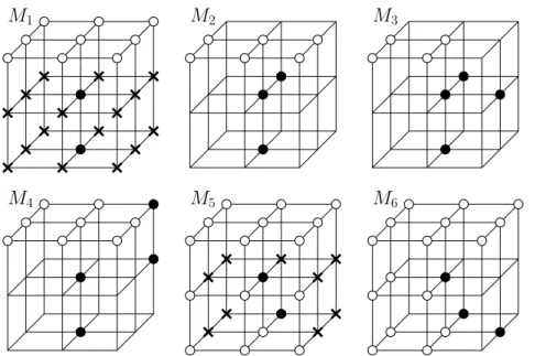
5.4 Masks used for crucial cliques detection. . . 42
5.5 New masks for 2-crucial points detection . . . 45
5.6 New masks for 1-crucial points detection . . . 46
5.7 New masks for 0-crucial points detection . . . 47
5.8 Images used for the benchmark. . . 51
5.9 Computation speed results for ACK3 implemented with different levels of opti-mization. . . 52
5.10 Computation speed results for PKD6 implemented with different levels of opti-mization. . . 52
5.11 Speed gain obtained by different optimizations on ACK3. . . 53
5.12 Speed gain obtained by different optimizations on PKD6. . . 53
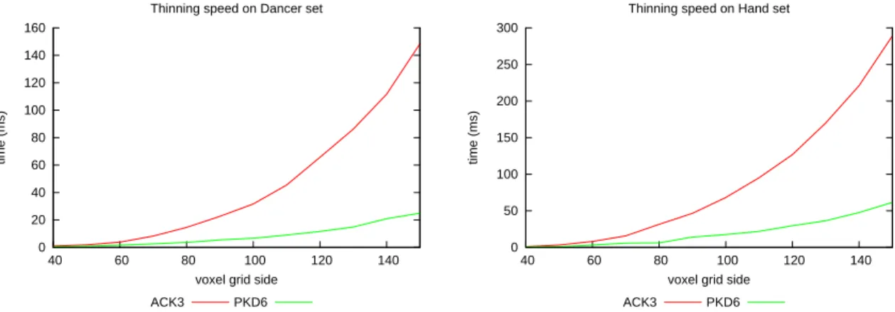
5.13 Thinning speed of fully optimized ACK3 and PKD6 on two data sets. . . 54
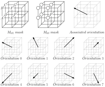
6.1 Masks used in Pal´agyi and Kuba 6-directional thinning . . . 59
6.2 New end points masks . . . 61
6.3 Masks used in our isthmus-based 6-directional thinning . . . 62
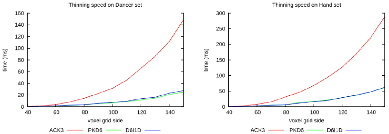
6.4 Thinning speed of fully optimized ACK3, PKD6 and D6I1D on two data sets. . . 63 xiii
6.5 Skeletons resulting of different algorithms for several shapes . . . 64
6.6 Skeletons resulting of different algorithms for several shapes . . . 65
6.7 Examples of homotopic kernels obtained using D6U. . . 66
6.8 Surface skeletons obtained using D6I2D. . . 66
7.1 Example of undirected graph representation . . . 74
7.2 Illustrations of undirected graph properties . . . 75
7.3 Example of directed graph representation . . . 75
7.4 Example of associated undirected graph . . . 76
7.5 Illustrations of directed graph properties . . . 77
7.6 Illustration of isomorphism . . . 77
7.7 Example of labeled graph representation . . . 78
7.8 Example of weighted graph representation . . . 78
7.9 Areas in the shape where we have to find usable spatial positions to represent in the data tree. . . 80
7.10 Classes of skeleton points in both asymmetric and symmetric skeletons . . . 81
7.11 Example of connected components of classes of skeleton points . . . 82
7.12 Example of data tree construction for incomplete model . . . 82
7.13 Examples of spurious branches and ghost limbs . . . 83
7.14 Illustration of useless vertices problem . . . 83
7.15 Illustration of splitted vertices problem. . . 84
8.1 Examples of edit operations for labeled rooted trees. . . 88
8.2 Examples of edit operations for weighted trees. . . 88
8.3 Example of mapping for labeled rooted trees . . . 90
8.4 Example of invalidate mapping for weighted rooted trees . . . 91
8.5 Example of alignment and alignment mapping. . . 93
8.6 Example of constrained mapping . . . 94
8.7 Illustration of the center of three vertices . . . 94
8.8 Example of invalidate constrained mapping . . . 95
8.9 Illustration of less constrained mapping . . . 95
8.10 Example of top down mapping . . . 96
8.11 Example of bottom-up mapping. . . 97
8.12 Hierarchy of mappings.. . . 97
8.13 Example of alignment for weighted trees . . . 100
9.1 Example of merging on directed graph. . . 102
9.2 Examples of merging on undirected graph. . . 102
9.3 Examples of homeomorphism. . . 102
9.4 Example of merging kernel of an undirected graph. . . 103
9.5 Example of merging kernel of a directed graph. . . 103
9.6 Example of homeomorphic alignment. . . 104
9.7 Example of pruned tree . . . 106
9.8 Illustration of possible rooting of unrooted tree . . . 110
9.9 Examples of cut operations . . . 116 9.10 Example of bad homeomorphic alignment matching due to merging on model tree 118 10.1 Example of asymmetric homeomorphic relations on a set of homeomorphic trees. 121
11.1 Illustration of structural noise generation . . . 128
11.2 Illustration of precision measurement . . . 128
11.3 Precision without weight variation . . . 129
11.4 Precision with 10 percent of weight variation . . . 129
11.5 Precision with 50 percent of weight variation . . . 130
11.6 Example where alignment provide better result than homeomorphic alignment. . 131
11.7 Computation speed of different alignments for different sizes of trees. . . 132
11.8 Distributions for a grid sided by 40. . . 133
11.9 Distributions for a grid sided by 80. . . 133
11.10Distributions for a grid sided by 120. . . 134
11.11Average distributions. . . 134
11.12Frequencies of asymmetric homeomorphic alignment of hand rooted model tree with different rooted data trees. . . 135
11.13Frequencies of asymmetric homeomorphic alignment of full human body rooted model tree with different unrooted data trees. . . 136
11.14Average frequencies of asymmetric homeomorphic alignment for different sizes of grid. . . 136
12.1 Detailed pipeline of our method . . . 143
12.2 Example of high limb length variations . . . 143
12.3 Illustration of betweenness problem . . . 144
12.4 Examples of trivial betweenness relations . . . 146
12.5 Illustration of intuitive betweenness relation . . . 147
12.6 Example of non intuitive mathematically correct betweenness relation . . . 149
12.7 Example of more intuitive mathematically correct betweenness relation. . . 150
12.8 Complete pipeline of our method . . . 151
12.9 Full description of two different subjects . . . 151
13.1 Samples of the different used data sets . . . 155
13.2 Speed results for three different data sets . . . 156
13.3 Examples for the different classes of matchings . . . 157
13.4 Study of correlations between AHA distance and matching quality for dancer data set . . . 158
13.5 Study of correlations between AHA distance and matching quality for children data set . . . 159
13.6 Study of correlations between AHA distance and matching quality for hand data set(Rb). . . 160
13.7 Study of correlations between AHA distance and matching quality for hand data set(Ri) . . . 162
13.8 Samples of output poses for different models. . . 163
13.9 Sample of accuracy difference of pose estimation for different grid resolutions . . 164
List of Tables
5.1 Look Up Tables for Crucial Point Detection . . . 48 5.2 Summarize of Optimizations Speed Gain (results expressed as ”average [min, max]”) 53 11.1 Time complexities of the different alignments. . . 127 11.2 Time complexities of the different alignments, taking into account the bounded
maximal degree. . . 132
List of Algorithms
1 Basic Thinning(X, W , D, k) . . . 30
2 Parallel Thinning(X) . . . 31
3 Directional Thinning(X) . . . 33
4 Subfield Based Thinning(X) . . . 34
5 Result Retrieval in Binary Decision Tree . . . 40
6 CK Thinning . . . 43
7 ACK Thinning . . . 44
8 Optimized ACK Thinning. . . 48
9 Optimized CK Thinning . . . 49
10 PKD6 . . . 58
11 D6I1D . . . 60
12 τd . . . 62
13 Data tree construction. . . 81
14 Homeomorphic Alignment Distance for Rooted Trees . . . 109
15 Order of navigation computation algorithm (computeOrder) . . . 112
16 Homeomorphic Alignment Distance for Unrooted Trees . . . 113
17 Homeomorphic Alignment Distance between Rooted and Unrooted Trees . . . 115
18 Asymmetric Homeomorphic Alignment Distance for Rooted Trees . . . 124
Introduction
Global Introduction
“Notre nature est dans le mouvement, le repos entier est la mort.” (“Our nature consists in motion; complete rest is death.”)
Blaise Pascal.
1.1
Background
Motion capture consists in automatic estimation of the pose (i.e. relative position and orientation of each part of the subject), motion and actions of a subject, usually a full human being. It is an highly active research field since more than twenty years, notably due to its industrial applications in computer-animated feature films and Human-Computer Interfaces (HCI). For the latest, some specific properties are required:
• Real-time computation, in order to provide good interaction. • The subject must not need to wear specific equipment (markers).
Usual markerless motion capture systems are composed by a set of cameras, providing the input information of the subject. Numerous markerless methods of motion capture use an a priori model describing the structure and shape of the subject whom motion has to be captured. Such methods are composed of at least two steps: the initialization step, where the initial pose and the parameters of the model are detected, and the tracking step, consisting of finding the current pose in function of the previous ones.
In many of such methods, the initialization step is done manually by the user, forbidding the possibility to be used for HCI purpose, or requires constraining actions or poses of the subject.
1.2
Contribution
In this thesis, we propose an automatic real-time markerless initialization step using a very simple a priori model, described by a tree (called model tree), which can be easily designed in order to use the method for any kind of subject, e.g. full human being, hand, or dog.
Our method uses topological information (the skeleton) extracted from a 3D reconstruction of the subject, obtained by using a multi-camera system. This topological information is then represented by a tree (called data tree), which will be matched with the model, in order to find the position of specific parts, e.g. head, torso, crotch, arms and legs in the case of full human being.
In order to reach our goal, we have done some contributions in different fields of research:
Digital Topology. As our method requires real-time computation, we have worked on opti-mizations of the speed of skeletonization algorithms and on design of new fast and efficient skeletonization schemes.
Graph Theory. The matching between the model tree and the data tree has to take into consideration some specific noises on the data tree, due to its acquisition. We have proposed a definition of matching that is adapted to our needs, and associated computationally efficient algorithms.
Motion Capture. Merging the results of our previous works, we provided an efficient auto-matic real-time markerless initialization step. We also introduced novel intuitive constraint definitions, which can be optionally added to the model definition, in order to improve the robustness of the method.
The structure of this manuscript is in four parts: the first one introduces the background and the backbone of our method, and the three others deal with our contributions and results in the three fields of research enumerated above, respectively.
Motion Capture Overview
Automatic capture and analysis of articulated 3D subjects (e.g. humans, hands or animals) motion is an highly active research area since more than twenty years.
Motion capture presents issues in several kinds of applications:
3D models animation: motion capture is widely used for movies and video games characters animation. Usage of real actors movements to animate virtual avatars is faster, more accurate and realistic than doing it manually.
Human-computer interfaces (HCI): several usages can be done of motion capture in the field of HCIs, including domotic (control of TV or HIFI by hand moves), sign language understanding, or virtual reality system interactions.
Surveillance: motion capture can be used in surveillance field in order to detect suspect be-haviors, e.g. fights or theft, or crowd analysis.
Medical analysis: motion capture can be used for medical purpose, in order to analyze gait problems or high level sportsmen performances.
Of course, all these applications do not require the same properties for motion capture. Ani-mation and medical analysis request a very accurate motion capture and analysis in order to be usable, but it can be done offline (i.e. after the performance of the subject). On the other hand, HCI and surveillance applications need a real-time motion capture, in order to allow an immediate response for some given situations but the accuracy is less essential, and only requires to allow the understanding of the action or the approximate location of the subject parts. There exists numerous different methods to perform motion capture. In the sequel of this chapter, we propose a non exhaustive state of the art on motion capture, focusing on the class of methods used in the thesis, and on their specificities. For exhaustive studies, the reader can refer to [116,117,140].
2.1
Overview of Motion Captures Systems
2.1.1 Acquisition Systems Using Markers
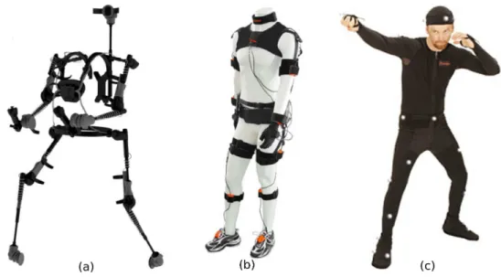
Several acquisition systems estimate motion of a subject by measuring the position and/or the orientation of physical objects (called markers), which are fixed on the subject at specific loca-tions. Acquisition systems with markers are widely proposed as commercial soluloca-tions. Different classes of such system can be defined, in regard of the method used to measure marker positions:
• Mechanical systems (e.g. GypsyTM system, see Figure2.1a) estimate the motion by direct
measurement of articulation angles, via potentiometers fixed on an exoskeleton. The main problem of such systems is the fragility of the skeleton, which can be easily broken.
• Magnetic systems (e.g. MotionStarTM and FastrakTM systems) consist in generating an
electromagnetic field then finding the position and orientation of markers (coils of electric wire) by their perturbation of the field. The main problem of such system is the sensitivity to interferences from metal objects of the environment.
• Inertial systems (e.g. ColibriTM and XsensTM systems, see Figure 2.1b) use markers
com-posed by accelerometers and gyroscopes. These sensors provide motion informations, as speed and rotation of the marker. Then, softwares are used in order to find the pose of the subject from these informations. A very famous inertial motion capture system is the
WiimoteTM. The main problem of such system is the lack of accuracy, in regard of other
methods.
• Optical Systems can be classified in two categories:
– Passive optical systems (e.g. OptiTrackTM, see Figure2.1c, and QualisysTMsystems)
use cameras in order to track markers coated with a retroreflective material reflecting light generated near the cameras lens.
– Active optical systems (e.g. PhaseSpaceTMsystem) use markers powered to emit their
own light (via a LED).
The main problem of such systems is the sensibility to self occlusions: all the markers are not detected by all cameras, some of them being hidden by parts of the body.
These acquisition systems using markers have in common to be very expensive, due to the requested specific hardware.
2.1.2 Marker Free Optical Acquisition Systems
Contrary to other acquisition systems, marker free optical acquisition systems only require cam-eras. We can classify marker free methods in regard of the requested number of cameras:
Figure 2.1: Examples of systems using markers. (a) exoskeleton of GypsyTM
mechanical system. (b) markers of XsensTM
inertial system. (c) markers of OptiTrackTM
passive optical system.
Monocular Methods. Pose estimation from only one video stream is a very complex problem, notably due to self occlusions of subject parts. This kind of method is mainly used for surveillance purpose, crowd study and hand gesture recognition.
Multi-view Methods. During the last twenty years, the increase of computer power has al-lowed the management of multiple synchronized cameras and fast computation of 3D representation of the subject. It led to the development of numerous multi-view methods, freed from the problem of self occlusions. A majority of these methods requires a static background and a prior camera calibration.
According to Menier et al. [111], most of the markerless methods fall into three categories:
• Learning-based methods [1,6,9,58,119,156,163,171,174] store a set of training examples whose poses are known and estimate pose by searching for training images similar to the input images. This category of methods requires larger storage memory space than others. • Model-free methods [27, 36, 42, 43, 48, 104, 105, 161, 176] do not require any a priori
knowledge and automatically recover articulated structures.
• Model-based methods use an a priori model which is tracked using image information.
Moeslund et al. [116,117] defined a general structure of such methods in four steps:
1. Initialization. Ensuring that the system starts motion capture with a correct inter-pretation of the scene: initial subject pose, background images, model parameters are some of the possible informations acquired during this step.
2. Tracking. Using temporal information in order to find the current parameters of the model (e.g. position and orientation of the different parts) from the previous ones. 3. Pose estimation. Estimating the pose of the subject in function of the model
param-eters.
4. Recognition. Recognizing the actions, activities and behaviors of the subject.
Classically, tracking and pose estimation steps are merged in one step. Here, we consider that recognition step is a problem distinct from motion capture.
Since in this thesis, we exclusively deal with markerless multi-view model-based methods, we will focus on the main characteristics of this kind of method.
2.2
A priori Model Definitions
Numerous model definitions have been proposed in the literature. A wide majority of them includes a kinematic structure (also called kinematic skeleton) defined by:
• a set of segments with specified lengths, representing limbs,
• a set of joints linking segments, with specified degrees-of-freedom, representing articula-tions.
Although some methods only require a kinematic structure [35, 111], most of them require to
link it with shape information.
A usual way to provide shape information is the use of geometric primitives, like ellipsoids [31],
truncated elliptical cones [79–81], super-quadric [166,167], or combinations of several kinds [45, 112–115].
Another usual way to provide shape information is to use a surface, which can be generated
from geometric primitives [66, 139] (implicit surface), or an accurate mesh acquired in a prior
step by a specific device [51,76]. Notice that in some cases [3,50], such meshes are used without kinematic skeletons.
In addition to kinematic and shape information, color information can be used, by texturing the
mesh [11], or giving some additional color priors [112] (e.g. noticing that hands and head are
the only parts to have the same color).
Figure 2.2: Examples of model definitions. (a) Kinematic model used by Menier et al. [111]; (b) Super-quadratic representation used by Sundaresan and Chellappa [166]; (c) Ellipsoid rep-resentation used by Horaud et al. [66] and (c’) its associated implicit surface; (d) A surface scan of an actress and (d’) corresponding mesh used by De Aguiar et al. [3]; (e) Textured mesh and
(e’) its underlying skeleton used by Ballan and Cortelazzo [11].
2.2.1 Adaptability of the Models
The adaptability of the method, i.e. the simplicity to modify the method in order to use it for another subject than the one initially targeted, obviously depends on the model definition. We define two levels of adaptability:
• inner-class adaptability is the simplicity to modify the model in order to use it for another subject of the same kind (e.g. two different human beings)
• trans-class adaptability is the simplicity to modify the model in order to use it for a subject of different kind (e.g. from full human body to hand motion capture)
Models using only kinematic structure, geometric primitives and implicit surfaces have a high inner-classes adaptability, model parameters being adjusted during initialization step, contrary to meshes, which have to be rebuild in a prior step, using specific devices and methods.
Concerning the trans-classes adaptability, almost all the methods can be used for any kind of subject, if an adapted model is provided (such methods are called generic). The exception is
subject [112,114,115]. For all the others, the trans-classes adaptability is inversely proportional to the complexity of the model.
2.3
On the Use of Multi Camera Systems
Motion capture methods use information provided by multi-camera systems in many different ways, and can be classified into two categories: methods using 3D reconstruction of the subject and methods performing projection of the model in the images.
2.3.1 Projection in Images
Projection of the model in images can be performed by several methods, in order to use specific information which is easier and faster to extract in 2D than in 3D. Examples of information are:
• silhouette [50] and contours of the subject [45, 79–81], methods searching for a optimal
fitting of the model in each of them.
• connected components of a same color [2], methods using them to facilitate the fitting.
• optical flow of contours [167], specific projected points [11] or shape descriptors [3, 51]
(e.g.SIFT [47]) can be performed in order to track the motion in all the images
indepen-dently, then reconstruct the 3D motion by triangulation.
2.3.2 3D Reconstruction of the Subject
Another approach consists of directly using 3D clues, considering 3D data resulting from multi-view modeling methods.
2.3.2.1 Stereo-Correlation
A famous binocular modeling method is the stereo-correlation, used in some methods [45,139]:
when cameras have a small baseline and are pointing in about the same direction, a part of the surface of the subject is visible in both images. It is thus possible to estimate the depth of this surface part by studying the disparity between corresponding points in the two images.
2.3.2.2 Visual Hulls
The most used multi-view modeling method is the visual hull, introduced by Laurentini [89]:
intuitively, an object lies inside the volume generated by back-projecting its silhouette through the camera center (called silhouette cone). The intersection of the silhouette cones of all the
cameras results in a volume called the visual hull (see Figure 2.3for some illustrations), which
is guaranteed to contain the object. Two kind of visual hulls can be distinguished:
• surface visual hull, used in [111], consists in only representing the surface of the visual
hull by a mesh. Some methods, e.g. [66], use in addition the information from normals to
surface elements.
• volumetric visual hull, used in [114, 115], consists in representing the visual hull volume
by a subset of a voxel grid positioned at the intersection of all images cones: a voxel belongs to the visual hull if and only if the projection of it center in each image belong the corresponding silhouette. The voxels can be colorized [31, 35,76,112, 113] using ray tracing from the cameras, providing additional information. Volumetric visual hull can be
computed in real-time, using GPU [63], or hierarchical carving [31].
Notice that some methods [166] use both visual hull and projection in images.
Figure 2.3: (a) Illustration of silhouette cones, reprinted from Matusick et al. paper [109]. (b) Example of input camera image and associated silhouette. (c) and (d) Illustrations of surface and volumetric visual hulls reconstructions, respectively: object is represented in blue, its silhouettes in green, silhouette cones by dashed lines, and result by bold lines. (e) and (f) surface and volumetric visual hulls of a same object, respectively. Figures (b), (e) and (f) are
2.4
Initialization Step of Model-Based Methods
A wide part of model-based motion capture methods found in the literature focus on the tracking and pose estimation step, and often omit the initialization step.
The initialization step is though essential, as providing the parameters of the model (limb lengths, dimensions of geometric primitives, color information, initial position and orientation of the different parts) which are primordial for an efficient tracking.
Different solutions have been proposed in the literature:
1. manual initialization [111] consists of manually setting the initial values of the model.
2. limb by limb identification [35] consists of asking to the subject to successively move only
each of its limbs, in a specific order, in order to easily identify which part of subject
information (in the case of Cheung et al. [35], a visual hull) is associated to each part of
the model.
3. some methods require a specific initial pose [31,35,76], most often an “X”-pose, where the subject have spread legs and arms. It allows a fast identification of the model parameters, as the limb positions are already approximately set.
4. the initialization can be automatically done, using a hierarchic fitting [112–114]: due to
its unique shape and size, the head is the easiest part to find and is identified first. Then, the torso is located using head position information, and finally limbs are detected using torso position and orientation information.
The method 1 is difficult to use online, for HCI purpose for example. It is even more a shame,
as some methods using it (e.g [111]) are able to perform real-time tracking.
On the other hand, methods 2 and 3 can be used online, but such methods involve some con-straints for the subject, which have to perform special actions in order to be tracked.
Finally, method 4 can be used online and does not require any specific action or pose from the subject, but is not generic: if the subject does not contain a part which is easy to detect, the initialization cannot be performed.
For our best knowledge, no real-time generic initialization step method has been proposed in the literature.
Motivation
As seen in the previous chapter, numerous methods of marker-free 3D motion capture require a manual initialization of the subject pose or a constraining one, e.g. needing a special pose of the subject.
The aim of our work is to provide a pose initialization method (i.e. resulting only in the positions of specific parts of the subject) with several properties. First, our method has to be generic, in the sense it must be adaptable for a large set of subjects (full human body, hands, upper part of the human body, animals...) only by creating a very simple a priori model. Our method has to be real-time, in order to be usable with real-time tracking for online applications. Furthermore, we request our method to be robust, i.e. to work for a large set of subject poses, avoiding constraints for the subject. Finally, we consider that the input of the method is only a volumetric visual hull of the subject.
This chapter is composed of two sections. In the first one, we discuss the definition of the a priori model required by our method. Then, in the second section, we propose a brief overview of the pipeline of our method.
3.1
Model Definition
3.1.1 Constraints of Descriptors
The choice of the descriptors used for our a priori model definition is linked to different obser-vations, according to the nature of the application and to our philosophy.
As we consider only the visual hull in input, we do not use any color information, contained in the camera images. No color prior is used in our method. Furthermore, some models have homogeneous color, e.g. hands, thus such information is not enough generic.
The quality of the 3D shape depends of the number of views for the visual hull reconstruction, and the respective positions of the cameras. In a multi-view system without enough cameras, or not well positioned ones, the visual hull can present important variations of limbs thickness in regard of the subject. Due to this fact, we do not use accurate shape representations, like geometric features.
As we want to create a method that should be usable with any kind of subject, we have to propose a representation allowing to easily describe the subject. We thus avoid the use of shape primitive description and laser scanned models.
Our method has to be able to find the pose of the subject in a maximum number of situations, in order to be able to perform the initialization step as often as possible. By this way, we can use our method even when the subject does not perform a specific action or pose (like it is usually the case), and we can check the tracking at closer intervals, increasing the accuracy.
The weakest constraint we found is that the topology of the shape and its salient geometric features have to be the same as for the model.
3.1.2 Model Description
Taking into consideration all the constraints enumerated in the previous section, we propose an a priori model providing a description of the topology and of the geometric features of the subject, using a tree representation.
The model is built as follows:
• Each vertex represents a characteristic part of the model. For example: – for the full human body: hands, feet, head, torso and crotch.
– for the hand: the arm, the palm (in two parts), the end of the fingers. • Two vertices are linked if the associated parts are adjacent in the model.
• To each edge is associated a weight, corresponding to the approximative distance (for a given distance unit used for all the weights in the graph) between the two linked parts.
Two kinds of models can be considered (see Figure 3.1for examples):
• the complete models, for subjects fully contained in the 3D acquisition space, as in the case of full human body motion capture, for example.
• the incomplete models, which are part of a biggest shape, as in the case of hand pose estimation. In this case, a part of the shape intersects the border of the 3D acquisition space (e.g. the arm, in case of hand motion capture), and we represent this part in the model as an infinite limb, as we do not know it length.
6 4 7 7 7 7 +∞ 4 10 12 12 16 16 // the arm // the palm // the finger root // the thumb // the index // the middle finger // the ring finger // the little finger
Edges: A-P=infinity P-F=4 P-T=6 F-I=7 F-M=7 F-R=7 F-L=7 A P F T I M R L // the head // the torso // the crotch // the first arm // the second arm // the first foot // the second foot
Edges: H-T=4 T-C=10 T-H1=12 T-H2=12 C-F1=16 C-F2=16 H T C A1 A2 F1 F2 A P F T I M R L Vertices: H T C A1 A2 F1 F2 Vertices:
Figure 3.1: Description of two different models. On the Left, the hand model (incomplete model): notice that the edge between the arm and the palm is weighted by “infinity”, as we do
not know its length. On the right, the full human body model (complete model).
Notice that the use of a tree, instead of a graph, for the model description, forbid the represen-tation of models containing holes (represented by a loop in a graph), but allow faster algorithms for the matching with data.
3.2
Initialization Method Overview
Now we have defined the inputs of our method: a visual hull representation of the subject and the a priori model.
Our method consists in extracting a descriptor from the visual hull (called the data descriptor ) which is similar to the one used in the a priori model (called the model descriptor ). The main difference is that the data descriptor has to contain some spatial information, where as that the model descriptor contains informations about the nature of the parts of the model.
Finding a matching between the two descriptors results in finding spatial information for each part of the model and by this way, the pose of the subject.
3.2.1 Extraction of Data Tree
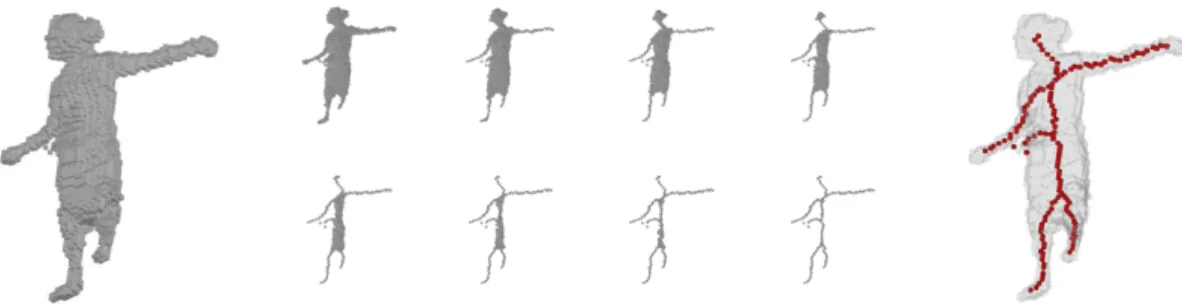
First we have to find a way to extract topological and geometrical information from the visual hull, and to represent it by a tree. We solve this problem in two steps: first, we consider the skeleton of the visual hull. The skeleton is an efficient shape descriptor, representing in a compact form the topology and the main geometric features of a shape. It can be obtained by
iteratively removing voxels without changing the topology (see Figure 3.2for an example).
Figure 3.2: Example of skeletonization process. Left: a visual hull. Middle: different steps of skeletonization process. Right: resulting skeleton (in red).
• Each vertex represents a characteristic point of the skeleton: ending point or intersection point.
• Two vertices are linked if the associated points are adjacent to a same curve in the skeleton. • To each edge is associated a weight, which is the number of voxels in the corresponding
curve.
In the case of incomplete model, we have to consider that a branch ended by a point touching
the border of acquisition space have an infinite length. See Figure 3.3for some examples of data
tree extractions.
More details about data tree extraction are given in Chapter 7.
8 23 22 10 6 12 24 29 +∞ 4 15 16 8 13 20 22 14 4 7
Figure 3.3: Examples of data tree extraction. Left: for a full human body subject. Right: for a hand subject. The black disk represents a point of the skeleton touching the border of the
acquisition space.
3.2.2 Matching Data Tree with Model Tree
Once we have a tree description of the subject, we have to find a way to match it with the model tree. In the literature, numerous methods are proposed to find a matching between two trees. However, in our case we have to take into consideration several kind of noises in the data tree. Furthermore, in the literature, proposed methods are designed for special kind of trees, usually rooted, oriented, and with information on vertices instead of on edges, as in our case.
We have to define a new way to match our data tree with our model tree, corresponding to our constraints.
3.2.3 Pipeline and Main Difficulties of Our Method
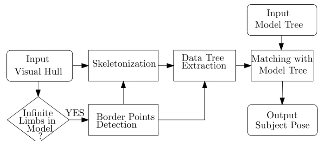
The pipeline of our method is summarized in Figure 3.4.
Visual Hull Skeletonization
Data Tree
Extraction Matching withModel Tree Model Tree
Infinite Border Points
Detection Input Output Input Subject Pose Limbs in Model ? YES
Figure 3.4: Pipeline of our method. Rounded rectangles represent input and output data. Other rectangles represent steps of the method.
We have now defined the different steps of our method, however, two main difficulties remain. First, the skeletonization process has to be both speed efficient and robust to visual hull surface noise. To our best knowledge, no skeletonization algorithm satisfies these two properties. In the second part of this manuscript, we propose some solutions to speed up existent algorithms and a new algorithm providing good skeletons in real time.
The second problem is the matching with the model tree. As explained in Section 3.2.2, no
method found in the literature is adapted to our special case of unrooted edge weighted trees, with special noises on the data tree. In the third part of this manuscript, we propose new kind of matching specially designed for our problem, and efficient algorithms for their computation. Finally, after solving these two main difficulties, we propose in the last part of the manuscript to improve the robustness of the result by addition of intuitive constraints, and we study the results and the speed of our method.
Skeletonization Optimizations
State of the Art of Skeletonization
The skeleton was originally defined by Blum [22] based on a “ grass fire” analogy. Imagine
a shape as a field covered by dry grass; if you set on fire the contour of the field, then the meeting points of the flame fronts would constitute the skeleton of the shape. In the continuous framework, this definition is equivalent to saying that the skeleton is the set of points which are centers of maximal balls (balls included in the object, and not strictly included in any other
such ball) ([32]). Figure4.1shows an example of skeleton in continuous framework.
Figure 4.1: Example of skeleton in continuous framework. The shape (a rectangle) is repre-sented in grey. The skeleton is reprerepre-sented by bold lines. Some maximal balls are reprerepre-sented
by dashed lines, with their center represented by black points.
In 1969, Hilditch gave four properties that a skeleton in a bi-dimensional space should
pos-sess [64]. Adapted to the general case of n-dimensional skeletons, these properties are:
1. a skeleton should be homotopic to the original object,
2. a skeleton should be thin (should have lower dimension than the object), 3. a skeleton should be centered in the original object,
4. skeletonizing a skeleton should not change anything.
In the continuous framework, the set of centers of maximal balls, called the medial axis, satisfies these properties [91,106]. In the discrete framework Zn, the discrete medial axis does not satisfy
two of these properties: it is not always homotopic to the original object, and it is not always
thin (See Figure 4.2for an example).
Figure 4.2: Example of medial axis in discrete framework. The shape is represented in grey. The medial axis is represented by crosses. Some maximal balls are represented by dashed lines,
with their centers represented by bold crosses.
Various methods have now been developed for performing skeletonization of a discrete object.
According to Pal´agyi [129], discrete skeletons can be computed using four types of methods:
Voronoi-based transformations [26, 122], distance-based transformations [23, 172], general-field
methods [5,149] and thinning. In this thesis, we will focus only on thinning methods, as they
are the most studied and well defined.
4.1
Thinning Theory
Thinning consists of iteratively removing points of the object without changing its topology. These points have specific characteristics and are called simple points. In this section, we will first provide usual definitions and notations of digital topology. Using these definitions, we will in a second time describe the characteristics of simple points.
4.1.1 Definitions and Notations
First we have to introduce some fundamental definitions and notations of digital topology.
In digital topology, the framework is the discrete grid Zn. In our case, we will only consider the
cases n = 2 (bi-dimensional) and n = 3 (tri-dimensional). The object is represented by X ⊂ Zn,
and its complementary Zn\ X is denoted by ¯X.
A point p∈ Zn is defined by (p
1, ..., pn), with pi∈ Z.
4.1.1.1 Neighborhood
The notion of neighborhood is central for digital topology. In the 2D case, two neighborhoods
• the 4-neighborhood of p is the set N4(p) ={q ∈ Z2;|q1− p1| + |q2− p2| ≤ 1}.
• the 8-neighborhood of p is the set N8(p) ={q ∈ Z2; max(|q1− p1|, |q2− p2|) ≤ 1}.
p
4
4
4
4
8
p
8
8
8
8
8
8
8
Figure 4.3: Left: 4-neighborhood of p represented by boxes labeled by 4 or p. Right: 8-neighborhood of p represented by boxes labeled by 8 or p.
In 3D case, three neighborhoods (see Figure 4.4) are considered:
• the 6-neighborhood of p is the set N6(p) ={q ∈ Z3;|q1− p1| + |q2− p2| + |q3− p3| ≤ 1}.
• the 26-neighborhood of p is the set N26(p) ={q ∈ Z3; max(|q1−p1|, |q2−p2|, |q3−p3|) ≤ 1}.
• the 18-neighborhood of p is the set N18(p) ={q ∈ N26(p);|q1−p1|+|q2−p2|+|q3−p3| ≤ 2}.
p
p
p
Figure 4.4: From the left to the right: 6-neighborhood, 18-neighborhood and 26-neighborhood of point p, represented by black disks and p.
For a k-neighborhood, we define Nk∗(p) = Nk(p)\ {p}.
4.1.1.2 Connectivity
From the definition of neighborhood we can propose the definition of connectivity.
Let p be an element of X, we define the k-connected component of X containing p, denoted by
Ck(p, X), as the maximal subset of X containing p, such that for all points a∈ Ck(p, X), there
exists a sequence of points ofhp0, ..., pni such:
• p0 = p and pn= a,
• ∀i ∈ {1, ..., n}, pi−1 is in the k-neighborhood of pi.
The set of all k-connected components of X is denoted by Ck(X). We can notice that the union
of all the elements of Ck(X) is equal to X, and the intersection of two different elements of
Ck(X) is always the empty set.
A subset Y of Zn is k-adjacent to a point p∈ Zn if Y ∩ Nk∗(p)6= ∅. The set of all k-connected
components of X which are k-adjacent to a point p is denoted by Ckp(X).
When we consider the k-connectivity of X, it is mandatory to consider a different ¯k-connectivity
for ¯X [82]. In bi-dimensional space, if k = 4, then ¯k = 8, and inversely. In tri-dimensional space,
if k = 6, then ¯k = 26 and inversely. This rule is necessary in order to retrieve some important
topological properties such as the Jordan theorem.
4.1.1.3 Connectivity Numbers
In order to provide local description of simple points and other characteristic points, we have to introduce the notion of connectivity numbers.
In the 2D case, let X ⊆ Z2 and p ∈ Z2. For k ∈ {4, 8} the connectivity number T
k(p, X) is
defined by:
Tk(p, X) =|Ckp(N8∗(p)∩ X)|
In the 3D case, the definition of connectivity numbers lies on the notion of geodesic neighborhood.
Let X ⊆ Z3 and p ∈ Z3. The t-order k-geodesic neighborhood of p in X is the set Nkt(p, X)
recursively defined by:
• N1 k(p, X) = Nk∗(p)∩ X • Nt k(p, X) = S {Nk(q)∩ N26∗ (p)∩ X, q ∈ Nkt−1(p, X)}
The geodesic neighborhoods Gk(p, X) are defined by: G6(p, X) = N62(p, X) and G26(p, X) =
N261 (p, X).
We can now define the connectivity numbers in 3D, for k ∈ {6, 26} as:
Tk(p, X) =|Ck(Gk(p, X))|
4.1.2 Simple points
4.1.2.1 Simple Points in 2D
Intuitively, a point is simple if it can be removed from an object without changing its topology. In the digital topology framework, the topology of an object depends on the chosen connectivity; for this reason, when considering a k-connected object, we will talk about k-simple points. The notion of simple point is central for homotopic thinning in the digital framework: a skeleton is obtained by iteratively removing simple points from an object.
According to [88], in the 60s, 2D simple points were characterized based on connectivity: a point
p is k-simple for an object X if the removal of p does not change the number of k-connected
components of X nor the number of k-connected components of X [25,56]. This definition does
not lead to efficient algorithms : indeed, in order to test if a single point is simple, it requires to scan the whole object in order to enumerate its connected components. Fortunately, local characterization of deletable points in 2D began to appear in the mid 60s [64,147,150,184]. All these works established that, in order to decide whether a point is deletable or not, it is only necessary to look at the configuration of the point’s neighbourhood (no need to count the number of connected components of the whole object). Consequently, in 2D, deciding if a point is simple can be done in constant time.
Proposition 1. Let X ⊂ Z2, and p∈ X. If T
k(x, X) = 1 and T¯k(x, X) = 1, then p is k-simple
for X.
4.1.2.2 Simple Points in 3D
In 3D, the removal of a point may not only change the number of connected components of the
object, but may also change the tunnels of the object (see Figure 4.5 for an example). As in
the 2D case, 3D simple points can be locally characterized [118]. Further work on 3D simple
points have established that only connectivity of X and X is sufficient in order to characterize 3D simple points [15, 19,102,151, 152]. As in 2D, deciding if a point is simple can be done in constant time in 3D. Bertrand and Malandain propose a local definition of simple points using
connectivity numbers T6 and T26:
Proposition 2. [19] Let X ⊆ Z3 and x ∈ X. The point x is k-simple for X iff T
k(x, X) = 1
(a)
(b)
(c)
Figure 4.5: (a) A shape with a tunnel. (b) Deletion of the red point. (c) The shape has no tunnel.
4.1.2.3 Simple Points in Higher Dimensions
Studies of simple points in 4-dimensions have also been achieved, leading once more to a local
characterization of such points [40,85]. Thanks to these works, characterization of simple points
in 4D can be done again in constant time.
4.2
Different Kind of Skeletons
In this section, we will review the different kinds of results which can be expected from a thinning process. The design and the constraints of the thinning algorithm will obviously depend on the desired result.
4.2.1 Ultimate Skeleton
Let X ∈ Znand Y ∈ Znbe two objects. We say that X and Y are homotopic if we can transform
X in Y by iteratively adding and removing simple points. We say that Y is lower homotopic to X if Y can be obtained from X by iteratively removing simple points.
Let X ∈ Zn be an object. A subset Y ⊆ X is an ultimate skeleton of X if:
• Y is lower homotopic to X
• for any point p of Y , p is not simple for Y .
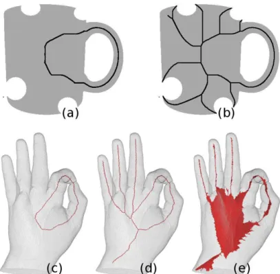
Ultimate skeleton can be used to study the topology of the object, but possibly important
Figure 4.6: Examples of the different kinds of skeleton. Top, 2D skeletons: (a) ultimate skeleton, (b) curvilinear skeleton. Bottom, 3D skeletons: (c) ultimate skeleton, (d) curvilinear
skeleton, (e) surface skeleton.
4.2.2 Curvilinear and Surface Skeletons
Ultimate skeleton, providing only topological information about the shape, is not efficient as a shape descriptor. Some geometric information, like salient parts, have to be kept in the result of the thinning algorithm.
In 2D case, the skeleton has to be 1D or 0D, according to the Hilditch’s criteria. A 1-dimensional skeleton, regardless of the dimension of the original object, is called a curvilinear skeleton (see Fig. 4.6,(b) and (d)).
In the 3D case, always according to the Hilditch’s criteria, the skeleton can be 0D, 1D or 2D. A
2-dimensional skeleton is called a surface skeleton(see Fig. 4.6(e)).
These skeletons provide both topological and geometrical information about the initial shape, which summarize the general form of the object.
The choice of the skeleton dimension depends on the application. We can notice that a surface skeleton corresponds to the analogy of grass fire in 3D, and provides a more accurate descriptor of the initial object. On the other hand, the curvilinear skeleton is smaller than the surface skeleton, and the provided geometric information can be enough for some applications.
In order to obtain curvilinear or surface skeletons instead of ultimate skeleton, several approaches exist: a first one consists of forcing the preservation of medial axis points, another one consists of preserving some locally characterized points, as extremity points or isthmuses.
4.2.2.1 Extremity Points
Extremity points are simple points which have to be kept in the skeleton in order to preserve elongated geometric features.
In the case of curvilinear skeletons, the considered points are those which end a curve, and are called curve extremities. These points can be locally described:
• Let X ⊆ Zn, p∈ X, p is a k-curve extremity iff |N∗
k ∩ X| = 1.
In the case of surface skeletons, the considered points are those that can be found on “surface borders”. To our knowledge, there is no consensus on the definition of surface border in digital topology.
In addition to this problem, the other one is the sensitivity of this approach to small variations. It results in skeletons containing more branches than needed to represent the geometric features. These additional uninteresting branches are called spurious branches.
4.2.2.2 Isthmus
In order to solve the problems mentioned above, another strategy has been recently developed by
Bertrand and Couprie [18]. Instead of searching for simple points which have to be kept in order
to preserve geometric features, we can search for non simple points having certain topological characteristics. These points are called isthmuses.
For a curvilinear skeleton, the considered isthmuses are the 1D− isthmuses (see Figure4.7for
some examples). In the case of surface skeleton, the considered isthmuses are the 2D−isthmuses.
The main advantage in regard of surface borders is that 2D-isthmus are locally well defined.
In 2D, let X ⊆ Z2, p∈ X, p is 1D-isthmus iff T
k(p, X)≥ 2.
In 3D, let X ⊆ Z3, p ∈ X, p is 1D-isthmus iff T
k(p, X) ≥ 2. The point p is 2D-isthmus iff
Figure 4.7: Examples of 1D isthmuses.
4.2.2.3 Symmetric versus Asymmetric Skeletons
Another distinction has to be done between the different kind of skeletons: symmetric and asymmetric ones. This notion of symmetry is due to interpretation in the digital framework of two of the four properties of the skeleton proposed by Blum: the centering and the thinness properties.
Assume that we have an efficient thinning process which thins an object layer by layer. It can lead to sets of simple points which cannot be all removed together without breaking the topology. We have then two choices: we can keep all these points or we can arbitrarily remove a subset of them in order to have a thin skeleton.
The first choice leads to a symmetric skeleton: it is well centered but it is not thin. A symmetric skeleton is closer to the medial axis as it preserves more maximal ball centers.
The second choice leads to an asymmetric skeleton: it is thin but not well centered, due to arbitrary choices.
4.3
Thinning Algorithms
Homotopic thinning in the digital framework consists of removing simple points from an ob-ject, until either no more simple point can be found (resulting in an ultimate skeleton), or a satisfactory subset of voxels has been reached (resulting in a surface or curvilinear skeleton). Two main strategies are possible for removing simple points: sequential removal and parallel removal.
4.3.1 Sequential algorithms
Sequential removal of simple points can be achieved by detecting simple points in an object, and removing them one after the other, until no more simple point can be found. After removing a simple point, the new set of simple points of the object must be computed. Such basic strategy does not guarantee the result, which is an ultimate skeleton, to be centered in the original object.